
Submitted:
03 August 2025
Posted:
04 August 2025
You are already at the latest version
Abstract
Volatility modelling is a key feature of financial risk management, portfolio optimisation, and forecasting, particularly for market indices such as the JSE Top40 Index, which serves as a benchmark for the South African stock market. This study investigates volatility modelling of the JSE Top40 Index log-returns from 2011 to 2025 using a hybrid approach that integrates statistical and machine learning techniques through a two-step approach. The ARMA(3,2) model was chosen as the optimal mean model, using the \texttt{auto.arima()} function from the \texttt{forecast} \texttt{package} in \textts{R} (version 4.4.0). Several alternative variants of GARCH models, including sGARCH(1,1), GJR-GARCH(1,1), and EGARCH(1,1), were fitted under various conditional error distributions (i.e., STD, SSTD, GED, SGED, and GHD). The choice of the model was based on AIC, BIC, HQIC, and LL evaluation criteria, and ARMA(3,2)-EGARCH(1,1) was the best model according to the lowest evaluation criteria. Residual diagnostic results indicated that the model adequately captured autocorrelation, conditional heteroskedasticity, and asymmetry in JSE Top40 log-returns. Volatility persistence was also detected, confirming the persistence attributes of financial volatility. Thereafter, the ARMA(3,2)-EGARCH(1,1) model was coupled with XGBoost using standardised residuals extracted from ARMA(3,2)-EGARCH(1,1) as lagged features. The data was split into training (60ARMA(3,2), EGARCH(1,1), Forecasting, Hybrid model, JSE Top40 Index, Machine Learning, Risk Management, Time Series, Volatility Modelling, XGBoost.%), testing (20%), and calibration (20%) sets. Based on the lowest values of forecast accuracy measures (i.e., MASE, RMSE, MAE, MAPE, and sMAPE), along with prediction intervals and their evaluation metrics (i.e., PICP, PINAW, PIWA, and PINAD), the hybrid model captured residual nonlinearities left by the standalone ARMA(3,2)-EGARCH(1,1) and demonstrated improved forecasting accuracy. This highlights the robustness and suitability of the hybrid ARMA(3,2)-EGARCH(1,1)-XGBoost model for financial risk management in emerging markets and signifies the strengths of integrating statistical and machine learning methods in financial time series modelling.
Keywords:
ARMA(3
; 2)
; EGARCH(1
; 1)
; forecasting
; hybrid model
; JSE Top40 Index
; machine learning
; risk management
; time series
; volatility modelling
; XGBoost
1. Introduction
1.1. Overview
The global stock market, known for its complexity and constant evolution, has consistently drawn the attention of both investors and researchers alike. Several factors influence the movement of stock prices, such as macroeconomic conditions, key economic indicators, market sentiment, company performance, and various other elements. Volatility, described by [1] as the size of price variations in a security or market index over time. Predicting and modelling volatility is crucial for investors, financial analysts, and regulators, as it plays a key role in risk management and asset pricing. The Johannesburg Stock Exchange (JSE) Top40 Index is a 40-share index representing the top 40 largest companies listed on JSE. It consists of multinational corporations with substantial operations in South Africa and across the world. The index is also used to create exchange-traded funds (ETFs) and derivatives, providing investors with broad exposure to the South African equities market.
The modelling of volatility has evolved significantly, beginning with the foundational ARCH model by [3] and its extension to the GARCH model by [2]. While GARCH models are capable of capturing time-varying volatility, they often struggle with nonlinear and asymmetric market behaviours. Financial data frequently exhibit stylised facts such as volatility clustering, leverage effects, and heavy tails, which may not be fully captured by traditional GARCH models.
Besides traditional econometric models, hybrid models combining machine learning (ML) with statistical techniques have shown promise for volatility forecasting. A case in point is the GARCH-XGBoost hybrid model, in which GARCH captures linear time structures and XGBoost, a very powerful tree-based ML model [4], captures nonlinearities. Studies such as ref. [5] demonstrated that these hybrid models substantially improve forecast accuracy in volatile markets. However, their application in the South African context, particularly with the JSE Top40 Index, has been limited. In light of these developments, the primary aim of this study is to develop a modelling framework for assessing the volatility of the JSE Top40 Index using a hybrid GARCH-XGBoost approach, with the intention of improving risk forecasting accuracy. Specifically, the study seeks to explore the volatility behaviour of the JSE Top40 Index, construct and evaluate a hybrid GARCH-XGBoost model, and provide recommendations on risk management and financial decision-making in the South African market using the results of volatility modelling.
This research investigates the application of the hybrid GARCH-XGBoost model in simulating the volatility of the JSE Top40 Index based on historical daily closing prices for 2011–2025. Compared to the standalone traditional GARCH method, this research develops a knowledge base in volatility modelling and forecasting in emerging markets. This entails the incorporation of flexible statistical techniques and machine learning into a more robust and improved volatility estimation system. The study will likely aid financial analysts, investors, and policymakers by improving risk forecasting tools and informing strategic decision-making, with potential implications for other emerging markets.
1.2. Literature Review
1.2.1. Traditional Volatility Models
ARCH and GARCH Models
The foundation of volatility modelling in financial markets was laid by [3] with the establishment of the Autoregressive Conditional Heteroskedasticity (ARCH) model, which allowed the variance of asset returns to vary over time in response to past errors. This was later extended by [2] through the Generalised Autoregressive Conditional Heteroskedasticity (GARCH) model, which incorporated both lagged conditional variances and past squared innovations. GARCH models are now recognised as cornerstone of volatility forecasting, effectively capturing volatility clustering (a phenomenon where periods of high volatility tend to be followed by high volatility and low volatility by low volatility). Nonetheless, despite their widespread application and empirical progress, GARCH-type models encounter notable limitations, particularly in accounting for nonlinear dependencies and asymmetrical effects of positive and negative shocks on volatility.
Extensions of GARCH Models
To tackle the inherent flaws of the basic GARCH model, a number of extensions have been proposed. Ref. [12] proposed the Exponential GARCH (EGARCH) model, and ref. [13] proposed the Glosten, Jagannathan and Runkle GARCH (GJR-GARCH) model that accommodates asymmetric shock effects on volatility. These models perform very well in financial markets, as negative shocks have more impact on volatility than the same magnitude positive shocks, which is known as the leverage effect. Although they are more sophisticated, these models have the disadvantage of being parametric and do not always reproduce the rich dynamics of real financial time series data.
1.2.2. Machine Learning in Volatility Forecasting
eXtreme Gradient Boosting Algorithm
In ML algorithms, XGBoost (eXtreme Gradient Boosting) has become very popular as one of the best techniques for forecasting time series data due to its effectiveness and prediction performance. XGBoost is a gradient boosting technique that creates an ensemble of decision trees by iteratively fitting the model to the residuals produced by the preceding trees. XGBoost has shown strong ability in financial applications such as volatility forecasting, largely due to its ability to detect complex, nonlinear relationships and interactions among variables. Several studies have found that XGBoost often outperforms traditional econometric models in this area [14,15], owing to its strength in capturing the underlying patterns and dependencies present in financial data.
1.2.3. Hybrid Modelling Approaches
GARCH-XGBoost Hybrid Approach
A promising hybrid approach entails combining the GARCH model with XGBoost. In this approach, the GARCH model is first used to model the linear volatility dynamics, and the residuals from the GARCH model are then used as input features for the XGBoost algorithm. This hybrid GARCH-XGBoost model has been shown to improve forecasting accuracy, especially in capturing complex patterns that are not adequately addressed by traditional GARCH models alone. The ability of this approach to blend statistical theory with data-driven learning methods makes it a powerful tool for modelling volatility, particularly for indices like the JSE Top40.
1.2.4. Empirical Studies on the JSE and Other Similar Stock Markets
Empirical Studies on GARCH Models
Ref. [16] carried out an analysis of stylised facts and volatility patterns of the FTSE/JSE Top40 index. The study employed both parametric and non-parametric approaches, using a Markov-switching GJR-GARCH(1,1) model to assess conditional volatility. The research findings demonstrated the presence of volatility clustering, monthly seasonal effects, and significant autocorrelation in logarithmic returns. The FTSE/JSE Top40 index exhibited a 98.8% probability of long memory, while its volatility showed a 99.6% probability of long memory.
Ref. [17] analysed the impact of listing and trading futures contracts on the underlying stock index volatility behaviour, concentrating on the FTSE/JSE Top40 index. The study employed a modified GARCH model, incorporating a dummy variable to capture the non-constant variance of residuals. By dividing the sample period into pre- and post-futures eras, the research found that the introduction of futures contracts increased the volatility persistence of index returns.
Ref. [18] investigated the structure of return volatility on the JSE Securities Exchange of South Africa by employing ARCH-type models. The standard GARCH(1,1) model provided the best description of return dynamics compared to more complex augmentations. Additionally, the BDS test indicated that the model significantly, though not fully, accounts for nonlinearities in the series.
Using daily stock market returns from the JSE, ref. [19] examined the relative performance of the asymmetric normal mixture GARCH (NM-GARCH) model. The empirical results showed that the NM-GARCH model performed better than any other competing models, suggesting that incorporating a variety of errors improves volatility models’ ability to predict financial time series dynamics.
Ref. [20] aimed to forecast volatility in the JSE and the AEX using GARCH models. The study analysed data from 2010 to 2021 and found that market volatility is relatively high on both exchanges. The research demonstrated that volatility persists in both markets, with return movements following similar trajectories.
Empirical studies on hybrid GARCH and Machine Learning approaches
Ref. [4] proposed a hybrid model combining ARIMA, GARCH, and XGBoost to improve the accuracy of stock opening price predictions. The model modifies ARIMA residuals utilising GARCH and XGBoost, leveraging their complementary strengths. Empirical results on Hong Kong stock data indicated that this hybrid approach outperforms traditional single models and other hybrid models in terms of accuracy and robustness.
Ref. [24] analysed hybrid modelling for stock market forecasting by combining ARIMA-GARCH models with machine learning models such as support vector machines (SVM) and long-short-term memory (LSTM) networks. Applied to NASDAQ, DAX, NSE, and BIST index data, the hybrid models significantly enhanced prediction accuracy over single models, effectively detecting linear and nonlinear trends in finance time series.
Ref. [25] investigated the forecasting of high-dimensional asset return covariance matrices through the integration of GARCH processes and neural networks. The proposed model includes forecasting volatilities through hybrid neural networks while correlations take a standard econometric approach. Under a minimum variance portfolio framework, the hybrid model outperforms equally weighted portfolios and its econometric counterparts with univariate GARCHs.
1.2.5. Summary and research gap
The literature review illustrates that despite the popularity of classical GARCH models and their extensions in forecasting volatility, they are not capable of capturing complex nonlinearities and asymmetries in the financial time series data. ML algorithms, most notably XGBoost, have been shown to be helpful in addressing these limitations. Yet, minimal research has applied these advanced models to the JSE Top40 Index, particularly with hybrid approaches. This study aims to bridge this gap by the application of the hybrid GARCH-XGBoost model to model the volatility of the JSE Top40 Index. By combining statistical modelling and machine learning, this study will offer a better and more robust approach to volatility forecasting in South African financial markets.
1.3. Contribution and Research Highlights
1.3.1. Contribution of the Study
This study contributes to the growing body of literature on financial time series forecasting by proposing a novel hybrid volatility modelling approach that integrates traditional statistical models (ARMA(3,2)-EGARCH(1,1)) and machine learning (XGBoost) through a two-step approach. The main contribution is the prospective ability of this hybrid model to enhance forecast performance and detect complex nonlinear patterns that may not be captured by standalone models, particularly when applied to emerging markets such as the JSE Top40 Index. The study emphasises the need to integrate traditional econometric and machine learning models to facilitate effective financial risk management and decision-making.
1.3.2. Highlights of the Study
Research highlights:
- Proposed a hybrid ARMA(3,2)-EGARCH(1,1)-XGBoost model for improved volatility forecasting.
- Used a two-step modelling approach, combining statistical and machine learning techniques.
- Demonstrated that the hybrid model effectively captures nonlinear residual structures left by standalone models.
- Achieved superior forecasting performance based on MASE, RMSE, MAE, MAPE, and sMAPE.
- Evaluated prediction intervals using PICP, PINAW, PIWA, and PINAD, with improved interval accuracy and reliability.
- Highlighted the potential of hybrid models in financial risk forecasting in emerging markets.
- Emphasised the importance of model fusion in achieving both accuracy and robustness in time series volatility forecasting.
The remainder of this research is outlined as follows: Section 2 discusses the methodological framework, Section 3 presents empirical results and analysis, and Section 4 concludes the study with key findings and recommendations.
2. Methodology
2.1. Data Collection and Preprocessing
2.1.1. Data Collection
The study is going to use daily closing prices of the JSE Top40 Index for a specific time period from 2011 to 2025. The data, which is freely available, can be accessed on https://za.investing.com/indices/ftse-jse-top-40-historical-data. The data is collected over a five-day trading week.
2.1.2. Data Preprocessing
The dataset will be checked for possible anomalies, such as missing values and outliers, which could affect the accuracy of the volatility models. For outlier detection, visual methods such as boxplots and histograms will be used to identify extreme values. These visualisations permit for an intuitive understanding of the data distribution and help to detect potential outliers. If outliers are detected, appropriate actions such as removal or transformation will be considered. For handling missing data, the deletion method will be applied, where rows containing missing values will be removed if the missing data is not substantial.
Furthermore, log returns will be calculated from the raw daily closing price data to transform the data into a format that is more appropriate for volatility modelling. Log returns are preferred as they allow for the assumption of stationarity in the time series data. The log return for each time period will be computed using the formula:
where is the log return at time t, is the closing price at time t and is the closing price of the previous day. These preprocessing steps, including outlier detection, handling missing values, and log return transformation, will ensure that the data is clean, reliable, and ready for modelling.
2.1.3. Stationarity Check
The stationarity of the data will be checked through time series plots. If the data appears non-stationary, differencing methods will be applied to achieve stationarity. Then, the Augmented Dickey-Fuller (ADF) and Kwiatkowski-Phillips-Schmidt (KPSS) tests will be carried out to confirm whether the data is stationary. After differencing and testing, a visual check of the transformed data will be done once more to ensure stationarity before moving forward with the modelling process.
2.1.4. Autocorrelation and Heteroskedasticity Detection
Financial time series typically exhibit autocorrelation and patterns of conditional heteroskedasticity that violate classical ordinary least squares (OLS) assumptions and lead to inefficient or biased estimates. Autocorrelation describes the linear dependence of lagged values of a time series, whereas heteroskedasticity refers to non-time-constant error variance. It is essential in financial modelling, particularly in forecasting and estimating volatility, to detect such characteristics. In this subsection, we present two visual plots and two statistical tests: ACF and PACF plots for autocorrelation, the Box-Ljung test of autocorrelation, and Engle’s ARCH LM (Lagrange Multiplier) test of heteroskedasticity.
2.1.5. Normality Test
The Jarque-Bera (JB) test is a statistical test used to determine if a given sample of data follows a normal distribution. Unlike other tests, the JB test focuses on the skewness (asymmetry) and kurtosis (tailedness) of the data. In the case of a normal distribution, the skewness should be 0, and the kurtosis should be 3. Since financial time series data often exhibit non-normal characteristics, such as skewed returns or fat tails, the JB test is particularly useful in analysing such data.
2.2. GARCH Models
2.2.1. Standard GARCH Model
When modelling the dynamic changes in volatility, the ARCH model requires estimating a large number of parameters, which makes predictions more complex and variable. In contrast, the GARCH model incorporates additional conditional variance terms , reducing the complexity of parameter estimation. This gives the model better long-memory properties and a more flexible time-lag structure. Since GARCH is commonly used in empirical research, this study focuses on it, where equation 2 represents the mean equation and equation 3 defines the variance equation.
where and denotes the log-returns of the JSE Top40 Index at time t and conditional mean of the log-returns, respectively. is modelled using the ARMA( model defined as:
is the error term (log-returns shocks or innovations) defined as:
where with mean zero and variance 1.
2.2.2. Glosten, Jagannathan and Runkle GARCH Model
The Glosten, Jagannathan and Runkle GARCH (GJR-GARCH) model is a type of asymmetric GARCH model that introduces dummy variables to differentiate the impact of positive and negative shocks on volatility. This helps capture the varying effects of market fluctuations more accurately. The most commonly used version is GRJ-GARCH(1,1), which builds on the standard GARCH (sGARCH(1,1)) model by incorporating a dummy variable. The variance equation of the GJR-GARCH model is given by equation 4 as shown below.
where is an indicator function that accounts for asymmetry.
2.2.3. Exponential GARCH Model
The Exponential GARCH (EGARCH)) model is another asymmetric volatility model, but unlike traditional GARCH models, it models the logarithm of variance instead of the variance itself. This approach ensures that volatility remains positive without requiring parameter restrictions. If the coefficient is positive, it suggests that fluctuations in the time series persist over time, a phenomenon known as volatility clustering. The variance equation for the EGARCH model is presented in equation 5.
2.3. eXtreme Gradient Boosting Model
The eXtreme Gradient Boosting (XGBoost) model is a powerful ML algorithm based on extreme gradient boosting. It follows a boosted tree approach, where each tree refines its predictions by minimising the difference between the estimated and actual values [11]. Mathematically, XGBoost can be represented as a summation, as illustrated in Equation 6.
where is the predicted value for the -observation, K is the total number of trees, represents the prediction from the -tree and is the the space of regression trees.
The objective function in XGBoost consists of two main components, i.e the loss function, which measures the difference between the predicted and actual values, and a regularisation term that controls model complexity. It is given by:
where is the regularisation term, is the loss function measuring the difference between the actual and predicted values, T is the umber of leaves in the tree, are the leaf weights, and and are regularisation parameters that control model complexity.
At each -boosting step, a new tree is added to the model as shown in equation 9:
where is the final prediction after -boosting iterations.
The objective function is approximated using 2nd-order Taylor expansion shown in equation 10:
where and represents gradient and Hessian, respectively. The main objective is to optimise in each step.
The optimal weight of each leaf j is given by:
where is the set of data points in leaf j.
The gain function helps to identify the best tree split and is given by the equation 12:
where and are the left and right child nodes, respectively. The split with the highest gain is considered.
2.4. GARCH-XGBoost Hybrid Model
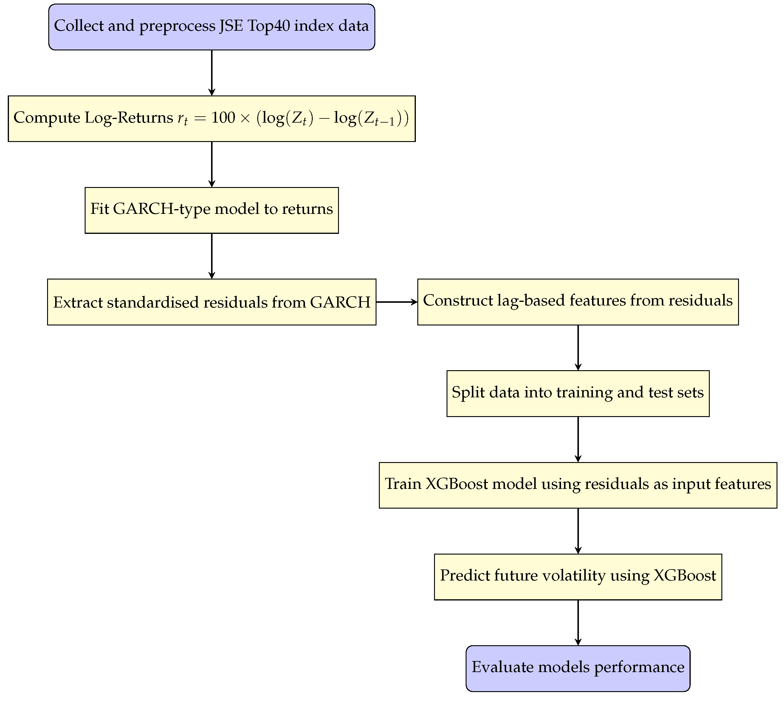
Figure 1.
GARCH-XGBoost diagram workflow.
2.5. Conditional Distributions and Parameter Estimation
In volatility modelling, particularly with GARCH models, the selection of an appropriate conditional distribution is essential. This distribution governs the behaviour of the residuals or returns given the past information and impacts the model’s flexibility in capturing various features such as fat tails, skewness, and asymmetry. These are the most commonly used conditional distributions that can be employed with these models: Student-t Distribution (STD), Skewed Student-t Distribution (SSTD), Generalised Error Distribution (GED), Skewed Generalised Error Distribution (SGED), and Generalised Hyperbolic Distribution (GHD). The model’s parameters were estimated using Maximum Likelihood Estimation (MLE).
2.6. Evaluation Metrics
To assess the performance of models, we use evaluation metrics such as Log-likelihood (), Akaike Information Criterion (), Bayesian Information Criterion (), and Hannan-Quinn Information Criterion (). The R software package is used to compute the value of , , and . The formulas for , , and are given by the following equations 13:
where denotes the maximised log-likelihood, denotes the estimated variance of the model’s errors, k represents the number of estimated parameters in the model, and n is the sample size. The model with the lowest value of , and is considered.
2.7. Forecast Accuracy Measures
To evaluate how well the prediction model performs, this study employs several accuracy metrics, including the Mean Absolute Square Error (MASE), Mean Absolute Error (MAE), Root Mean Square Error (RMSE), Mean Absolute Percentage Error (MAPE), and Symmetric Mean Absolute Percentage Error (sMAPE).
2.8. Prediction Interval Evaluation Metrics
Prediction interval evaluation metrics are used to assess the quality of prediction intervals (PIs) generated by a model. These metrics consider two main aspects: how often the true values fall within the intervals (called coverage) and how wide the intervals are (sharpness). Below are commonly used metrics:
2.8.1. Prediction Interval Coverage Probability
Prediction Interval Coverage Probability (PICP) measures the proportion of true values that fall within the predicted intervals. Its mathematical equation is given by:
where, n is the number of observations, is the true value, , represent lower and upper bounds of the prediction interval, and denotes the indicator function (I if condition is true, 0 otherwise).
2.8.2. Prediction Interval Normalised Average Width
Prediction Interval Normalised Average Width (PINAW) measures the average width of prediction intervals, normalised by the range of the target variable. It’s equation is given as:
where, denotes the range of true values.
2.8.3. Prediction Interval Normalised Average Deviation
Prediction Interval Normalised Average Deviation (PINAD) quantifies the average deviation between the interval midpoint and the true value. Its equation is given by:
2.8.4. Prediction Interval Coverage Average -Normalised Width
Prediction Interval Coverage Average-Normalised Width (PICAW) measures the average width of prediction intervals that successfully captured the true values. Its equation is given as:
These metrics provide a comprehensive understanding of how reliable and informative the prediction intervals are in capturing the true variability of the target variable.
3. Empirical Results and Discussion
3.1. Exploratory Data Analysis (EDA)
3.1.1. Graphical and Statistical Diagnostics of the JSE Top40 Index and it’s Log-Returns
Figure 2 shows the time series plot of the JSE Top40 closing price index from the year 2011 to 2025. The plot is mainly upward-sloping, indicating a general increase in the index over the observed period. The time series plot indicates visible spikes, suggesting some level of volatility, particularly with a drastic drop in early 2020 that is likely to have been brought about by the global impact of the COVID-19 pandemic. Following this downfall, the index exhibits a strong recovery and continues rising. The oscillations vary in magnitude with time, capturing different levels of volatility, a common feature of financial time series and conducive to the application of advanced volatility models such as GARCH-XGBoost and GAS. There also does not appear to be any clear-cut seasonal trend in the data, which indicates the absence of periodic recurring effects. Non-stationarity of both the mean and variance of the series indicates the need to transform it into log-returns to facilitate more robust statistical analysis and forecasting.
Figure 3 provides a preliminary exploration of the JSE Top40 daily log returns through various graphical techniques. Panel (a) illustrates the time series plot of the log returns, which were obtained by first differencing the log-transformed price series to induce mean stationarity, which is a necessary condition for most time series modelling techniques. The resulting series has a zero mean and exhibits volatility clustering, where periods of high volatility tend to follow each other, implying conditional heteroskedasticity. Panel (b), the histogram superimposed with a normal density curve, reveals that the distribution is leptokurtic and slightly negatively skewed and thus implies the presence of heavy tails and asymmetry in the behaviour of the returns. This is also confirmed by panel (c), the Q–Q plot, with significant deviation from the diagonal line in both tails, confirming non-normality as well as excess kurtosis. Panel (d), the boxplot, shows that values cluster around the median with a few outlier observations outside the whiskers, also confirming outliers and the fat-tailedness of the distribution. Overall, these findings suggest the presence of non-normality, volatility clustering and extreme returns.
Figure 4 shows the missing value plot for each variable of the JSE Top40 index. The plot indicates that there are no missing observations in any of the variable columns. Overall, this suggests that the JSE Top40 index dataset contains no missing values.
Figure 5 shows the ACF and PACF plots of the JSE Top40 Index daily log returns, providing information about the presence of autocorrelation in the log return series. The ACF plot illustrates a series of significant spikes, particularly in the early few lags, beyond the 95% confidence levels, to signify that the log returns are autocorrelated. Similarly, the PACF plot also shows high peaks at various lags, again reflecting a sign of autocorrelation present in the log return series. These visual inspections are also confirmed by the results in Table 1 that show the Box-Ljung Q test statistics for various lag lengths. In all the lags which have been reported (), test statistics are greater than their corresponding critical values, and the p-values are substantially below the level of 5%, and the null hypothesis of no autocorrelation is therefore rejected. Overall, these findings establish statistically significant autocorrelation in JSE Top40 log returns.
Figure 6 displays the ACF and PACF plots of the squared log returns of the JSE Top40 Index, which are used for identifying second-order dependence (autocorrelation in the variance). Both plots exhibit significant and slowly decaying autocorrelations at multiple lags, especially in the ACF plot, indicating that there is long-lasting autocorrelation in the squared log returns. This is the traditional sign of conditional heteroskedasticity, with the implication that the variance of the log returns is time-varying. Table 2 provides formal proof of this finding through Engle’s ARCH LM test at various lag lengths. At all lags (), the test statistics are far greater than the corresponding critical values, with p-values smaller than , leading to a decisive rejection of the null hypothesis of no ARCH effects. These results confirm the presence of conditional heteroskedasticity in the squared log returns.
Table 3 summarises the results of stationarity and normality tests applied to the log returns. Both ADF and KPSS tests indicate that the log return series is stationary. However, the JB test strongly rejects the null hypothesis of normality (because ), implying that the log returns are not normally distributed.
Table 4 shows the descriptive statistics of the log-returns of the JSE Top40 index, which reveal significant characteristics about the nature of the log-return distribution. The mean is approximately , indicating a slight upward trend in the average daily log-returns over the sample period. The distribution is moderately dispersed with a standard deviation (SD) of , signifying a high level of volatility. The minimum (Min) and maximum (Max) values of and , respectively, suggest the presence of extreme log-return values, possibly due to market shocks or outliers. The negative skewness (Skew) coefficient of implies that the log-return series is slightly skewed to the left, meaning that extreme negative log-returns are more dominant than extreme positive ones. Moreover, the kurtosis (Kurt) value of exceeds the benchmark value of 3 for a normal distribution, exhibiting a leptokurtic distribution characterised by heavy tails and a higher probability of extreme log-returns. The deviation from normality in the distribution is further evidenced by the JB test in Table 3, which confirms that the log-return series does not follow a normal distribution. These stylised features regarding the negative skew and excess kurtosis are typical of financial time series data and suggest that models accounting for asymmetry and fat tails may be more appropriate for modelling the volatility of JSE Top40 log-returns.
3.2. Selection of the ARMA(p,q) Mean Model
The mean model for the log-returns was selected by using the auto.arima() function from the forecast package in R (version 4.4.0). The function used ARMA models with Autoregressive (AR) and Moving Average (MA) of a maximum order of 10. Based on information criteria, the most suitable model was found to be ARMA(3,2) with zero mean, which implies that the mean dynamics of the series are best described by an AR(3) and MA(2) model.
3.2.1. ARMA(3,2) Mean Model Diagnostics
Figure 7 is a plot of the residual values after fitting the ARMA(3,2) mean model to the log returns of the JSE Top40 Index. The residuals move randomly around zero, indicating that the model has effectively removed the linear dependence trend in the mean. However, the graph shows periods of high and persistent volatility, particularly during and around 2020, which is most likely a reflection of the shocks that hit the markets during the COVID-19 pandemic. These clusters of large residuals point towards volatility clustering, which implies the residuals are not homoskedastic. This graphical evidence suggests the likely presence of conditional heteroskedasticity in the residuals.
Figure 8 shows the ACF plot of the residuals of the fitted ARMA(3,2) model for the JSE Top40 log returns. While most of the autocorrelation coefficients lie within the 95% confidence bounds, there are statistically significant spikes for some of the lags, which means that not all the autocorrelation was captured in the model. This is confirmed by the Box-Ljung test results shown in Table 5, where the null hypothesis of no autocorrelation is rejected at all lags considered (lags 10 to 30), with p-values consistently below the 5% significance level. These results indicate the presence of remaining autocorrelation in the residuals, implying that the ARMA(3,2) model does not adequately account for all linear dependencies in the return series. Furthermore, the JB test strongly rejects the null hypothesis of normality (p-value ), indicating that the residuals are not normally distributed.
Figure 9 presents a graphical evaluation of the distributional characteristics of the residuals of the ARMA(3,2) model. The histogram (left panel) has a peak close to zero, as one would expect for residuals, but the distribution is leptokurtic (more peaked and heavier-tailed than a normal distribution), indicating non-normality. This is also supported by the Q-Q plot (right panel), in which the points deviate substantially from the 45-degree reference line, especially in the tails. These deviations indicate that the residuals are not normally distributed. This finding is in line with the foregoing JB test result. Fat tails in residuals suggest that the residuals exhibit excess kurtosis, as is common in financial time series, and suggest the potential need for conditional error distributions with heavier tails.
Figure 10 presents the time series plot of the squared residuals of the ARMA(3,2) model for an assessment of the variance’s behaviour over time. Most of the squared residuals are of low magnitude, while the plot contains several bursts of high volatility with a sharply peaked curve at around 2020 that is presumably driven by the COVID-19 pandemic-related financial market crisis. This clustering of large squared residuals is a clear indication of volatility clustering, a stylised fact of financial return series, and points to the presence of conditional heteroskedasticity. The visual evidence from this plot suggests that the variance is not constant over time.
Figure 11 presents the ACF plot of the squared standardised residuals from the ARMA(3,2) model fitted to the JSE Top40 log returns. The plot shows high autocorrelation at a range of lags, and particularly at small orders, with decreases that are comparatively slow as the lag increases. This persistent autocorrelation structure of the squared standardised residuals is very strong and indicates that there is time-varying volatility, i.e., residual variance is time-varying and depends on prior squared values. These findings are statistically confirmed by the results of Engle’s ARCH LM test in Table 6, which reports extremely large test statistics and p-values less than at all considered lags. This leads to a decisive rejection of the null hypothesis of no ARCH effects, indicating the presence of conditional heteroskedasticity in the residuals. Furthermore, Table 7 displays the results of the Box-Ljung test on the squared standardised residuals, with all p-values also being less than , which suggests the presence of conditional heteroskedasticity; that is, the variance of the residuals is serially correlated and changes over time.
3.3. Fitting of ARMA(3,2)-GARCH-type Models
Table 8 provides a comparison of ARMA(3,2)–GARCH-type models fitted under different conditional error distributions: STD, SSTD, GED, SGED, and GHD. The evaluation criteria used are the AIC, BIC, HQIC, and LL. Among all specifications, the ARMA(3,2)-EGARCH(1,1) model under the SSTD exhibits the lowest values for AIC, BIC, and HQIC and the highest LL value. These results suggest that ARMA(3,2)-EGARCH(1,1) with SSTD is the optimal model and provides the best in-sample fit compared to the sGARCH and GJR-GARCH variants under the same distributional error assumptions.
3.3.1. ARMA(3,2)-EGARCH(1,1) Model Diagnostics
Figure 12 displays the ACF plot of the standardised residuals obtained from the ARMA(3,2)-EGARCH(1,1) model. Most autocorrelation coefficients lie within the 95% confidence bounds, with only a few marginally exceeding the limits. This visual evidence indicates that the model has captured the linear dependence structure adequately, as little to no residual autocorrelation remains. This is also supported by the Box-Ljung test of the standardised residuals presented in Table 9. p = 0.309 at lag 1, which is well above the 5% level of significance, and consequently, there is no statistically significant autocorrelation at lag 1. Although lag 14 has p = 0.00087, reflecting residual autocorrelation, the value of p for lag 24 is 0.069, which is only marginally more than the 5% level. Overall, these results confirm that the ARMA(3,2)-EGARCH(1,1) model has indeed eliminated much of the autocorrelation from the residuals, with the residuals that are left being nearly white noise.
Figure 13 shows the ACF plot of the squared standardised residuals of the ARMA(3,2)-EGARCH(1,1) model. There is little significant autocorrelation evident, as most of the spikes are inside the 95% confidence limits, and a couple of small lags reach the boundary. This visual outcome suggests that the conditional heteroskedasticity has been adequately captured by the ARMA(3,2)-EGARCH(1,1) model, leaving little to no remaining structure in the squared standardised residuals. This observation is reinforced by the results of Engle’s ARCH LM test shown in Table 10, where all p-values at lags 3, 5, and 7 are substantially greater than 0.05. Hence, we fail to reject the null hypothesis of no ARCH effects, confirming the absence of remaining conditional heteroskedasticity in the squared standardised residuals. Similarly, Table 11 presents the Box-Ljung test statistics on the squared standardised residuals, which also yield non-significant p-values across all reported lags. This validates the finding that the model has eliminated any remaining conditional heteroskedasticity in the squared standardised residuals. Overall, these results show that the ARMA(3,2)-EGARCH(1,1) model is a good fit for modelling both the average and the ups and downs of the JSE Top40 log returns.
The top panel in Figure 14 shows that the fitted model’s standardised residuals closely follow the fitted SSTD with fatter tails than the normal density. The lower Q-Q plot confirms this by showing that most points are along the 45-degree line, suggesting a good fit, although the slight deviation of the tails suggests some residual non-normality. Overall, the residuals exhibit a distribution with the assumed SSTD.
The News Impact Curve in Figure 15 shows that negative shocks have a greater effect on future volatility than positive shocks of the same magnitude, indicating strong asymmetry. This confirms that the fitted ARMA(3,2)-EGARCH(1,1) model captures the leverage effect present in the data.
The findings in Table 12: Sign Bias Test reveal that the individual terms of sign bias (negative or positive sign) are not statistically significant since their respective p-values are above 0.05. However, the joint effect has a p-value greater than the 5% threshold, providing evidence for asymmetry. These results also align with Figure 15: News Impact Curve, where it is clear that the negative shocks have more influence on volatility than positive shocks.
The mean parameter and the constant term in the variance equation shown in Table 13 are statistically insignificant, as indicated by their p-values greater than , suggesting they do not have a meaningful impact on the model. However, the parameters and are highly significant with p-values , implying that past shocks and past volatility significantly influence current volatility. The model exhibits strong persistence in volatility, as shown by the high value of , indicating that volatility clusters persist over time. Moreover, the positive and significant leverage term suggests evidence of asymmetry, meaning that negative shocks tend to increase volatility more than positive shocks of the same magnitude. This is also demonstrated by the News Impact Curve shown in Figure 15.
3.4. Fitting the hybrid ARMA(3,2)-EGARCH(1,1)-XGBoost Model (Two-Step Approach)
In this section, a two-step approach modelling framework was employed to enhance the forecasting performance and quantify uncertainty in the standardised residual time series. The approach began with fitting an ARMA(3,2)-EGARCH(1,1) model to the daily log returns of the JSE Top40 Index. The autocorrelation linear structure, conditional heteroskedasticity and asymmetry were captured by the ARMA(3,2)-EGARCH(1,1). The rugarch package from R (version 4.4.0) estimated the model under an SSTD for innovations to accommodate both skewness and heaviness in tails. Once the optimal ARMA(3,2)-EGARCH(1,1) model was fitted, the standardised residuals were extracted for further analysis. In the second step, the standardised residuals were modelled using the XGBoost algorithm. This ML method was selected due to its high flexibility in capturing nonlinear patterns and interactions that traditional time series models might overlook. To prepare standardised residuals for XGBoost, a set of lag features (lags 1 to 15) and rolling window statistics (means and standard deviations over window sizes 2, 3, 5, 10, and 20) were generated using data.table and zoo packages in R (version 4.4.0). These features were designed to reflect temporal dependencies and local volatility structure in the standardised residuals.
The prepared data was also split into three sets: 60% for model training, 20% for calibration (for the construction of prediction intervals), and 20% for out-of-sample testing. The XGBoost model was trained on the squared error loss function with a five-fold cross-validation to determine the optimal number of boosting rounds. Hyperparameters were a 0.05 learning rate, an optimal depth of 4, and a subsample ratio of 0.8 to prevent overfitting. Predictions were made on the test and calibration sets after training.To measure how uncertain the forecast is, we used the differences between what we predicted and what actually happened in the calibration set to create 90% prediction intervals. Specifically, the 95th and 5th percentiles of the obtained residuals were used to add to the test set point predictions in order to find the lower and upper bounds of the prediction interval, respectively. For this purpose, the algorithm mimics the conformal prediction principles, wherein the prediction intervals are obtained from the residual distribution over a calibration set, with finite-sample coverage guarantees without strong assumptions on the residual’s distribution. The 90% prediction intervals were complemented by the inclusion of 95% and 99% prediction intervals constructed from the 97.5th/2.5th and 99.5th/0.5th percentiles of calibration residuals. This approach provided a useful way of constructing data-driven nonparametric intervals capturing model uncertainty without strong distributional assumptions. Overall, the two-step approach allowed the power of classical time series modelling (via ARMA(3,2)-EGARCH(1,1)) to be merged with the potential of ML (via XGBoost) to produce accurate point forecasts as well as useful prediction intervals for the standardised residual series.
3.4.1. Forecast Performance Evaluation of Residual-Adjusted Forecasts from hybrid ARMA(3,2)-EGARCH(1,1)-XGBoost Model
Table 14 presents the first ten forecast results obtained from the hybrid model. Each row shows the actual standardised residual and the corresponding point prediction from the model. The table demonstrates that the forecast values are generally close to the actual standardised residuals, indicating that the model performs well in approximating future values. This supports the model’s accuracy in point forecasting and highlights its potential effectiveness in capturing the underlying dynamics of the residuals.
Table 15 shows the forecast accuracy measures of the hybrid ARMA(3,2)-EGARCH(1,1)-XGBoost model fitted using a two-step approach. The hybrid ARMA(3,2)-EGARCH(1,1)-XGBoost model was validated using some measures of the accuracy of forecasts on the test sample of the standardised residuals. MASE is 0.0534 and RMSE is 0.1386, indicating a reasonably low value of the error in the prediction of the model. MAE is 0.0595, suggesting that, on average, the predictions of the model are about 0.06 units away from the actual standardised residuals. MAPE is 27.93%, and sMAPE is 16.41%. These values show moderate relative accuracy of the forecast, and sMAPE is a more accurate and symmetric performance measure of percentage errors that is suited for standardised residuals in which values can be positive as well as negative.
Figure 16 displays the forecast performance of the hybrid ARMA(3,2)-EGARCH(1,1)-XGBoost model on the test set of standardised residuals, along with its corresponding prediction intervals. The actual standardised residuals are plotted in black, while the red line represents the point forecasts generated by the XGBoost component. The shaded region between the dotted green lines is the lower and upper bounds of the empirical prediction intervals constructed based on the calibration residuals. From the Figure 16, there is clear evidence that the hybrid model was tracking the dynamics of the residual series well. The modelled series follows the rise and fall of the actual standardised residuals, including at the points of sharp peaks and troughs. The presence of several extreme spikes, particularly between indices and at index 600, were generally well-bound within the range of the interval, indicating the model’s ability to respond to abrupt volatility.
Furthermore, the vast majority of actual values lie within the prediction intervals, visually supporting the previously reported empirical coverage rate, which exceeds the nominal level. This suggests that the constructed intervals are not only reliable but slightly conservative (an often preferred trait in financial forecasting), where underestimation of uncertainty can have costly implications. Additionally, the temporal average width is fairly consistent with the reported average width of , demonstrating reliable quantification of uncertainty without inflated spread. Altogether, the plot attests to the numerical performance measures and confirms that the hybrid model is precise in point forecasting as well as data-efficient in deriving forecast uncertainty from prediction intervals.
Figure 17 shows that the hybrid model’s prediction intervals effectively capture the uncertainties in forecasts, with of the actual standardised residuals falling within the interval. This indicates slightly conservative, yet reliable, prediction intervals. The average interval width of reflects a reasonable balance between precision and coverage, confirming the model’s strong calibration and forecasting performance.
Figure 18 provides a demonstration of the robustness of the hybrid model’s prediction interval with an empirical coverage rate of . This indicates that nearly all actual standardised residuals fall inside the interval, a remarkable quantification of uncertainty. The average interval width of , while wider than for lower levels, is to be expected and acceptable for so high a confidence level. This wider band enhances the reliability of coverage and makes the model particularly well-suited for risk-attentive forecasting scenarios.
The results of the prediction interval test in Table 16 indicate that the coverage probabilities (PICP) of the 90%, 95%, and 99% intervals are 94.0000%, 97.1429%, and 99.2857%, respectively. These results suggest that the prediction intervals are well-calibrated since they closely estimate or slightly exceed their nominal confidence levels. The normalised average interval widths (PINAD) for the 90%, 95%, and 99% intervals are 0.7939%, 0.7984%, and 0.8130%, respectively, reflecting growing interval width with increased confidence levels. Moreover, both the average interval widths (PINAW) and their scaled values (PICAW) increase with higher confidence levels due to the inherent trade-off between interval sharpness and coverage. Generally, the results indicate that the model is able to produce reliable and informative prediction intervals across all confidence levels.
The time-varying forecast errors plot in Figure 19 indicates the difference between actual and predicted standardised residuals over time. Most errors are around zero, suggesting consistent and unbiased forecasts. There are a few large spikes representing occasional larger forecast deviations, but they are infrequent and not systematic. This reaffirms the model’s ability to generate stable forecasts with occasional outliers, possibly due to unexpected volatility shocks.
4. Discussion and Conclusions
4.1. Discussion
The results of this study validate the performance of the hybrid ARMA(3,2)-EGARCH(1,1)-XGBoost model in volatility forecasting performance improvement in the case of the JSE Top40 Index. Initial mean structure selection using the auto.arima() function identified ARMA(3,2) as the optimal mean model. Subsequent GARCH-type model estimation under varying conditional error distributions identified the ARMA(3,2)-EGARCH(1,1) model under SSTD as the optimal model, as indicated by its lower AIC, BIC, HQIC, and LL values. The EGARCH part picked up significant volatility characteristics such as autocorrelation, asymmetry (leverage effects), and persistence. This was confirmed by residual diagnostics, showing no autocorrelation and heteroskedasticity, thereby confirming the model adequacy. Yet, single statistical models leave residual nonlinearities unaccounted for. To counter this, the hybrid model employed XGBoost to forecast the EGARCH model’s standardised residuals. In a two-step approach, the data were assigned to training (60%), test (20%), and calibration (20%) sets. The model’s performance on the test set showed satisfactory point forecasting accuracy: RMSE = 0.1386, MAE = 0.0595, MASE = 0.0534, and sMAPE = 16.41%, indicating low absolute error and relatively high forecasting efficiency. Table 14 showed that hybrid model point predictions were closely precise relative to actual standardised residuals. Furthermore, Table 15 and subsequent figures confirmed the strong predictive power and credibility of the model. The hybrid model effectively reflected spikes and dips in volatility even in cases of abrupt market changes. Interestingly, prediction intervals for different confidence levels (90%, 95%, 99%) exhibited empirical coverage rates greater than nominal rates, reflecting well-calibrated but conservative intervals, better for financial forecasting use to avoid risk underestimation. The average width of the prediction intervals (i.e., 0.2623 for 90%, 0.4115 for 95%, and 1.3625 for 99%) revealed a good balance between precision and uncertainty. The PICP rates of 94.00%, 97.14%, and 99.29% also supported this. This outcome shows the ability of the model to produce reliable volatility forecasts while maintaining interval prediction points. The hybrid model’s time-varying forecast error analysis showed that most of the residuals were near zero, with occasional large departures occurring. This is indicative of the model generating normally unbiased forecasts with excellent stability and elasticity to volatility shocks. Compared to the standalone ARMA(3,2)-EGARCH(1,1), the hybrid model clearly isolated residual nonlinear patterns in the standardised residuals, enhancing forecasting precision and measurement of risk.
4.2. Conclusions
This research successfully demonstrated the efficacy of combining classical econometric models with advanced machine learning methods to further volatility modelling of the JSE Top40 Index. The ARMA(3,2)-EGARCH(1,1) model with the SSTD distribution was determined to be the best option among competing GARCH-type models, well capturing essential features such as volatility clustering, asymmetry, and persistence of the log returns. The residuals from this model, used for training an XGBoost model, made it possible for the hybrid ARMA(3,2)-EGARCH(1,1)-XGBoost framework to enhance volatility forecasting while considering nonlinear trends and interactions. These results show the potential of hybrid models in financial applications, particularly in markets with high uncertainty, dominance, and complexity of dynamics. Future studies may include expanding the consideration of exogenous macroeconomic variables and deep learning methods to further improve predictive power.
Author Contributions
Conceptualization, I.M., T.R. and C.S.; methodology, I.M.; software, I.M.; validation, I.M., T.R. and C.S.; formal analysis, I.M.; investigation, I.M., T.R. and C.S.; data curation, I.M.; writing—original draft preparation, I.M.; writing—review and editing, I.M., T.R. and C.S.; visualization, I.M.; supervision, T.R. and C.S.; project administration, T.R. and C.S.; funding acquisition, I.M. All authors have read and agreed to the published version of the manuscript.
Funding
This research was funded by the 2025-2026 NRF MSc Postgraduate Scholarship: REF NO: PMDS240701235994
Institutional Review Board Statement
Not applicable.
Informed Consent Statement
Not applicable.
Data Availability Statement
The data were obtained from the Wall Street Journal Markets website https://za.investing.com/indices/ftse-jse-top-40-historical-data (accessed on 25 April 2025).
Acknowledgments
The support of the 2025-2026 NRF MSc Postgraduate Scholarship towards this research is hereby acknowledged. Opinions expressed and conclusions arrived at are those of the authors and are not necessarily to be attributed to the NRF. In addition, the authors thank the anonymous reviewers for their helpful comments on this paper.
Conflicts of Interest
The authors declare no conflicts of interest. The funders had no role in the study’s design, in the collection, analyses, or interpretation of data, in the writing of the manuscript, or in the decision to publish the results.
Abbreviations
The following abbreviations are used in this manuscript:
| ACF | Autocorrelation Function |
| ADF | Augmented Dickey-Fuller |
| AIC | Akaike Information Criterion |
| ARMA | Autoregressive Moving Average |
| BIC | Bayesian Information Criterion |
| EDA | Exploratory Data Analysis |
| EGARCH | Exponential Generalised Autoregressive Conditional Heteroskedasticity |
| GARCH | Generalised Autoregressive Conditional Heteroskedasticity |
| GED | Generalised Error Distribution |
| GJR-GARCH | Glosten-Jagannathan-Runkle Generalised Autoregressive Conditional Heteroskedasticity |
| HQIC | Hannan–Quinn Information Criterion |
| JSE | Johannesburg Stock Exchange |
| JSE Top40 Index | Johannesburg Stock Exchange Top 40 Index |
| KPSS | Kwiatkowski–Phillips–Schmidt–Shin |
| LL | Log-Likelihood |
| MAE | Mean Absolute Error |
| MAPE | Mean Absolute Percentage Error |
| MASE | Mean Absolute Scaled Error |
| MLE | Maximum Likelihood Estimation |
| ML | Machine Learning |
| PACF | Partial Autocorrelation Function |
| PICP | Prediction Interval Coverage Probability |
| PINAD | Prediction Interval Normalised Average Deviation |
| PINAW | Prediction Interval Normalised Average Width |
| PICAW | Prediction Interval Coverage Average -Normalised Average |
| Q-Q | Quantile–Quantile |
| RMSE | Root Mean Square Error |
| sGARCH | Standard Generalised Autoregressive Conditional Heteroskedasticity |
| SGED | Skewed Generalised Error Distribution |
| SSTD | Skewed Student-t Distribution |
| TD | t-Distribution |
| XGBoost | Extreme Gradient Boosting |
| sMAPE | Symmetric Mean Absolute Percentage Error |
References
- Tsay, R.S. Analysis of Financial Time Series, Third ed.; John Wiley & Sons, 2010. [Google Scholar] [CrossRef]
- Bollerslev, T. Generalized Autoregressive Conditional Heteroskedasticity. Journal of Econometrics 1986, 31, 307–327. [Google Scholar] [CrossRef]
- Engle, R.F. Autoregressive Conditional Heteroscedasticity with Estimates of the Variance of United Kingdom Inflation. Econometrica: Journal of the Econometric Society 1982, 50, 987–1007. [Google Scholar] [CrossRef]
- Wang, J.; Zhang, J.; Cai, Y.; others. A Novel Residual Correction Approach Based on a Hybrid GARCH and XGBoost Model. Academic Journal of Computing & Information Science 2024, 7, 127–134. [Google Scholar] [CrossRef]
- Kristjanpoller, W.; Fadic, A.; Minutolo, M.C. Volatility Forecast Using Hybrid Neural Network Models. Expert Systems with Applications 2014, 41, 2437–2442. [Google Scholar] [CrossRef]
- Harvey, A.C. Dynamic Models for Volatility and Heavy Tails: With Applications to Financial and Economic Time Series; Cambridge University Press: New York, USA, 2013; pp. 1–261. [Google Scholar] [CrossRef]
- Junior, P.O.; Alagidede, I. Risks in Emerging Markets Equities: Time-Varying Versus Spatial Risk Analysis. Physica A: Statistical Mechanics and its Applications 2020, 542, 123474. [Google Scholar] [CrossRef]
- Alanya-Beltran, W. Modelling Stock Returns Volatility with Dynamic Conditional Score Models and Random Shifts. Finance Research Letters 2022, 45, 102121. [Google Scholar] [CrossRef]
- Opschoor, A.; Janus, P.; Lucas, A.; Van Dijk, D. New HEAVY Models for Fat-Tailed Realized Covariances and Returns. Journal of Business & Economic Statistics 2018, 36, 643–657. [Google Scholar] [CrossRef]
- Ardia, D.; Boudt, K.; Catania, L. Generalized Autoregressive Score Models in R: The GAS Package. Journal of Statistical Software 2019, 88, 1–28. [Google Scholar] [CrossRef]
- Ribeiro, M. T.; Singh, S.; Guestrin, C. "Why Should I Trust You?" Explaining the Predictions of Any Classifier. Proceedings of the 22nd ACM SIGKDD International Conference on Knowledge Discovery and Data Mining (KDD’16), 2016; 1615–1624. [Google Scholar] [CrossRef]
- Nelson, D.B. Conditional Heteroskedasticity in Asset Returns: A New Approach. Econometrica: Journal of the Econometric Society 1991, 59, 347–370. [Google Scholar] [CrossRef]
- Glosten, L.R.; Jagannathan, R.; Runkle, D.E. On the Relation between the Expected Value and the Volatility of the Nominal Excess Return on Stocks. The Journal of Finance 1993, 48, 1779–1801. [Google Scholar] [CrossRef]
- Wang, Y.; Guo, Y. Forecasting Method of Stock Market Volatility in Time Series Data Based on Mixed Model of ARIMA and XGBoost. China Communications 2020, 17, 205–221. [Google Scholar] [CrossRef]
- Ding, S.; Cui, T.; Zhang, Y. Futures Volatility Forecasting Based on Big Data Analytics with Incorporating an Order Imbalance Effect. International Review of Financial Analysis 2022, 83, 102255. [Google Scholar] [CrossRef]
- Makatjane, K.; Moroke, N. Examining Stylized Facts and Trends of FTSE/JSE TOP40: A Parametric and Non-Parametric Approach. Data Science in Finance and Economics 2022, 2, 294–320. [Google Scholar] [CrossRef]
- Magweva, M.R.; Munyimi, M.M.; Mbudaya, M.J. Futures Trading and the Underlying Stock Volatility: A Case of the FTSE/JSE TOP 40. International Journal of Finance 2021, 6, 1–16. [Google Scholar] [CrossRef]
- Mangani, R. Modelling Return Volatility on the JSE Securities Exchange of South Africa. African Finance Journal 2008, 10, 55–71. [Google Scholar]
- Cifter, A. Volatility Forecasting with Asymmetric Normal Mixture Garch Model: Evidence from South Africa. Journal for Economic Forecasting 2012, 0, 127–142. [Google Scholar]
- Cheteni, P.; Matsongoni, H.; Umejesi, I. Forecasting JSE and AEX Volatility with GARCH Models. African Journal of Business and Economic Research 2023, 18, 461. [Google Scholar] [CrossRef]
- Blasques, F.; Koopman, S.J.; Lucas, A. Stationarity and Ergodicity of Univariate Generalized Autoregressive Score Processes. Electron. J. Statist 2014, 8, 1–31. [Google Scholar] [CrossRef]
- Babatunde, O.; Folorunso, S.; Saliu, F. Comparative Forecasting Performance of GARCH and GAS Models in the Stock Price Traded on Nigerian Stock Exchange. International Journal of Mathematical Modelling & Computations 2021, 11, 1–15. [Google Scholar]
- Yaya, O.S.; Bada, A.S.; Atoi, V.N. Volatility in the Nigerian Stock Market: Empirical Application of Beta-t-GARCH Variants. CBN Journal of Applied Statistics 2016, 7, 27–48. [Google Scholar]
- Bulut, C.; Hudaverdi, B. Hybrid Approaches in Financial Time Series Forecasting: A Stock Market Application. EKOIST Journal of Econometrics and Statistics 2022, 37, 53–68. [Google Scholar] [CrossRef]
- Boulet, L. Forecasting High-Dimensional Covariance Matrices of Asset Returns with Hybrid Garch-Lstms. arXiv 2021. [Google Scholar] [CrossRef]
Figure 2.
Time series plot of the JSE Top40 Price Index.
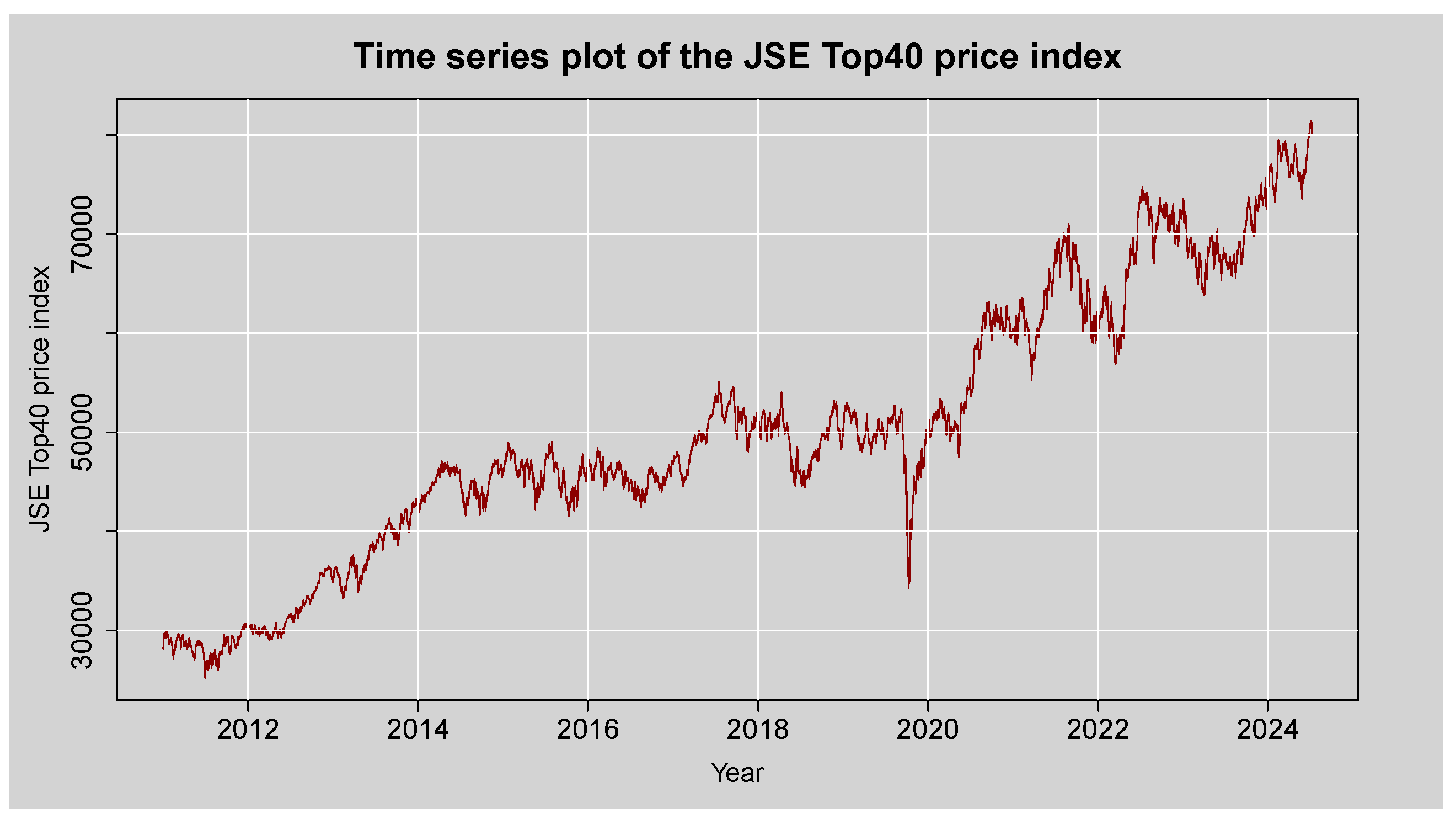
Figure 3.
(a) Log-returns for JSE Top40 stock index, (b) histogram with density curve plot of daily log-returns, (c) normal Q–Q plot of daily log-returns, and (d) boxplot of the JSE Top40 log-returns.
Figure 3.
(a) Log-returns for JSE Top40 stock index, (b) histogram with density curve plot of daily log-returns, (c) normal Q–Q plot of daily log-returns, and (d) boxplot of the JSE Top40 log-returns.
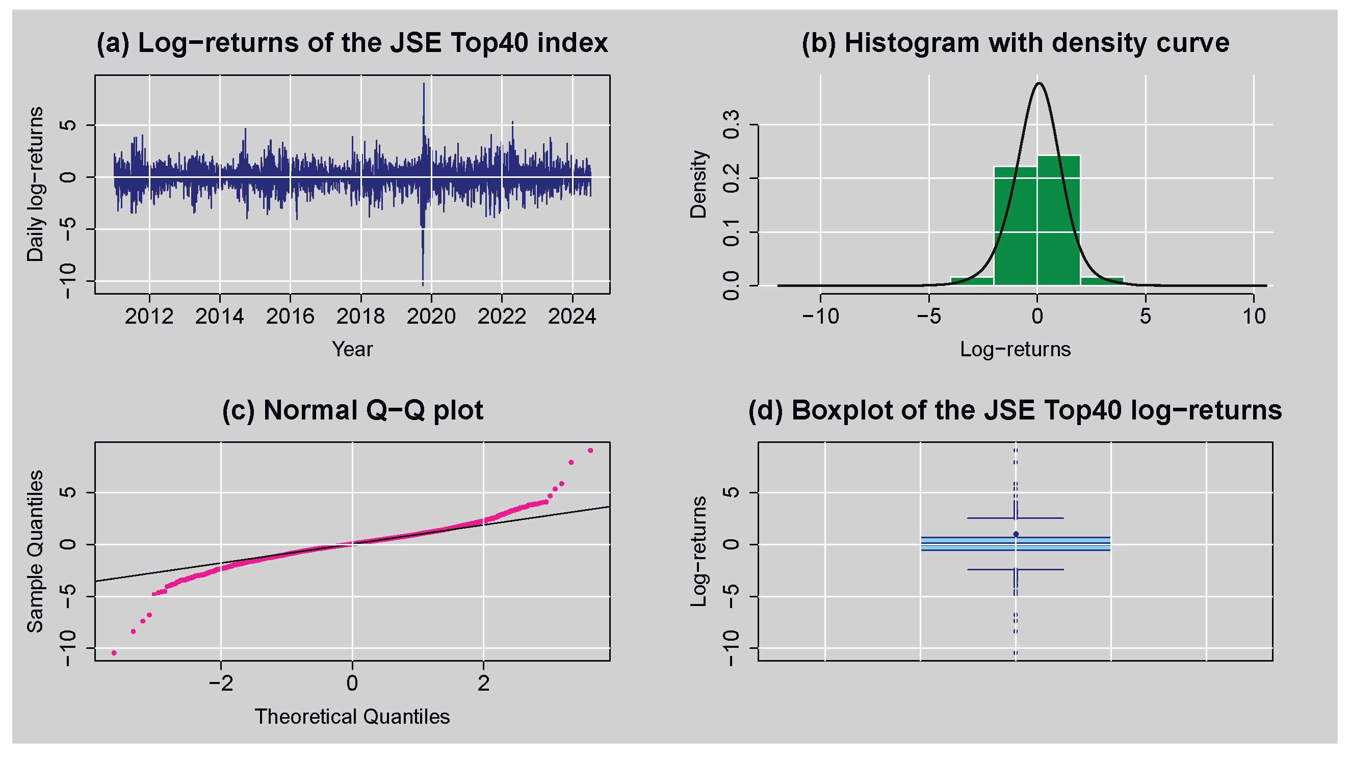
Figure 4.
Missing value plot of each variable of the JSE Top40 index.
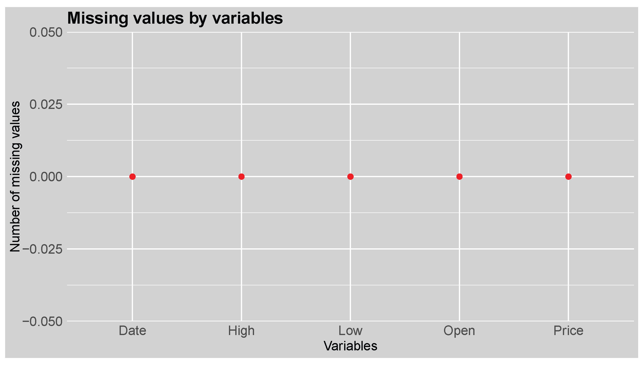
Figure 5.
ACF and PACF plots of the standardised JSE Top40 log-returns.
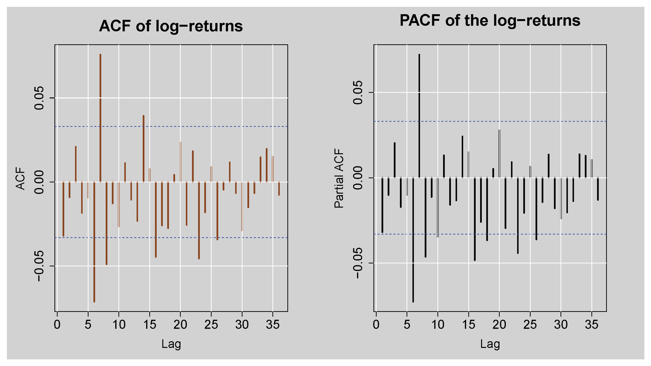
Figure 6.
ACF and PACF plots of the squared standardised JSE Top40 log-returns.
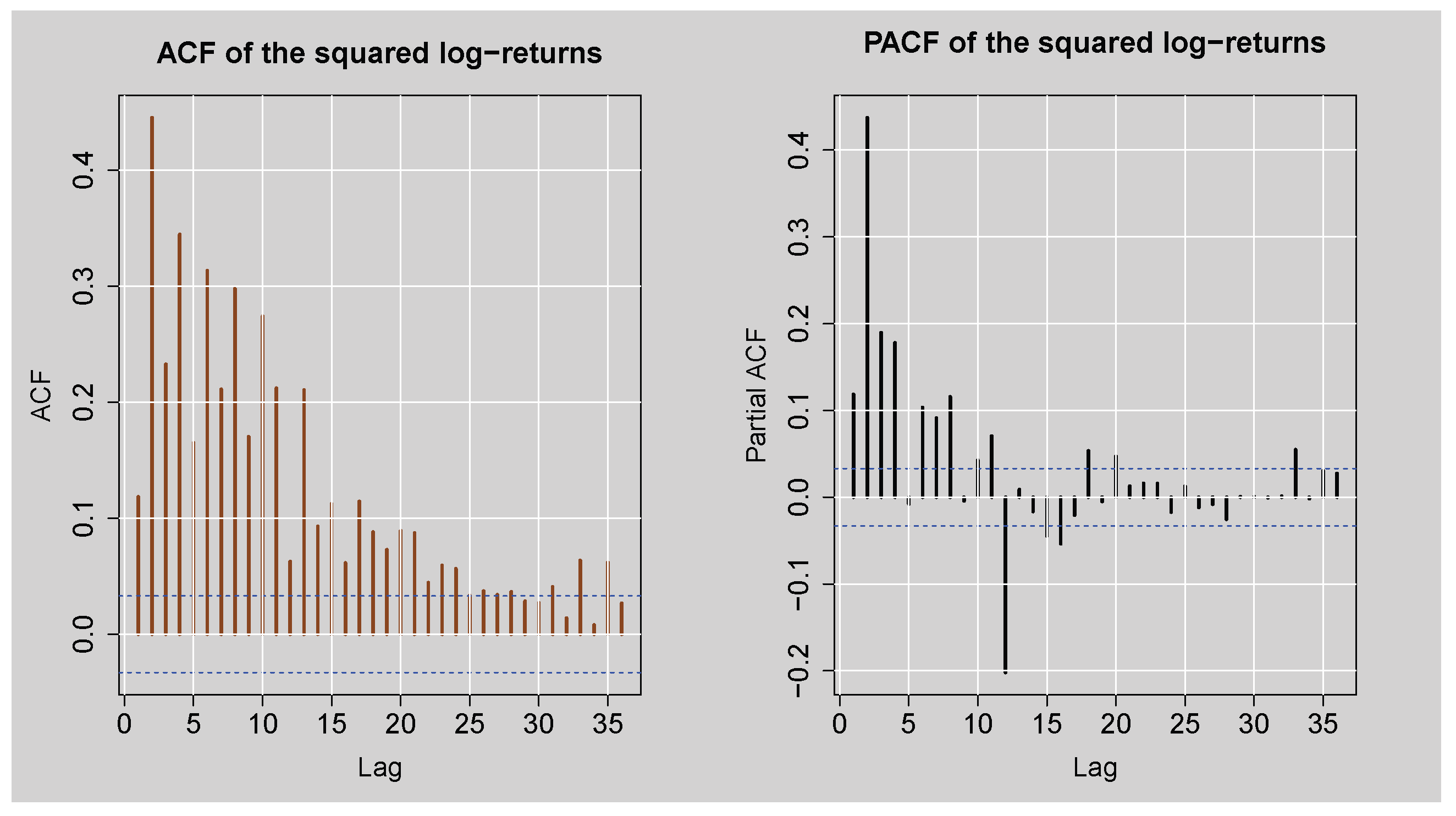
Figure 7.
Time series plot of the Residuals from ARMA(3,2) model.
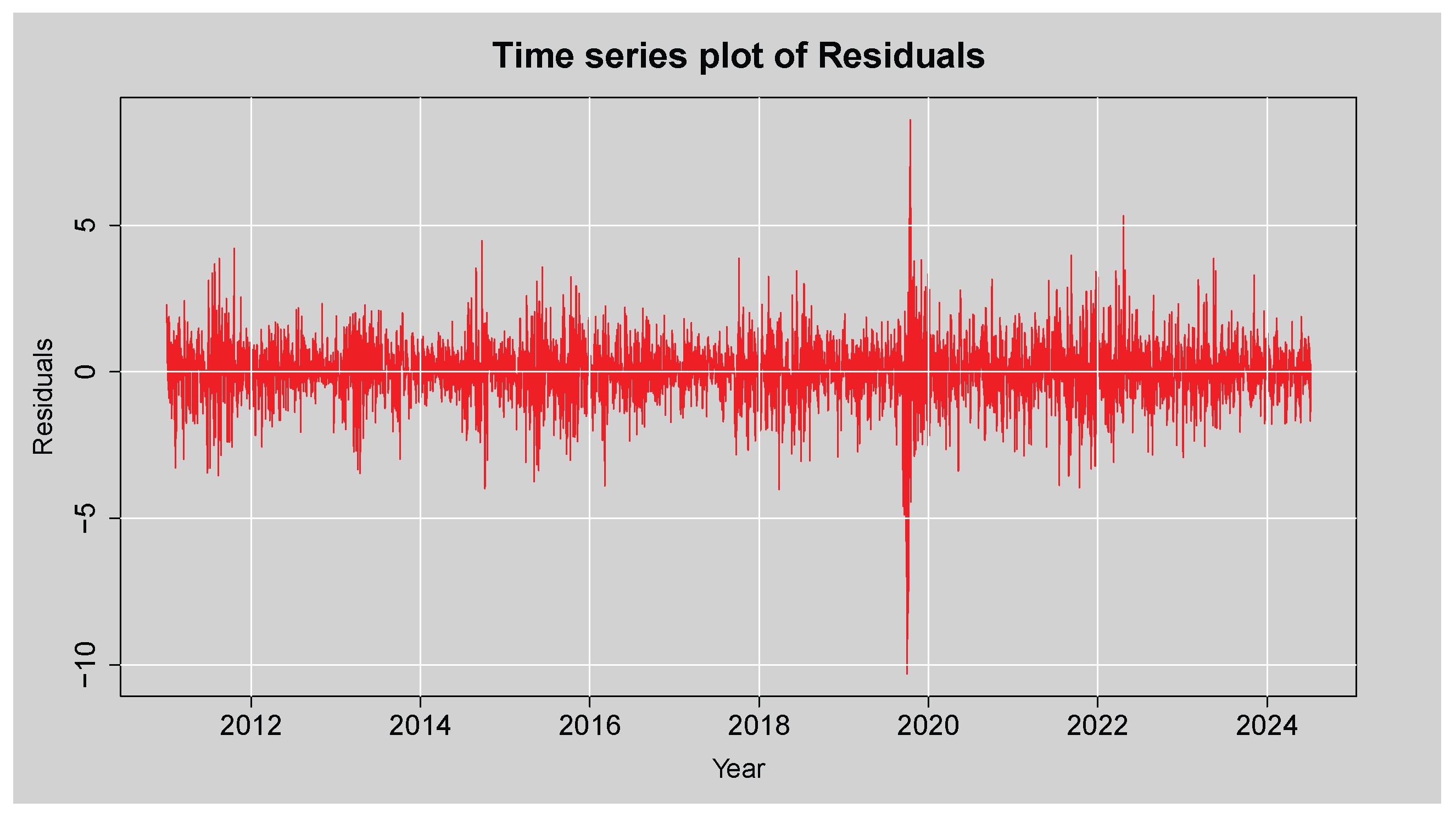
Figure 8.
ACF and PACF plots of the Residuals from ARMA(3,2) model.
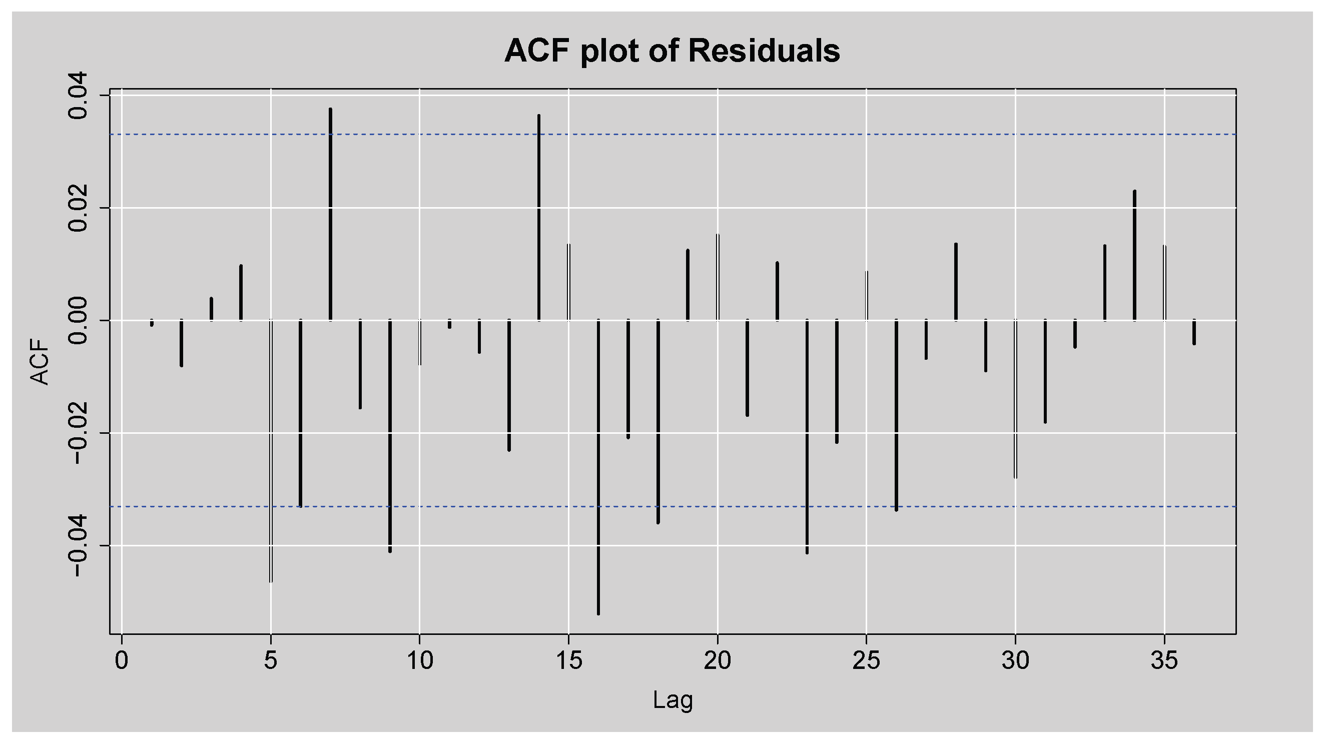
Figure 9.
Histogram and Normal Q-Q plots of the Residuals from ARMA(3,2) model.
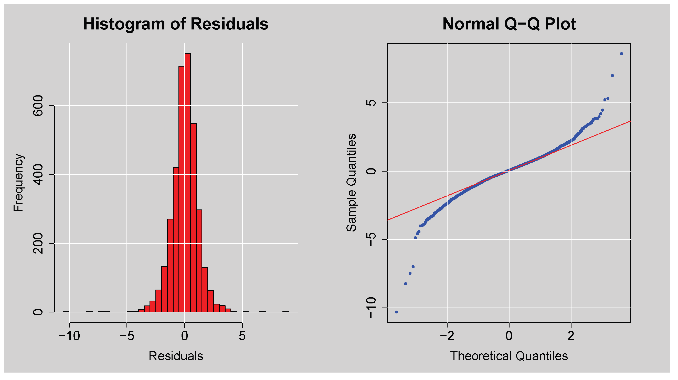
Figure 10.
Time series plot of the Squared Residuals from ARMA(3,2) model.
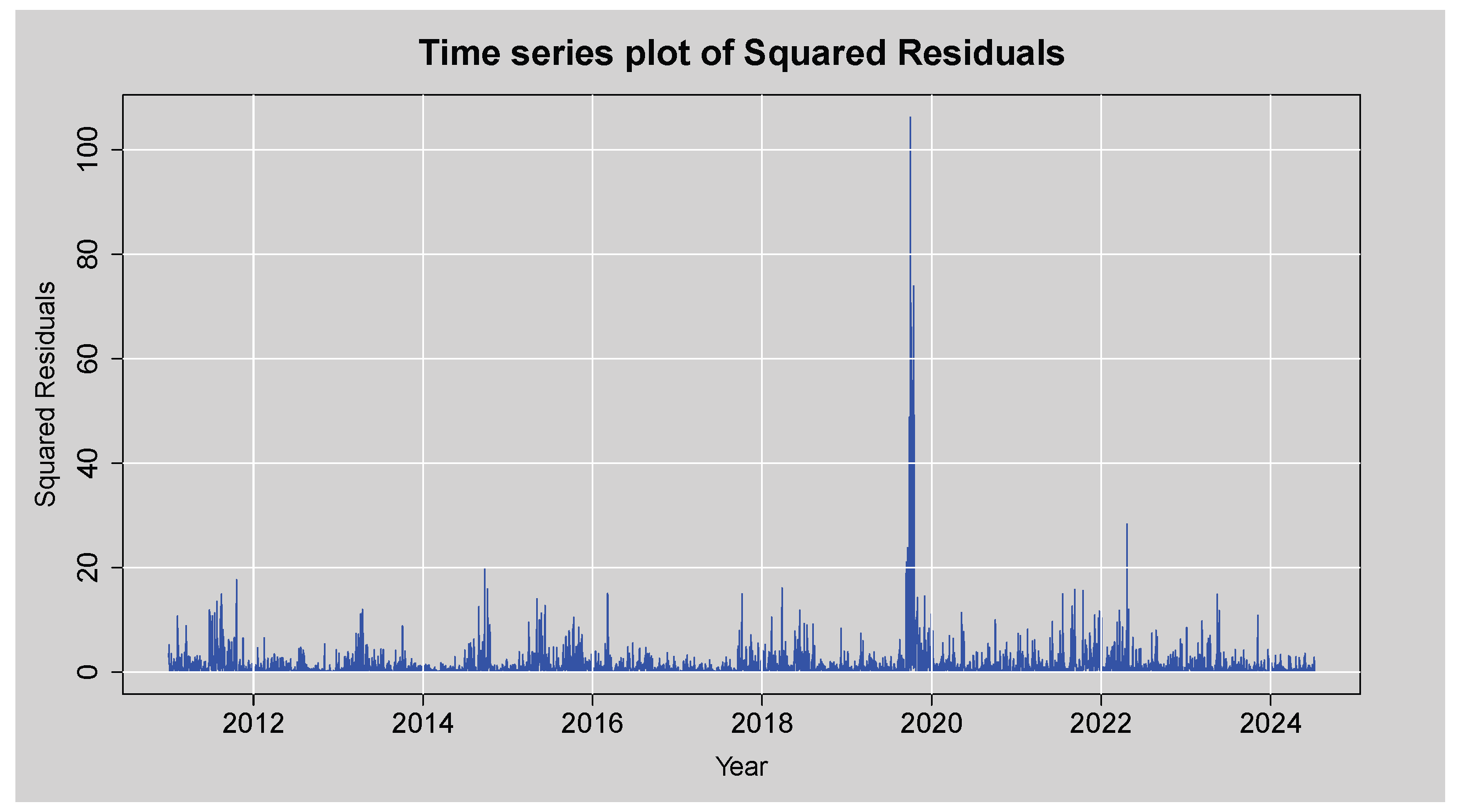
Figure 11.
ACF plot of the Squared Residuals from ARMA(3,2) model.
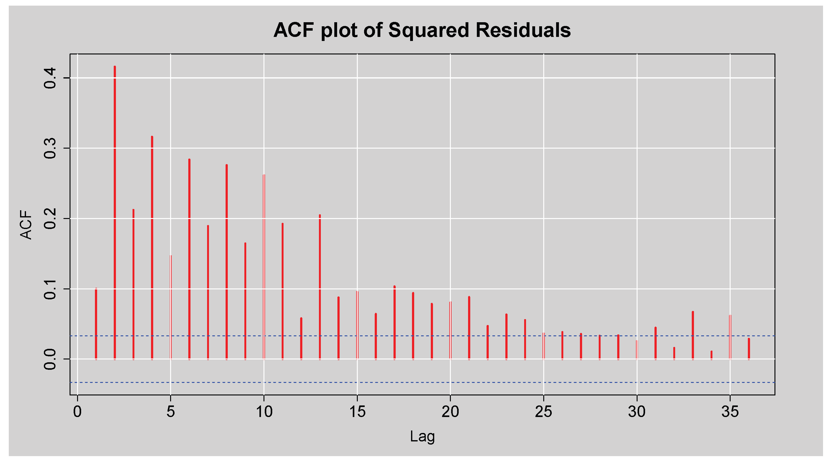
Figure 12.
ACF plot of the Standardised Residuals from ARMA(3,2)-EGARCH(1,1) model.
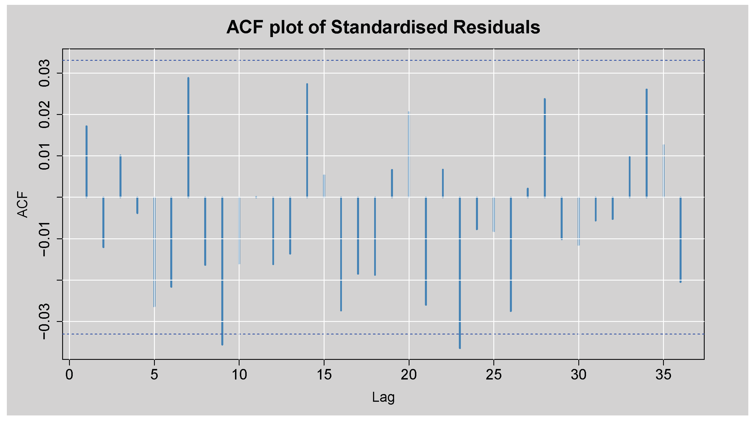
Figure 13.
ACF plot of the Squared Standardised Residuals from ARMA(3,2)-EGARCH(1,1) model.
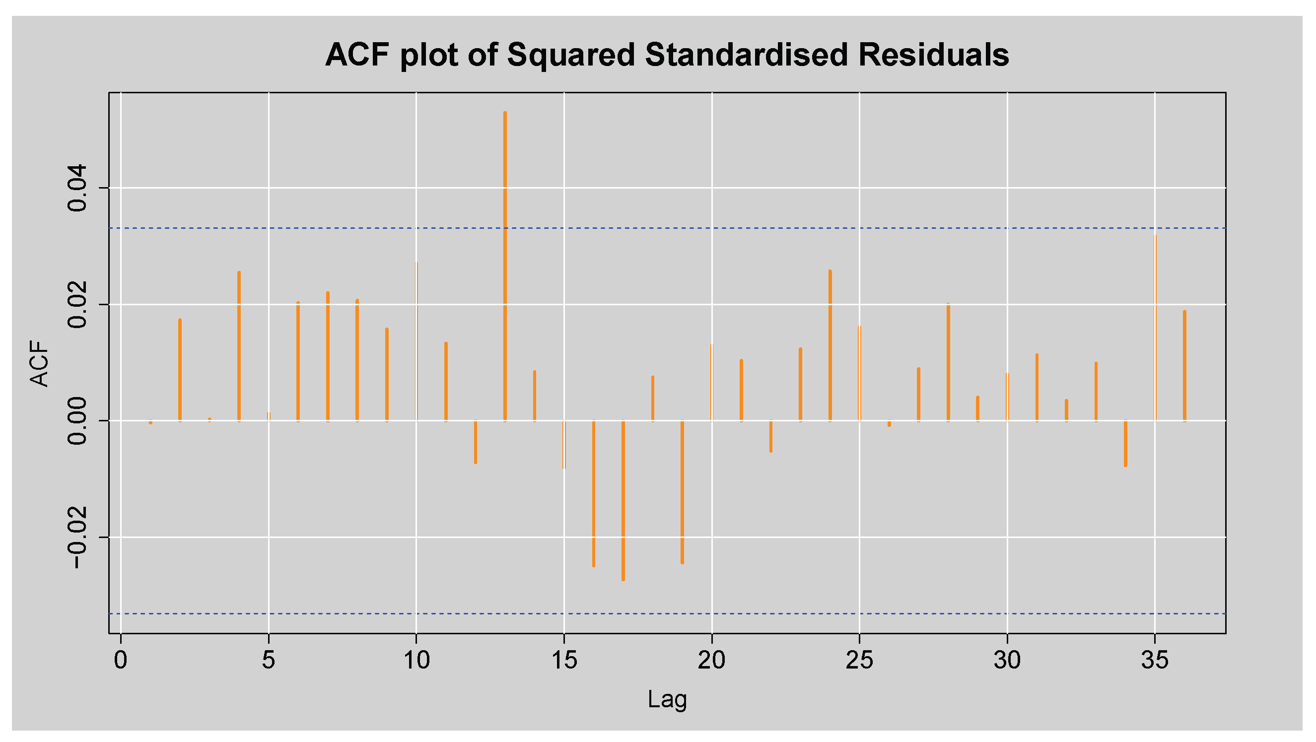
Figure 14.
Q-Q and Empirical Density plots of the Standardised Residuals from ARMA(3,2)-EGARCH(1,1) model.
Figure 14.
Q-Q and Empirical Density plots of the Standardised Residuals from ARMA(3,2)-EGARCH(1,1) model.
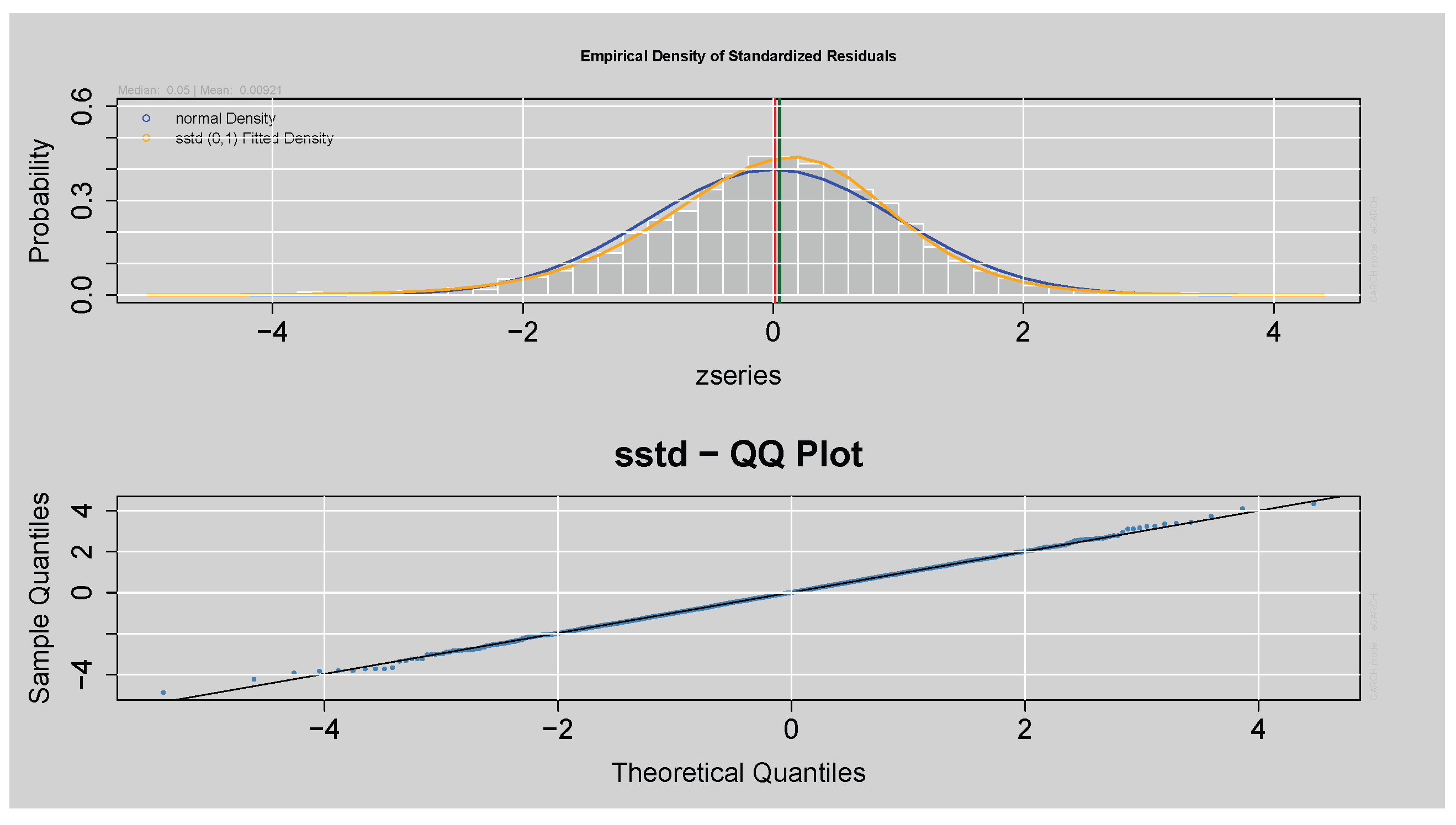
Figure 15.
News Impact Curve.
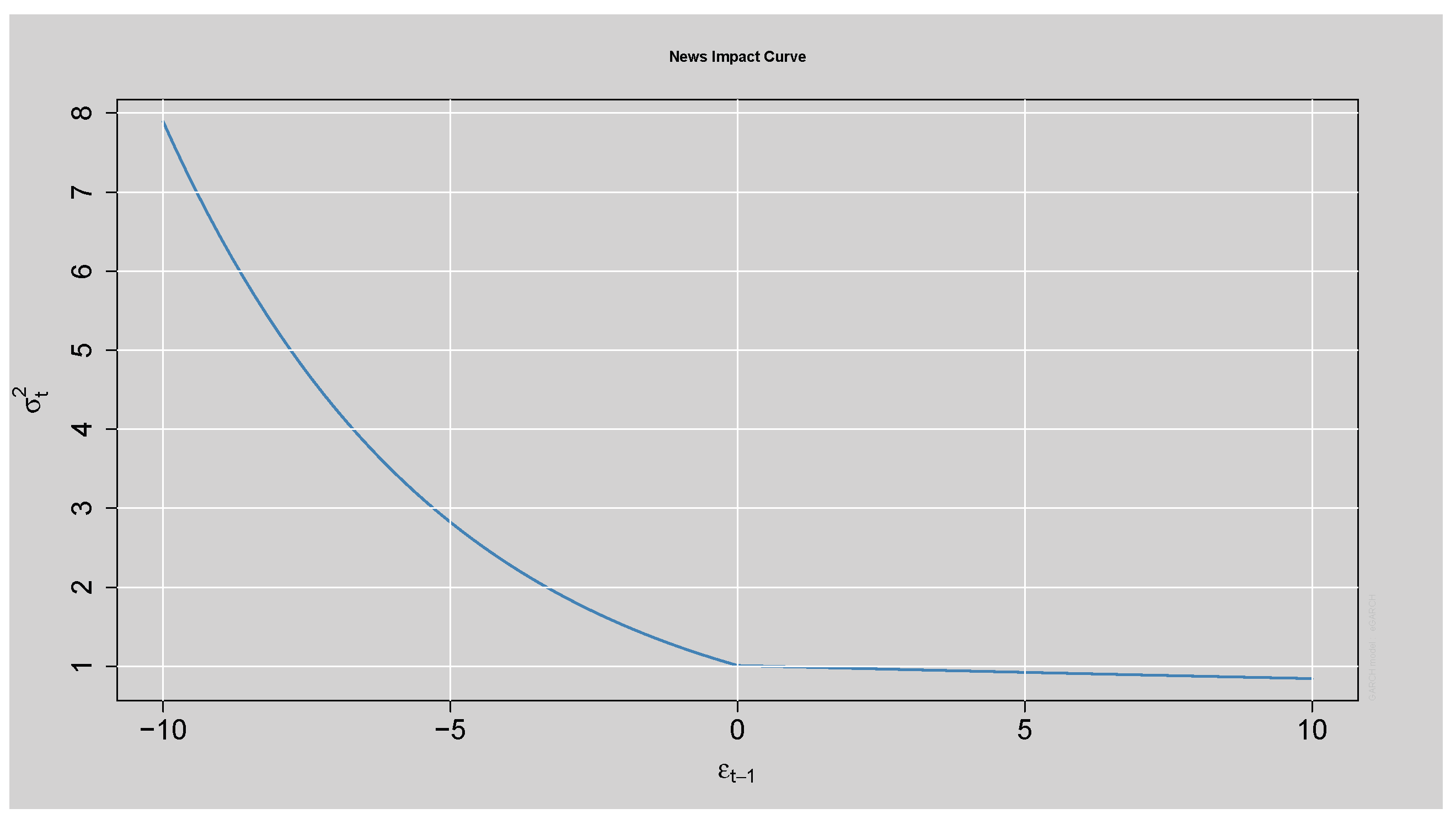
Figure 16.
Forecast of Standardised Residuals with 90% Prediction Intervals from the ARMA(3,2)-EGARCH(1,1)-XGBoost Model.
Figure 16.
Forecast of Standardised Residuals with 90% Prediction Intervals from the ARMA(3,2)-EGARCH(1,1)-XGBoost Model.
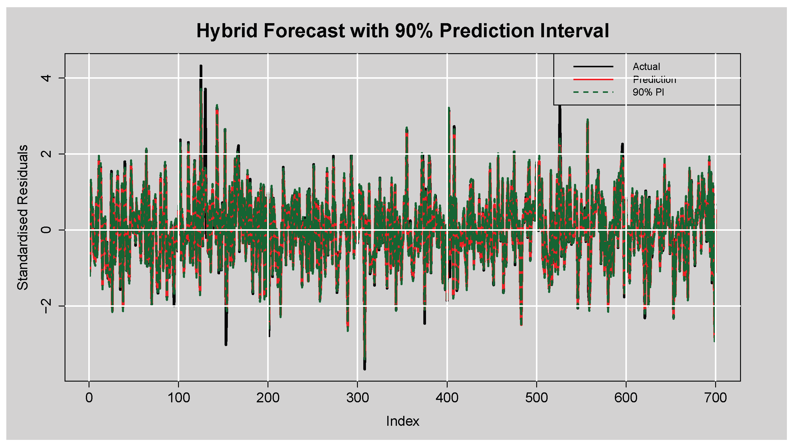
Figure 17.
Forecast of Standardised Residuals with 95% Prediction Intervals from the ARMA(3,2)-EGARCH(1,1)-XGBoost Model.
Figure 17.
Forecast of Standardised Residuals with 95% Prediction Intervals from the ARMA(3,2)-EGARCH(1,1)-XGBoost Model.
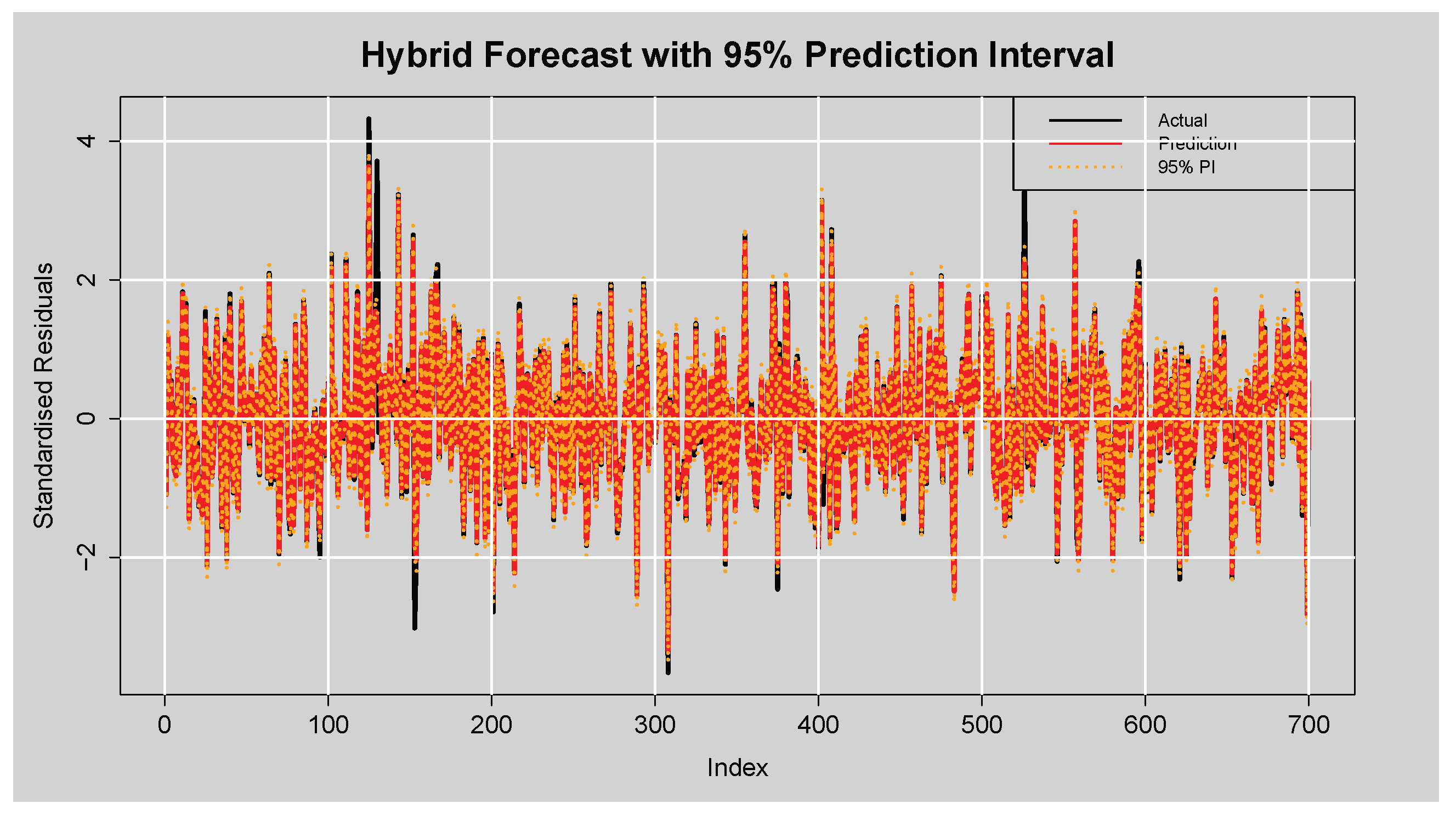
Figure 18.
Forecast of Standardised Residuals with 99% Prediction Intervals from the ARMA(3,2)-EGARCH(1,1)-XGBoost Model.
Figure 18.
Forecast of Standardised Residuals with 99% Prediction Intervals from the ARMA(3,2)-EGARCH(1,1)-XGBoost Model.
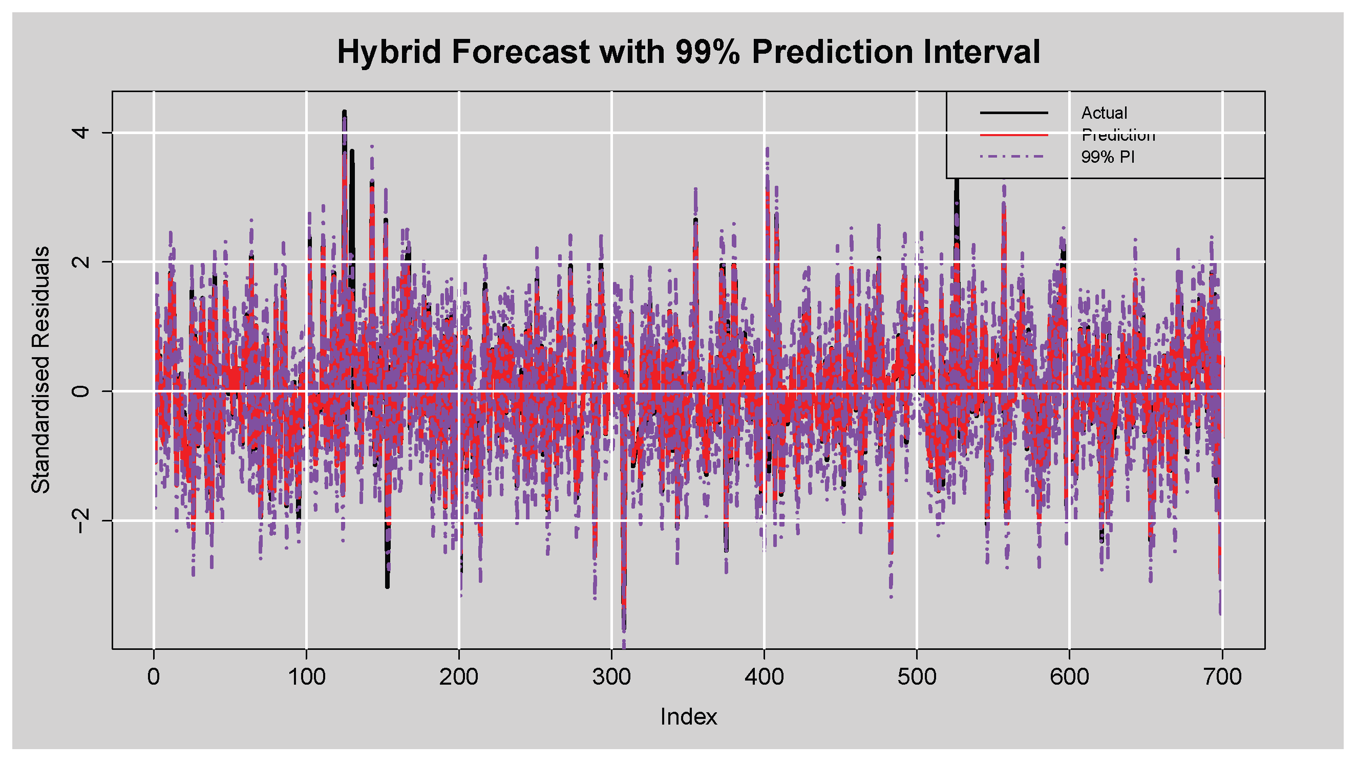
Figure 19.
Time-Varying Forecast Errors plot.
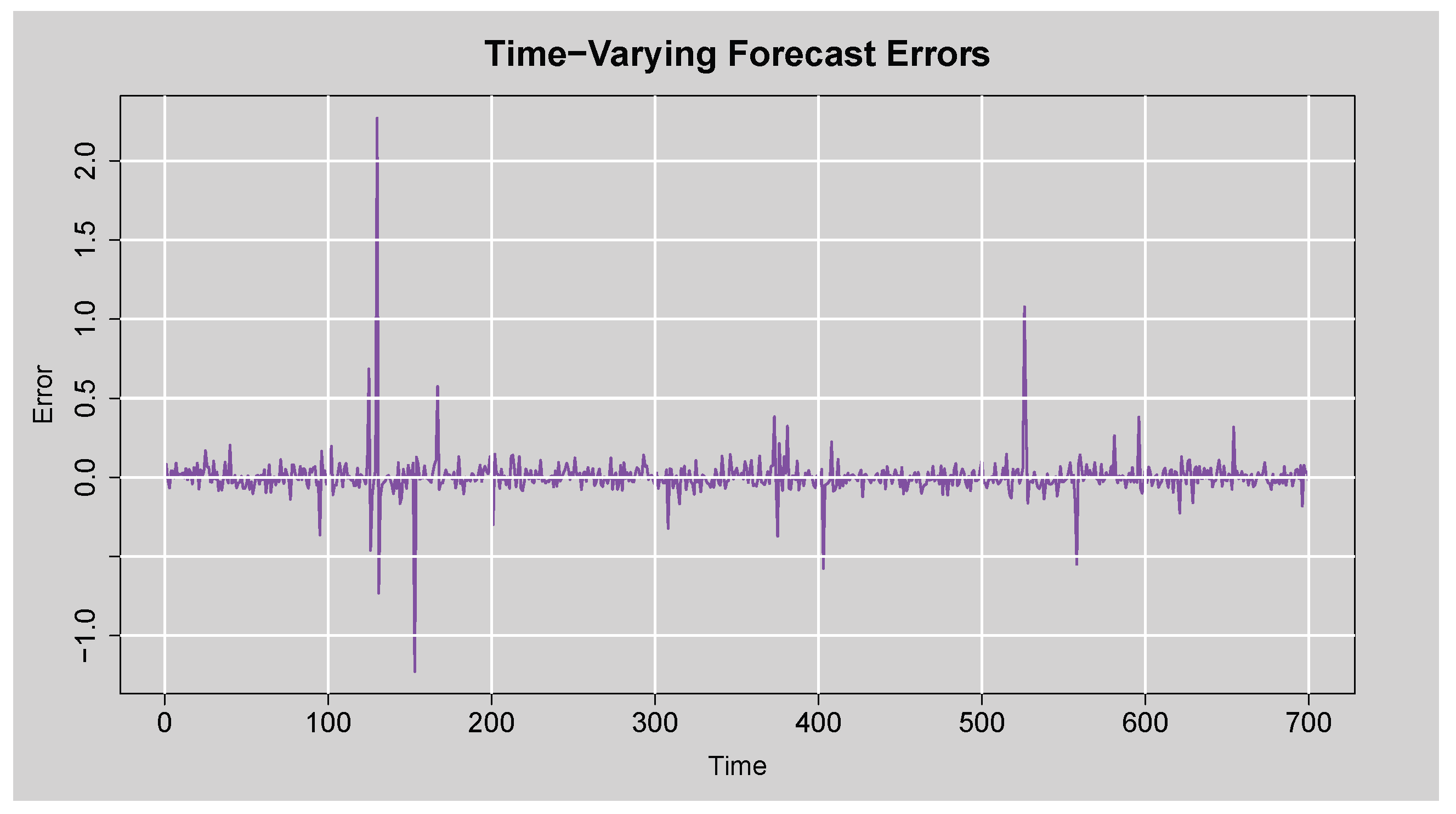

Table 1.
Results of the Box-Ljung Q test for autocorrelation detection.
| Lag | Statistic | Critical value | p-value |
|---|---|---|---|
| 10 | |||
| 15 | |||
| 20 | |||
| 25 | |||
| 30 | |||
| 35 |
Table 2.
Results of the Engle’s ARCH LM test for heteroscedasticity detection.
| Lag | Statistic | Critical value | p-value |
|---|---|---|---|
| 10 | |||
| 15 | |||
| 20 | |||
| 25 | |||
| 30 | |||
| 35 |
Table 3.
Summary of stationarity and normality tests for the log-returns.
| Test | Statistic | p-value | Conclusion | Decision |
|---|---|---|---|---|
| ADF | Reject H0 | Stationary | ||
| KPSS | Fail to reject H0 | Stationary | ||
| JB | Reject H0 | Not normally distributed |
Table 4.
Summary statistics of the log-returns.
| Min | Mean | Max | SD | Skew | Kurt | |||
|---|---|---|---|---|---|---|---|---|
Table 5.
Box-Lyung and JB test on the ARMA(3,2) Residuals.
| Lag | Statistic | p-value |
|---|---|---|
| 10 | ||
| 15 | ||
| 20 | ||
| 25 | ||
| 30 | ||
| 30 | ||
Table 6.
Engle’s ARCH LM test on the ARMA(3,2) Residuals.
| Lag | Statistic | p-value |
|---|---|---|
| 10 | ||
| 15 | ||
| 20 | ||
| 25 | ||
| 30 |
Table 7.
Box-Ljung test on the ARMA(3,2) Squared Residuals.
| Lag | Statistic | p-value |
|---|---|---|
| 10 | ||
| 15 | ||
| 20 | ||
| 25 | ||
| 30 |
Table 8.
Evaluation metrics for ARMA(3,2)–GARCH-type models under different conditional distributions.
Table 8.
Evaluation metrics for ARMA(3,2)–GARCH-type models under different conditional distributions.
| Conditional Distributions | ||||||
|---|---|---|---|---|---|---|
| Model | STD | SSTD | GED | SGED | GHD | |
| ARMA(3,2)-sGARCH(1,1) | AIC | |||||
| BIC | ||||||
| HQIC | ||||||
| LL | ||||||
| ARMA(3,2)-EGARCH(1,1) | AIC | |||||
| BIC | ||||||
| HQIC | ||||||
| LL | ||||||
| ARMA(3,2)-GJR-GARCH(1,1) | AIC | |||||
| BIC | ||||||
| HQIC | ||||||
| LL | ||||||
Table 9.
Box-Lyung test on the ARMA(3,2)-EGARCH(1,1) Standardised Residuals.
| Lag | Statistic | p-value |
|---|---|---|
| 1 | ||
| 14 | ||
| 24 |
Table 10.
Engle’s ARCH LM test on the ARMA(3,2)-EGARCH(1,1) Standardised Residuals.
| Lag | Statistic | p-value |
|---|---|---|
| 3 | ||
| 5 | ||
| 7 |
Table 11.
Box-Ljung test on the ARMA(3,2)-EGARCH(1,1) Squared Standardised Residuals.
| Lag | Statistic | p-value |
|---|---|---|
| 1 | ||
| 5 | ||
| 9 |
Table 12.
Sign Bias Test Results.
| t-value | p-value | |
|---|---|---|
| Sign Bias | ||
| Negative Sign Bias | ||
| Positive Sign Bias | ||
| Joint Effect |
Table 13.
Parameter Estimates of the ARMA(3,2)-EGARCH(1,1) model.
| Parameter | Estimate | p-value |
|---|---|---|
Table 14.
First 10 Forecast Results from the Hybrid ARMA(3,2)-EGARCH(1,1)-XGBoost Model.
| Actual | Prediction |
|---|---|
Table 15.
Forecast Accuracy Measure Results from the Hybrid ARMA(3,2)-EGARCH(1,1)-XGBoost Model.
| Forecast Accuracy Measures | ||||
|---|---|---|---|---|
| MASE | RMSE | MAE | MAPE(%) | sMAPE(%) |
Table 16.
Evaluation Metrics of the Prediction Intervals
| Evaluation Metrics | ||||
|---|---|---|---|---|
| PINC(%) | PICP(%) | PINAW(%) | PICWA(%) | PINAD(%) |
Disclaimer/Publisher’s Note: The statements, opinions and data contained in all publications are solely those of the individual author(s) and contributor(s) and not of MDPI and/or the editor(s). MDPI and/or the editor(s) disclaim responsibility for any injury to people or property resulting from any ideas, methods, instructions or products referred to in the content. |
© 2025 by the authors. Licensee MDPI, Basel, Switzerland. This article is an open access article distributed under the terms and conditions of the Creative Commons Attribution (CC BY) license (http://creativecommons.org/licenses/by/4.0/).
Copyright: This open access article is published under a Creative Commons CC BY 4.0 license, which permit the free download, distribution, and reuse, provided that the author and preprint are cited in any reuse.


