Submitted:
02 August 2025
Posted:
04 August 2025
Read the latest preprint version here
Abstract
Phytoplankton community composition (PCCs) - also referred to as functional groups play a key role in ocean biogeochemical cycling, climate regulation, and marine ecosystem dynamics. Accurate quantification of these groups from satellite ocean color data remains challenging due to spectral similarities among phytoplank- ton types and the limitations of existing empirical and semi-analytical models. In this study, we used an extreme gradient boosting (XGBoost) tree-based regression model to retrieve multiple PCCs and total chlorophyll-a concentrations from sim- ulated hyperspectral remote sensing top-of-atmosphere (TOA) ocean color data as well as some ancillary data. The intent is to mimic what could be gathered from the NASA Plankton, Aerosol, Cloud, ocean Ecosystem (PACE) mission and auxiliary data sources to characterize to characterize the environment. In its final form, the model, validated on an out-of-sample set, demonstrated strong predictive performance across most functional groups, with R2 values exceeding 0.95. Dinoflag- ellate retrievals showed lower accuracy (R2 = 0.53). Further analysis revealed that temperature was a key predictor alongside hyperspectral TOA radiance, suggesting that integrating external temperature data could enhance future retrieval models. Furthermore, despite using only 10% of the available hyperspectral bands, feature importance analysis showed that specific spectral regions disproportionately con- tributed to model predictions. These findings highlight the potential of machine learning for phytoplankton classification and inform future algorithm development for hyperspectral ocean color missions.
Keywords:
Phytoplankton
; Regression
; XGBoost
; Shap
; Explainable AI
1. Introduction
Phytoplankton community composition (PCCs) play a fundamental role in marine biogeochemical cycles, influencing carbon sequestration, nutrient fluxes, and global climate feedbacks. Different functional groups contribute uniquely to these processes; for example, diatoms facilitate carbon export through rapid sinking, cyanobacteria fix atmospheric nitrogen, and coccolithophores regulate carbonate chemistry via calcification (Marañón and Cermeño P. 2014; Boyd and Doney 2002). Identifying and quantifying these groups from space is crucial for understanding their ecological functions, detecting environmental changes, and improving ocean biogeochemical models (Bopp et al. 2005; Laufkötter et al. 2016). However, current satellite ocean-color products primarily provide total chlorophyll a concentrations, which do not directly indicate community composition. To address this gap, various remote sensing algorithms have been developed to infer phytoplankton diversity, each with limitations in distinguishing certain groups and quantifying their biomass accurately (Mouw et al. 2017).
1.1. Remote Sensing Approaches for PCC Retrieval
Phytoplankton classification from satellite remote sensing has traditionally relied on empirical and semi-analytical methods. Empirical band-ratio techniques, such as PHYSAT, classify dominant phytoplankton groups based on anomalies in spectral reflectance but are often region-specific and limited to broad functional classes (Alvain et al. 2005, 2008). Semi-analytical models, in contrast, use inherent optical properties (IOPs) to infer phytoplankton composition from satellite reflectance, providing a more mechanistic approach (Hirata et al. 2011). Hybrid models incorporate additional environmental variables, such as sea surface temperature and total chlorophyll, to infer community structure (Brewin et al. 2010).
Hyperspectral ocean-color sensors, such as NASA’s Plankton, Aerosol, Cloud, ocean Ecosystem (PACE) mission, may have the potential to improve PCC retrieval by capturing finer spectral features associated with phytoplankton pigments (Dierssen et al. 2023). That is not to say that hyperspectral resolution is sufficient on its own. Optical similarity between different groups, depth-related biases in surface measurements, as well as associated measurement uncertainties inherenth to the noisy marine environment will likely hinder retrieval accuracy (IOCCG 2014). Most current models either estimate phytoplankton size classes or assign a single dominant group per pixel, often failing to capture the complexity of mixed communities (Ciotti, Lewis, and Cullen 2002).
1.2. Study Contribution and Approach
In this study, we use a scalable, high-performance ensemble learning algorithm; extreme gradient boosting (XGBoost) (Chen and Guestrin 2016) to identify phytoplankton community composition from satellite ocean color data. The ensemble aspect of this algorithm makes it more resistant to overfitting. XGBoost is less opaque than neural networks. Finally, XGBoost is robust to data issues that are problematic for other machine learning models such as Neural Networks, including highly correlated (spectral) data or data of varying scales.
XGBoost outperformed alternative approaches in applications such as harmful algal bloom detection (Izadi et al. 2021) and phytoplankton biomass estimation (Yan et al. 2025), which highlight the suitability of the approach1 for remote sensing applications. Our work aligns with the objectives of the PACE mission by contributing an advanced classification algorithm that enhances hyperspectral monitoring of phytoplankton diversity (Zhang et al. 2024). To our knowledge, this is the first application of XGBoost for PCC classification in ocean color remote sensing, offering a robust alternative to traditional retrieval methods.
Our approach was to leverage a large dataset of simulated hyperspectral TOA radiance and associated environmental variables to improve both the discrimination of functional groups and the quantification of their biomass. Previous remote sensing algorithms often classified only a dominant PCC or broad size class (Mouw et al. 2017) and relied on empirical band relationships that lacked generalizability (Hirata et al. 2011). By utilizing a machine learning framework capable of integrating multiple features, our approach reduces classification errors and enhances retrieval precision. Moreover the application of eXplainable AI (XAI) techniques to relate predictions to their input may further guide future efforts to improve PCC quantification.
2. Methods
2.1. Data Preparation and Feature Selection
We utilized a simulated dataset representing the world ocean over 31 days, corresponding to December 2021. The simulation generated hyperspectral remote sensing TOA radiance data, emulating a sensor configuration akin to that of the PACE instrument. Due to the high dimensionality of the original spectral data, we conducted an initial exploratory analysis and observed strong correlations among many of the channels. To reduce redundancy while preserving essential spectral information, we retained 51 channels by selecting one channel every ten. Note that despite this feature subsampling, spectral features are characterized by high degree of correlation we opted against applying principal component analysis for two principal reasons. The first reason is to avoid overemphasizing blue water signal contributed by the extensive oceanic regions present in a global satellite scene, and which could mask coastal processes of interest. The second reason is that tree-based algorithms such as XGBoost are resiliant to input multicollinearity. To further contextualize the ocean color signal, we also included auxiliary environmental variables such as temperature and latitude. Though not available from actual PACE measurements, climatology including temperature could be readily sourced elsewhere to augment observations on hand.
The dataset was divided into training and test sets using an 80/20 split. The training set was exclusively used for model development and hyperparameter optimization (see next section), while the test set was set aside until the final validation of model performance.
2.2. Model Choice
We employed an XGBoost Regressor model with a multi-output regression head to predict simultaneously multiple phytoplankton functional groups as well as total chlorophyll-a concentration. XGBoost is a high-performance, scalable implementation of gradient boosting that has become a popular choice for a wide range of regression and classification tasks (Chen and Guestrin 2016). This approach consists in building an ensemble of decision trees sequentially, where each new tree attempts to correct the errors made by the previous trees. By optimizing a regularized objective function, XGBoost effectively controls overfitting while enhancing prediction accuracy. Its efficient handling highly correlated data, support for parallel computation, and flexible regularization mechanisms make it particularly well-suited for complex modeling tasks.
2.3. Hyperparameter Optimization and Model Training
Given the complexity of the problem and the high dimensionality of the input features, it was critical to optimize the hyperparameters to achieve robust performance and prevent overfitting. To this end, we conducted hyperparameter optimization using the Optuna library (Akiba et al. 2019). Specifically, we employed the efficient Tree-structured Parzen Estimator (TPE) algorithm (Bergstra et al. 2011). TPE is a Bayesian optimization method that iteratively builds probabilistic models of the hyperparameter space based on past evaluation results. By modeling the distributions of promising and less promising hyperparameter configurations, TPE suggests new parameter sets to explore, focusing the search on regions likely to yield improved performance. To further enhance the efficiency of the optimization process, we utilized Optuna’s MedianPruner with n_warmup_steps=5. This pruner automatically stops unpromising trials during the early stages of training (after at least 5 steps) if their intermediate results indicate they are unlikely to outperform the median performance of completed trials. The optimization step used an objective function to minimize the root mean squared error (RMSE) computed via three-fold cross-validation on the training set. The hyperparameters under investigation are lthe learning rate, maximum tree depth, number of estimators, subsample ratio, column subsample ratio, and gamma (the minimum loss reduction required to make a further partition on a leaf node); cf Table 1 for further details. The Bayesian optimization procedure allowed us to efficiently explore the hyperparameter space by leveraging past trial information to prune unpromising candidate parameter sets early, thereby reducing overall computational cost.
Once the optimization step complete, we instantiated the XGBoost model with the best set of hyperparameters and trained it on the full training set.
2.4. Sensitiviy Analysis to Spectral Resolution through Band Downsampling
To assess the impact of spectral resolution on model performance, we conducted a sensitivity analysis by subsampling the hyperspectral input data to approximate the band configurations of MODIS and VIIRS sensors. Specifically, we selected the closest available channels in our simulated dataset to match the central wavelengths of MODIS and VIIRS ocean color bands (limited to <750 nm), while retaining temperature as an auxiliary predictor. For both sensor configurations, we trained new models using the original set of hyperparameters optimized for the full hyperspectral dataset. This approach enabled a controlled comparison in which only the input features were varied, allowing us to isolate the impact of reduced spectral resolution on predictive skill. The same train/test split used in the initial model development was retained to ensure comparability of performance metrics across configurations, with the goal of measuring sensitivity rather than generalizability.
2.5. Model Evaluation and eXplainable AI (XAI)
Once the optimal hyperparameter combination was identified, we retrained the final XGBoost model on the full training set using these optimized settings. Finally, we evaluated the performance of the retrained model on the held-out test set to assess its generalizability.
2.5.1. Prediction Explainability
To enhance interpretability and gain insights into how different input features influence model predictions, we employed Shapley Additive Explanations (SHAP), a widely used explainable AI (XAI) framework for interpreting complex machine learning models. SHAP is named after the concept of Shapley values, which consists in assigning importance values to each input feature by estimating its contribution to the model’s predictions across different samples. The method is rooted in cooperative game theory, and guarantees a fair distribution of importance scores among features (Lundberg and Lee 2017).
Given the computational complexity of our XGBoost model and the high dimensionality of the dataset, we conducted SHAP analysis on a random subsample of 10,000 observations from the test set. This subset was selected to balance computational feasibility while maintaining a representative sample of phytoplankton spectral diversity.
We generated SHAP summary plots, which provide a comprehensive visualization of feature importance and the directionality of their influence on model outputs. These plots display the magnitude of each feature’s impact across all predictions, helping to identify the most influential spectral and environmental variables in determining phytoplankton functional group composition. The insights gained from SHAP analysis aid in validating model behavior and ensuring its ecological plausibility.
2.5.1.1. Code Availability
All analysis and modeling code used in this study was written in Python 3.12. This code is publicly available on GitHub.
3. Results
3.1. Hyperparameter Optimization (HPO)
We performed hyperparameter optimization using a Bayesian optimization framework implemented with Optuna. The metric used for optimization was the average RMSE (in units of ) computed over the cross-validation folds and across all target compartments. The “full HPO run” best parameters indicate a relatively aggressive model, characterized by deep trees with many estimators, a moderate learning rate, and little regularization via gamma.
The best trial finished with an RMSE of . Below is the list of hyperparameters researched, the optimal values found, and an interpretation of these values:
- Learning Rate (learning_rate): - This moderate learning rate suggests the model takes reasonably sized steps when updating that are neither too aggressive (which might lead to overshooting the optimum) nor too conservative (which could slow down convergence).
- Max Depth (max_depth): 10 - A depth of 10 allows the trees to capture complex interactions. This may indicate that the data has non-linear relationships that benefit from deeper trees. Such a depth can be associated with overfitting. The cross-validation process during HPO should minimize this however.
- Number of Estimators (n_estimators): 466 -Building around 466 trees indicates the ensemble haa to tackle inherent complexity in the data that was not apparetn during the Exploratory Data Analysis phase. A larger number of trees generally improves performance—up to a point before overfitting becomse a risk. This number in conjunction with the cross validation process suggest this number strikes a balance between performance and overfitting.
- Subsampling (subsample): - This indicates each of the 466 trees is using roughly 66% of the data. This introduces randomness that helps prevent overfitting as not all samples in any cross-validation fold are used to build every tree.
- Features used per tree (colsample_bytree): - Using about 89% of the features per tree indicates that most features are informative, and the model is allowed to consider almost the full feature set at each split. - See features used in the Methods section.
- Gamma (gamma): - An extremely low gamma value means that almost no minimum loss reduction is required to make a split. This implies that the algorithm will split more readily, potentially capturing fine details. Awareness of this hyperparameter values is important as low gamma can risk overfitting.
3.2. Optimized Model Validation
The next step was to load the best set of hyperparameter (listed above) into the model and retrain the model on the entire training set. The optimized and trained model was then validated using the test set, which prior to the HPO process and until this step had been set aside.
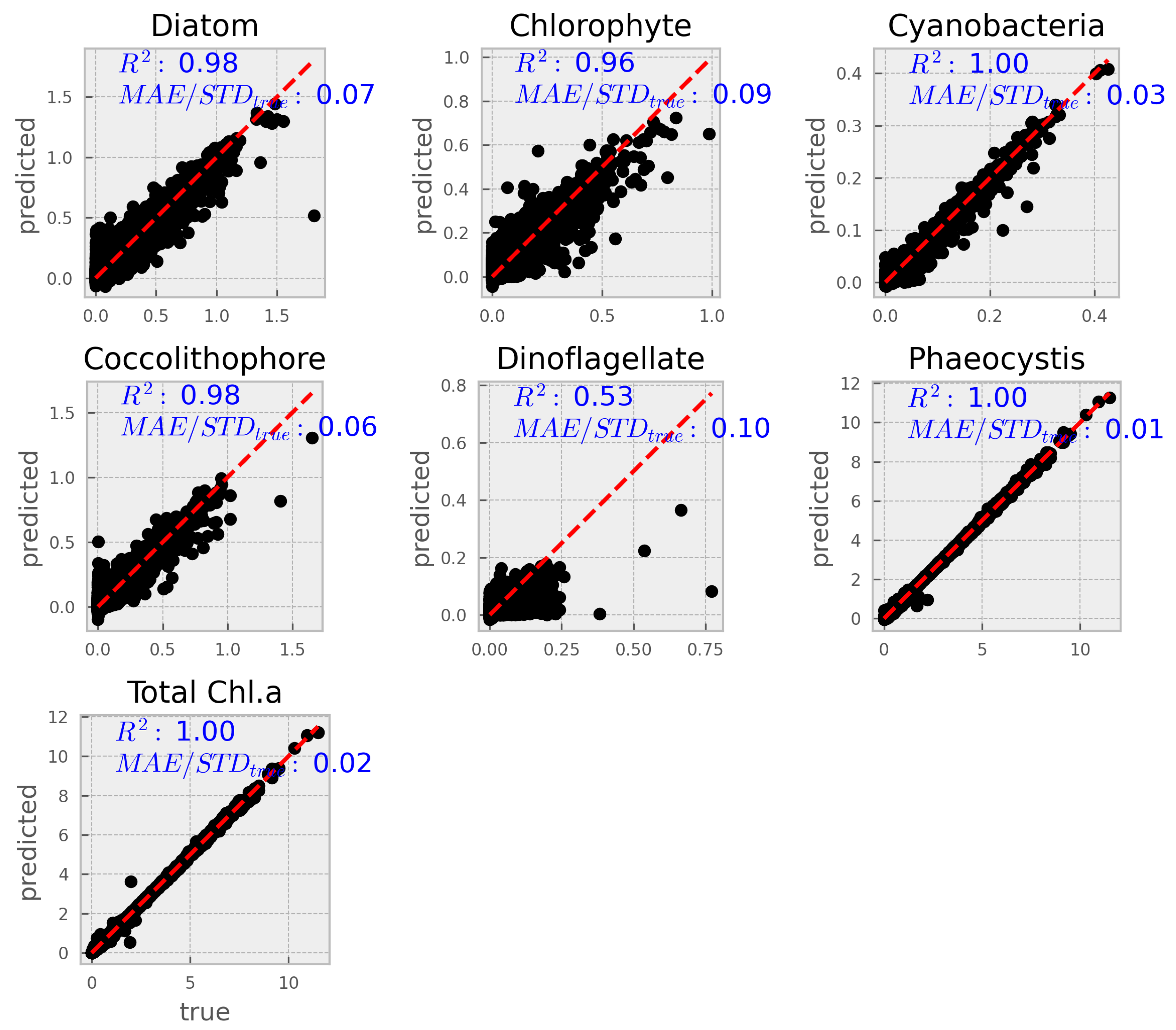
Figure 1.
Goodness-of-fit plots for all groups and total chorophyll a, measured on out-of-sample data set. THe model is able to predict with very good accuracy. Dinoflagellates are the notable exception.
Figure 1.
Goodness-of-fit plots for all groups and total chorophyll a, measured on out-of-sample data set. THe model is able to predict with very good accuracy. Dinoflagellates are the notable exception.
A more complete set of metrics are summarized in table Table 2 See further below for metrics explanation.
3.2.1. Explanation of metrics
-
Mean Squared Error (MSE):MSE is the average of the squared differences between the predicted and true values. Squaring the errors emphasizes larger deviations, making MSE sensitive to outliers. In our context, MSE is expressed in units of (mg L−1 Chla)2. Lower MSE values indicate better model performance.
-
Root Mean Squared Error (RMSE):RMSE is the square root of the MSE, bringing the error metric back to the original units (mg L−1 Chla). It provides a direct measure of the average prediction error magnitude. Lower RMSE values suggest that the model’s predictions are closer to the true values.
-
Mean Absolute Error (MAE):MAE calculates the average absolute difference between predicted and true values. Unlike MSE, it does not square the errors, so it is less sensitive to large outliers. MAE is also expressed in the same units as the target variable (mg L−1 Chla). A lower MAE indicates better predictive accuracy.
-
Coefficient of Determination (R-squared):R-squared measures the proportion of the variance in the dependent variable that is predictable from the independent variables. It ranges from 0 to 1, where a value closer to 1 indicates that the model explains a high proportion of the variance in the data. In our results, high R-squared values generally indicate strong model performance, although lower values (e.g., for dinoflagellates) suggest room for improvement.
-
MAE/StDevtrue:This ratio compares the mean absolute error to the standard deviation of the true values. It provides a relative measure of error by indicating how the average error compares to the inherent variability in the data. A lower ratio implies that the model’s prediction error is small relative to the natural variability of the observations.
3.3. XAI with Shapley Values
The SHAP summary plots provides insights into feature importance and their effects on model predictions for phytoplankton community composition.
Figure 2.
Shapley values are shown for each functional group and for total chlorophyll. Features are ranked by most to least impactful, from top to bottom. Only the top 6 predictive features are shown. Along the x-axis, positive SHAP values indicate a positive relationship with the predicted; negative values, a negative one. Wider sections indicate greater variability. The color gradient represents feature values, with red for high values and blue for low values. The midpoint of the color bar reflects a percentile-based central value, not necessarily the mean, median, or mode, as it depends on the feature’s distribution.
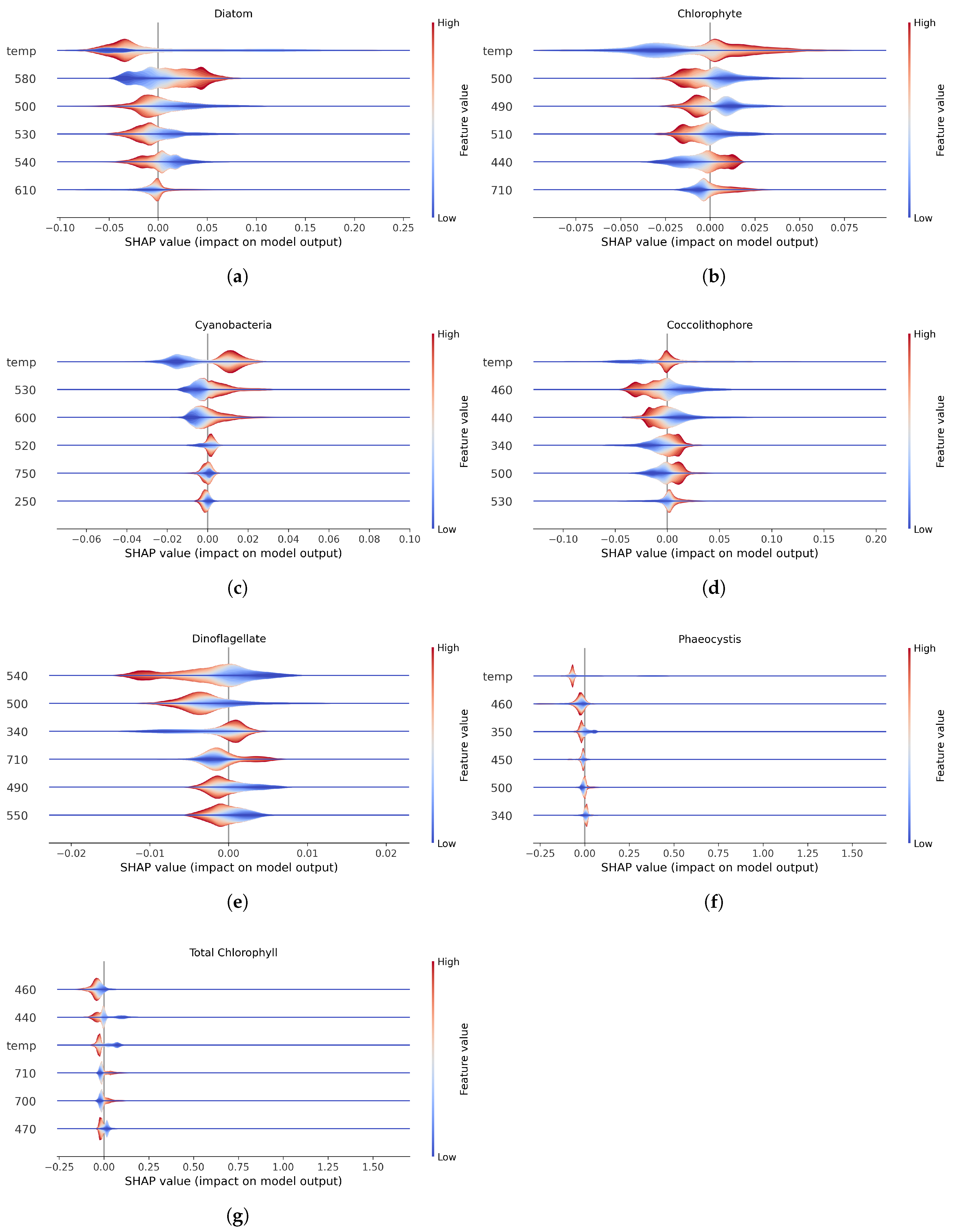
Most saliently, temperature was the top factor for all phytoplankton groups but is not a primordial feature in quantifying dinoflagellates.
3.4. Spectral Resolution Sensitivity Analysis
To evaluate the sensitivity of model performance to spectral input resolution, we conducted additional experiments using reduced-band versions of the input data, corresponding to the band configurations of the MODIS and VIIRS ocean color sensors. For each sensor-specific dataset, we selected the closest matching channels from the original simulated hyperspectral inputs (limited to <750 nm), while retaining temperature as an auxiliary predictor.
All modeling conditions—hyperparameters, training procedure, and the original 80/20 train-test split—were held constant to isolate the effect of spectral resolution. Model performance was evaluated using multiple regression metrics across PCCs, including diatoms, chlorophytes, cyanobacteria, coccolithophores, dinoflagellates, and prasinophytes, as well as total chlorophyll-a.
Figure 3 summarizes the RMSE values for each model configuration. As expected, both band-limited models showed increased prediction error relative to the full hyperspectral model. The MODIS-band model exhibited an RMSE increase of 1.5–2.5× across most groups, with declines in R² particularly evident for diatoms, coccolithophores, and total chlorophyll. The VIIRS-band model showed consistently lower errors and higher explained variance than the MODIS counterpart, indicating better preservation of model skill under reduced spectral input.
To complement the aggregated metrics, Figures Figure 4 and Figure 5 show predicted versus true values for each group using the MODIS and VIIRS subsets, respectively. While both reduced models show reasonable alignment along the 1:1 line, greater scatter and bias are evident relative to the hyperspectral model, particularly for diatoms and dinoflagellates.
4. Discussion
The results presented here demonstrate that machine learning, particularly XGBoost, can effectively retrieve phytoplankton functional group (PCC) concentrations and total chlorophyll-a from hyperspectral top-of-atmosphere (TOA) data and auxiliary variables. The model performed well across most PCCs, with root mean squared error (RMSE) values under and values exceeding 0.95. The exception was dinoflagellates, which exhibited significantly lower predictive accuracy (), a result also reflected in their higher normalized MAE and MAPE values.
Feature importance analysis using SHAP values revealed that temperature was among the top six predictors for all groups except dinoflagellates, for which no strong dependence on any single environmental feature emerged. These patterns point to functional differences in ecological drivers between PCCs. In particular, the centrality of temperature for most groups highlights its role as a proxy for environmental gradients, biogeography, and metabolic scaling.
Dinoflagellates do not exhibit a single, well-defined biogeographical zone of dominance as do cyanobacteria (tropical oligotrophic waters), diatoms (high latitudes and upwelling systems) or coccolithophores (subpolar blooms) (Buitenhuis 2013; Gregg and Rousseaux 2019). Instead, they are often considered ecological opportunists, occupying a broad range of regions, particularly stratified, nutrient-depleted, and temperate to tropical environments (Smayda and Reynolds 2001; Kibler 2015). Their distribution is governed less by temperature per se than by water column stability, nutrient availability (especially high N:P conditions), and their ability to exploit mixotrophic strategies (Jeong 2010; P. M. et al. Glibert 2001; Flynn 2013). Several studies suggest that warming-driven increases in stratification may promote shifts from diatom- to dinoflagellate-dominated systems—not because dinoflagellates prefer warmer temperatures, but because they thrive in the low-nutrient, low-turbulence conditions that warming often produces (P. M. Glibert 2020; Peperzak 2003; Fu 2012).
These ecological patterns are further supported by physiological observations. Anderson et al. (Anderson et al. 2021) demonstrated that dinoflagellates exhibit shallower thermal performance curves compared to other PCCs, with lower maximum growth rates and broader thermal tolerance. In contrast, diatoms and cyanobacteria display distinct thermal optima and strong growth responses to temperature. This generalist thermal profile offers a plausible interpretation for temperature not being a dominant feature for dinoflagellate prediction in our model. Other important factors linked to their distribution, such as stratification, irradiance, and nutrient regime are only partially, or not at all, captured by the input features used here. The SHAP-based feature interpretation supports this ecological understanding and underscores the need to include more nuanced environmental predictors in future modeling efforts.
The strength of the model, particularly for diatoms, coccolithophores, and phaeocystis, suggests that important spectral and environmental signals are being captured despite substantial dimensionality reduction. This supports the feasibility of operational PCC retrieval using compressed hyperspectral data, especially when paired with interpretable machine learning models.
However, this study is based on simulated TOA radiance data, and real-world deployment will depend on atmospheric correction, instrument fidelity, and access to reliable ancillary predictors. Future work should validate the model on actual PACE observations and incorporate additional features—such as nutrient proxies, light attenuation, and mixed layer depth—to better capture ecological dynamics across all functional groups.
5. Conclusions
This study presents a novel, explainable machine learning framework for retrieving phytoplankton functional group concentrations from simulated hyperspectral top-of-atmosphere radiance data. Using an XGBoost model trained on reduced spectral features and auxiliary inputs such as temperature and latitude, we achieved high predictive performance across most functional groups and total chlorophyll-a. Model interpretation using SHAP values revealed that temperature was a key predictor for all groups except dinoflagellates, whose distribution appears to be driven by a broader suite of ecological factors such as stratification, nutrient limitation, and mixotrophy.
These findings reinforce the importance of tailoring remote sensing algorithms to the ecological and physiological diversity of phytoplankton groups. They also demonstrate that physically interpretable, high-performing models can be built even when using compressed hyperspectral inputs. However, the data tested is still simulated. Confirmation studies focusing on real sensor data (e.g., from the PACE mission) and incorporating additional oceanographic predictors to improve performance across all functional groups—especially those, like dinoflagellates, whose success is governed by indirect or emergent environmental conditions.
References
- Akiba, Takuya, Shotaro Sano, Toshihiko Yanase, Takeru Ohta, and Masanori Koyama. 2019. “Optuna: A Next-Generation Hyperparameter Optimization Framework.” In Proceedings of the 25th ACM SIGKDD International Conference on Knowledge Discovery and Data Mining (KDD), 2623–31. ACM. [CrossRef]
- Alvain, S., C. Moulin, Y. Dandonneau, and F. M. Bréon. 2005. “Remote Sensing of Phytoplankton Groups in Case 1 Waters from Global SeaWiFS Imagery.” Deep-Sea Research I 52 (11): 1989–2004. [CrossRef]
- Alvain, S., C. Moulin, Y. Dandonneau, and H. Loisel. 2008. “Seasonal Distribution and Succession of Dominant Phytoplankton Groups in the Global Ocean: A Satellite View.” Global Biogeochemical Cycles 22 (3): GB3S04. [CrossRef]
- Anderson, Thomas R, Erik T Buitenhuis, Corinne Le Quéré, and Andrew Yool. 2021. “Marine Phytoplankton Functional Types Exhibit Diverse Responses to Thermal Change.” Nature Communications 12 (1): 5126. [CrossRef]
- Bergstra, James, Rémi Bardenet, Yoshua Bengio, and Balázs Kégl. 2011. “Algorithms for Hyper-Parameter Optimization.” In Advances in Neural Information Processing Systems, edited by J. Shawe-Taylor, R. Zemel, P. Bartlett, F. Pereira, and K. Q. Weinberger. Vol. 24. Curran Associates, Inc. https://proceedings.neurips.cc/paper_files/paper/2011/file/86e8f7ab32cfd12577bc2619bc635690-Paper.pdf.
- Bopp, L., O. Aumont, P. Cadule, S. Alvain, and M. Gehlen. 2005. “Response of Diatoms Distribution to Global Warming and Potential Implications: A Global Model Study.” Geophysical Research Letters 32 (19): L19606. [CrossRef]
- Boyd, P. W., and S. C. Doney. 2002. “Modelling Regional Responses by Marine Pelagic Ecosystems to Global Climate Change.” Geophysical Research Letters 29 (19): 53-1-53-4. [CrossRef]
- Brewin, R. J. W., S. Sathyendranath, T. Hirata, S. J. Lavender, R. Barciela, and N. J. Hardman-Mountford. 2010. “A Three-Component Model of Phytoplankton Size Class for the Atlantic Ocean.” Ecological Modelling 221 (11): 1472–83. [CrossRef]
- Buitenhuis, Erik T. et al. 2013. “Biogeochemical Fluxes Through Microzooplankton.” Global Biogeochemical Cycles 27 (3): 847–58. [CrossRef]
- Chen, Tianqi, and Carlos Guestrin. 2016. “XGBoost: A Scalable Tree Boosting System.” In Proceedings of the 22nd ACM SIGKDD International Conference on Knowledge Discovery and Data Mining (KDD), 785–94. [CrossRef]
- Ciotti, A. M., M. R. Lewis, and J. J. Cullen. 2002. “Assessment of the Relationships Between Dominant Cell Size in Natural Phytoplankton Communities and the Spectral Shape of the Absorption Coefficient.” Limnology and Oceanography 47 (2): 404–17. [CrossRef]
- Dierssen, H. M., M. M. Gierach, L. S. Guild, A. Mannino, J. Salisbury, S. Schollaert Uz, J. Scott, et al. 2023. “Synergies Between NASA’s Hyperspectral Aquatic Missions PACE, GLIMR, and SBG: Opportunities for New Science and Applications.” Journal of Geophysical Research: Biogeosciences 128 (10): e2023JG007574. [CrossRef]
- Flynn, Kevin J. et al. 2013. “Misuse of the Phytoplankton–Zooplankton Dichotomy: The Need to Assign Organisms as Mixotrophs Within Plankton Functional Types.” Journal of Plankton Research 35 (1): 3–11. [CrossRef]
- Fu, Feixue et al. 2012. “Interactions Between Changing pCO2, n Availability, and Temperature on the Marine Nitrogen Fixer Trichodesmium.” Global Change Biology 18 (10): 3079–92. [CrossRef]
- Glibert, Patricia M. 2020. “Harmful Algal Blooms: A Climate Change Co-Stressor in Marine and Freshwater Ecosystems.” Harmful Algae 91: 101590. [CrossRef]
- Glibert, Patricia M. et al. 2001. “The Role of Eutrophication in the Global Proliferation of Harmful Algal Blooms.” Oceanography 14 (2): 66–74. [CrossRef]
- Gregg, Watson W., and Cecile S. Rousseaux. 2019. “Decadal Changes in Global Phytoplankton Composition: Observations and Modeling.” Journal of Geophysical Research: Oceans 124 (2): 983–1003. [CrossRef]
- Hirata, T., N. J. Hardman-Mountford, R. J. W. Brewin, J. Aiken, R. Barlow, K. Suzuki, T. Isada, et al. 2011. “Synoptic Relationships Between Surface Chlorophyll-a and Diagnostic Pigments Specific to Phytoplankton Functional Types.” Biogeosciences 8 (2): 311–27. [CrossRef]
- IOCCG. 2014. Phytoplankton Functional Types from Space. Edited by S. Sathyendranath. Vol. 15. International Ocean-Colour Coordinating Group.
- Izadi, Moein, Mohamed Sultan, Racha El Kadiri, Amin Ghannadi, and Karem Abdelmohsen. 2021. “A Remote Sensing and Machine Learning-Based Approach to Forecast the Onset of Harmful Algal Bloom.” Remote Sensing 13 (19): 3863. [CrossRef]
- Jeong, Hae Jin et al. 2010. “Mixotrophy in the Marine Dinoflagellate Population: Physiological Roles, Relationships, and Regulation.” Harmful Algae 9 (2): 154–65. [CrossRef]
- Kibler, Sarah R. et al. 2015. “Geographic and Vertical Distribution of Dinoflagellates in the Gulf of Mexico.” Journal of Phycology 51 (4): 606–18. [CrossRef]
- Laufkötter, C., M. Vogt, N. Gruber, O. Aumont, L. Bopp, S. C. Doney, J. P. Dunne, et al. 2016. “Projected Decreases in Future Marine Export Production: The Role of the Carbon Flux Through the Upper Ocean Ecosystem.” Biogeosciences 13 (13): 4023–47. [CrossRef]
- Lundberg, Scott M., and Su-In Lee. 2017. “A Unified Approach to Interpreting Model Predictions.” In Proceedings of the 31st International Conference on Neural Information Processing Systems (NeurIPS), 30:4768–77. Curran Associates, Inc. [CrossRef]
- Marañón, E., and Mouriño-Carballido B. Cermeño P. Huete-Ortega M. López-Sandoval D. C. 2014. “Resource Supply Overrides Temperature as a Controlling Factor of Marine Phytoplankton Growth.” PLoS ONE 10 (6). [CrossRef]
- Mouw, Colleen B., Neil J. Hardman-Mountford, Sylvie Alvain, Astrid Bracher, Robert J. W. Brewin, Annick Bricaud, Aurea M. Ciotti, et al. 2017. “A Consumer’s Guide to Satellite Remote Sensing of Multiple Phytoplankton Groups in the Global Ocean.” Frontiers in Marine Science 4: 41. [CrossRef]
- Peperzak, Louis. 2003. “Climate Change and Harmful Algal Blooms in the North Sea.” ICES Journal of Marine Science 60 (2): 271–76. [CrossRef]
- Smayda, Theodore J., and Colin S. Reynolds. 2001. “Community Ecology of Harmful Algal Blooms in Coastal Upwelling Ecosystems.” ICES Journal of Marine Science 58 (2): 374–76. [CrossRef]
- Yan, Zhaojiang, Chong Fang, Kaishan Song, Xiangyu Wang, Zhidan Wen, Yingxin Shang, Hui Tao, and Yunfeng Lyu. 2025. “Spatiotemporal Variation in Biomass Abundance of Different Algal Species in Lake Hulun Using Machine Learning and Sentinel-3 Images.” Scientific Reports 15: 2739. [CrossRef]
- Zhang, Yuan, Fang Shen, Renhu Li, Mengyu Li, Zhaoxin Li, Songyu Chen, and Xuerong Sun. 2024. “AIGD-PFT: The First AI-Driven Global Daily Gap-Free 4 Km Phytoplankton Functional Type Data Product from 1998 to 2023.” Earth System Science Data 16: 4793–4816. [CrossRef]
Figure 3.
RMSE across functional groups for three input configurations: full hyperspectral (PACE-like), MODIS-band subset, and VIIRS-band subset. The full model consistently outperforms both reduced-band versions.
Figure 3.
RMSE across functional groups for three input configurations: full hyperspectral (PACE-like), MODIS-band subset, and VIIRS-band subset. The full model consistently outperforms both reduced-band versions.
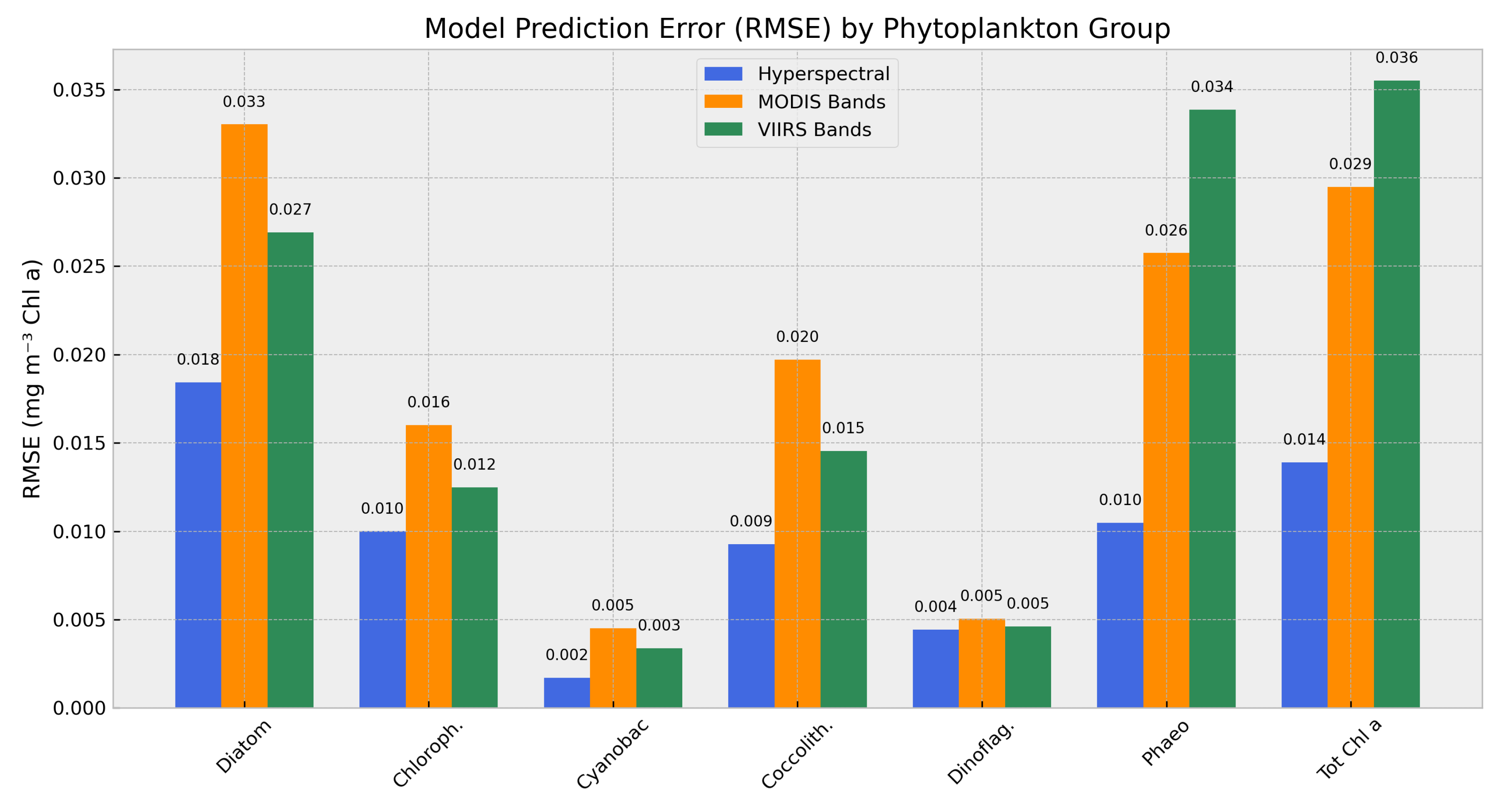
Figure 4.
Predicted vs. true phytoplankton concentrations using the MODIS-band subset. A dashed 1:1 line indicates perfect prediction. Wider spread around the diagonal reflects increased prediction error due to reduced spectral input.
Figure 4.
Predicted vs. true phytoplankton concentrations using the MODIS-band subset. A dashed 1:1 line indicates perfect prediction. Wider spread around the diagonal reflects increased prediction error due to reduced spectral input.
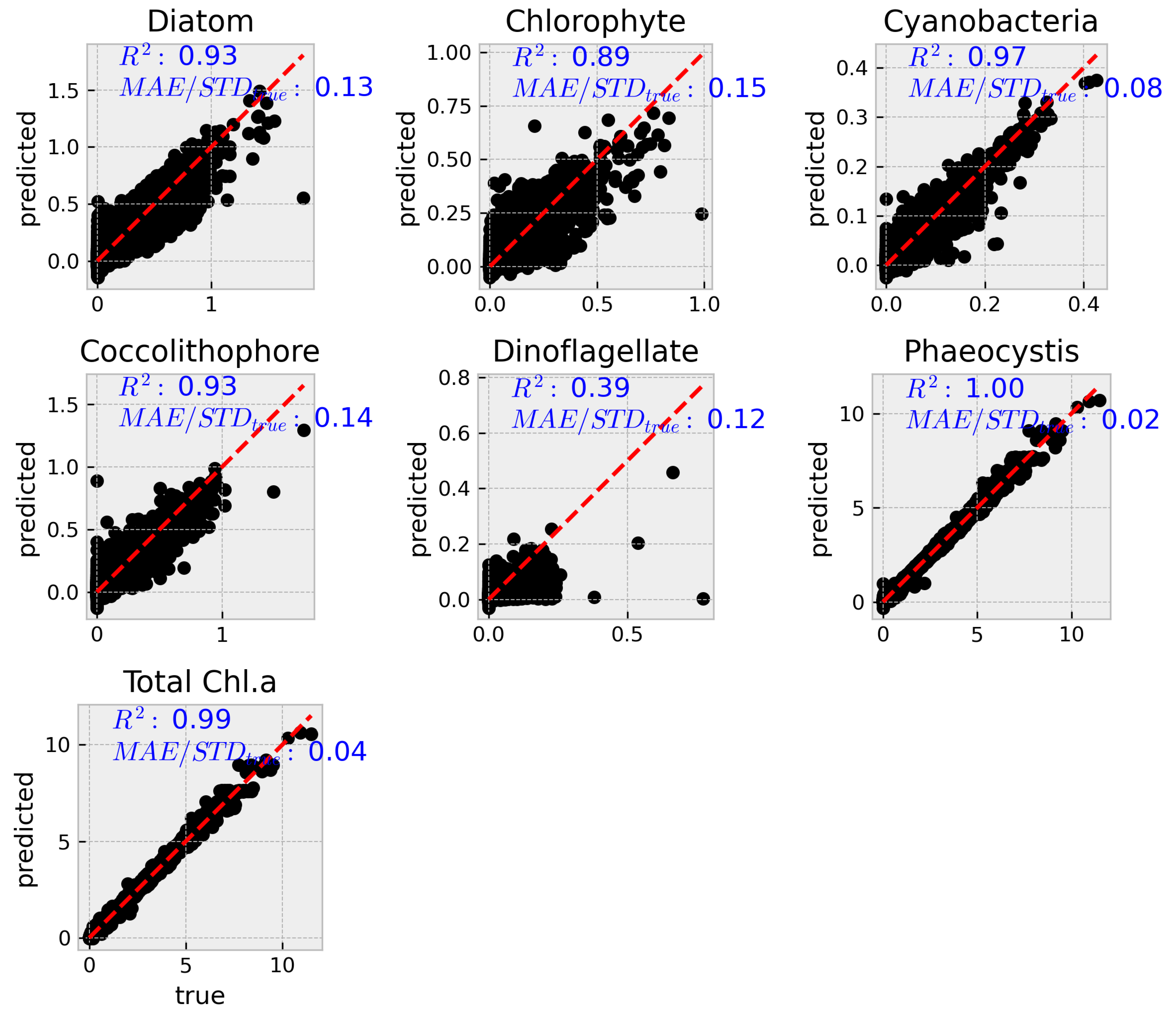
Figure 5.
Predicted vs. true phytoplankton concentrations using the VIIRS-band subset. Despite limited input features, the model maintains good predictive performance across most groups, particularly compared to the MODIS configuration.
Figure 5.
Predicted vs. true phytoplankton concentrations using the VIIRS-band subset. Despite limited input features, the model maintains good predictive performance across most groups, particularly compared to the MODIS configuration.
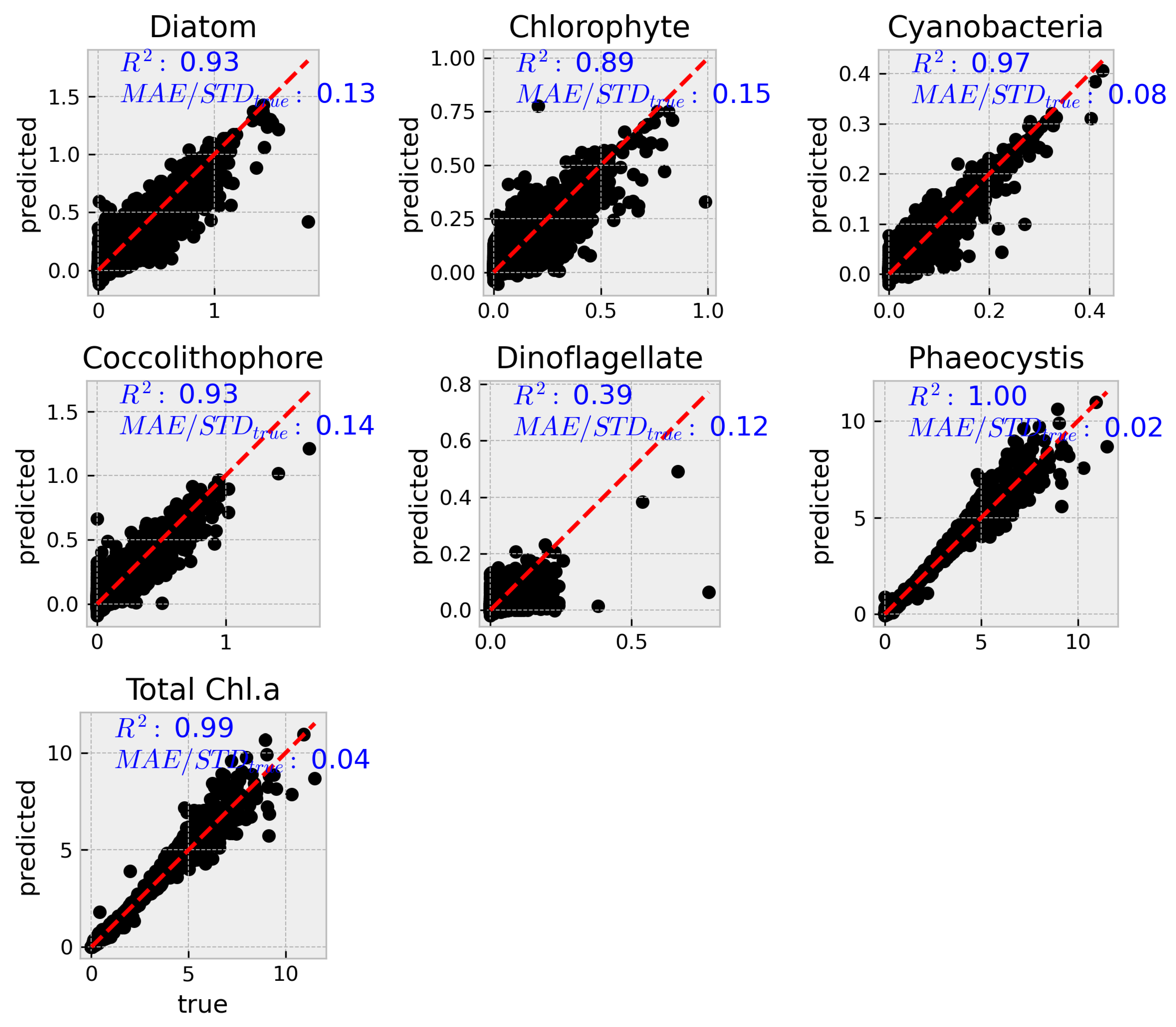

Table 1.
Hyperparameter ranges and their corresponding sampling strategy used in optimization.
| Hyperparameter | Low bound | High bound | Sampling Distribution |
|---|---|---|---|
| Learning rate | Log Uniform | ||
| Max. tree depth | 3 | 10 | Uniform Integer |
| Estimator number | 50 | 500 | Uniform Integer |
| Row sample fraction | Uniform Float | ||
| Column sample frac. | Uniform Float | ||
| Gamma | Log Uniform |
Table 2.
Performance metrics of optimized and trained model on hold-out set.
| Metric | Diatom | Chloroph. | Cyanoac | Coccolith. | Dinoflag. | Phaeo | Tot. Chl_a |
| MSE | 0.00034 | 0.00010 | 2.89e-06 | 8.59e-05 | 1.96e-05 | 0.00011 | 0.000193 |
| RMSE | 0.0184 | 0.0100 | 0.0017 | 0.00927 | 0.00443 | 0.0105 | 0.0139 |
| MAE | 0.00878 | 0.0042 | 0.00078 | 0.0042 | 0.000637 | 0.00313 | 0.00728 |
| R-squared | 0.979 | 0.958 | 0.996 | 0.985 | 0.530 | 0.999 | 0.999 |
| MAE/StDev | 0.0691 | 0.0858 | 0.0302 | 0.0563 | 0.0986 | 0.00754 | 0.0182 |
Disclaimer/Publisher’s Note: The statements, opinions and data contained in all publications are solely those of the individual author(s) and contributor(s) and not of MDPI and/or the editor(s). MDPI and/or the editor(s) disclaim responsibility for any injury to people or property resulting from any ideas, methods, instructions or products referred to in the content. |
© 2025 by the authors. Licensee MDPI, Basel, Switzerland. This article is an open access article distributed under the terms and conditions of the Creative Commons Attribution (CC BY) license (http://creativecommons.org/licenses/by/4.0/).
Copyright: This open access article is published under a Creative Commons CC BY 4.0 license, which permit the free download, distribution, and reuse, provided that the author and preprint are cited in any reuse.


