
Submitted:
01 August 2025
Posted:
04 August 2025
You are already at the latest version
Abstract
The stability of a circular vortex is studied in the thermal quasi-geostrophic (TQG) model. Several radial distributions of vorticity and of buoyancy (temperature) are considered for the mean flow. First, the linear stability of these vortices is addressed. The linear problem is solved exactly for a simple flow and two stability criteria are then derived for general mean flows. Then, the growth rate and most unstable wavenumbers of normal-mode perturbations are computed numerically for Gaussian and cubic exponential vortices, both for elliptical and higher mode perturbations. In TQG, contrary to usual QG, short waves can be linearly unstable on shallow vorticity profiles. Linearly, both stratification and bottom topography (under specific conditions) have a stabilizing role. Second, we use a numerical model of the nonlinear TQG equations. With a Gaussian vortex, we show the growth of small-scale perturbations during the vortex instability, as predicted by the linear analysis. In particular, for an unstable vortex with an elliptical perturbation, the final tripolar vortices can have a turbulent peripheral structure, when the ratio of mean buoyancy to mean velocity is large enough. The frontogenetic tendency indicates how small-scale features detach from the vortex core towards its periphery, and thus feed the turbulent peripheral vorticity. We confirm that stratification and topography are stabilizing as shown by the linear theory. Then, by varying the vortex and perturbation characteristics, we classify the various possible nonlinear regimes. The numerical simulations show that the influence of the growing small-scale perturbations is to weaken the peripheral vortices formed by the instability, and by this, to stabilize the whole vortex. Axisymmetrization replaces tripole formation, and tripole formation replaces dipolar breaking, as the mean buoyancy amplitude is increased. A finite radius of deformation and/or bottom topography also stabilize the vortex as predicted by linear theory. An extension of this work to stratified flows is finally recommended.
Keywords:
geophysical fluid dynamics
; vortex stability
; TQG model
; linear stability criterion
; nonlinear regimes
; vorticity fronts
1. Introduction
Vortices are an essential feature of planetary fluid flows. Their stability has often been studied using the rotating shallow water (RSW) model with one or several homogeneous layers (i.e. with a mean vertical stratification) [1,2,3,4,5]. In particular, these studies showed that vortices with horizontally or vertically sheared velocity profiles can be sensitive to barotropic or baroclinic instabilities. In their nonlinear evolution, strongly unstable vortices break into several fragments. Only for weakly unstable vortices does the perturbation stabilize non-linearly, leading to a vortex multipole. Vortex stability has also been studied in the quasi-geostrophic model, a subset of the RSW equations, valid for low frequency dynamics [6,7,8,9]. These studies also showed that very unstable vortices would break irreversibly into dipoles, while weakly unstable vortices could rearrange as rotating multipoles.
However, neither the RSW model nor the usual quasi-geostrophic model, are appropriate in the presence of a mean horizontal stratification. Therefore, an extension of RSW models to horizontally inhomogeneous layers was derived by [10]. This model was called ILPE (Inhomogeneous Layer Primitive Equation model) — or TRSW (Thermal Rotating Shallow-Water model) for the specific case of the model — in subsequent papers. In his 1993 paper, P. Ripa showed that the pseudo-energy or the pseudo-momentum of flow could not be ascertained to be sign-definite for general flows and therefore that no general criterion for formal stability could be obtained in the ILPE model. This in no way restricts the usefulness of the ILPE nor of the TRSW model. Indeed, they were used to model the upper ocean dynamics [11,12,13] and they were also developed to include moisture for application to the atmosphere [14,15].
The TRSW model equations being difficult to handle, several authors derived a low-Rossby number (low-frequency) version of these equations, called TQG (Thermal Quasi-Geostrophy). Firstly, P. Ripa derived a low-frequency approximation of the ILPE model that he called ILQG [16]. The equations of this model are those later called thermal quasi-geostrophic (TQG) equations, also derived and studied by [17] and by [18]. A numerical analysis of the TQG equations was achieved by [19]. [20] derived a criterion for the nonlinear saturation of thermal instabilities in this model.
[21] studied numerically the stability of jets and vortices in the TRSW model and showed that small-scale features appear as the instability develops. The complexity of the TRSW model renders difficult any analytical work on jet or vortex stability. Therefore, we use the TQG model here, to analyze the instability of circular vortices. After recalling the model equations (Section 2), we provide analytical solutions for linear stability in a vortex core, and then a general stability criterion for circular flows (Section 3). We also compute the growth rates and unstable waves for several velocity and buoyancy distributions numerically. In Section 4, we use a numerical model to classify the nonlinear regimes of thermally unstable vortices in the TQG dynamics. We analyze the finite-time evolution of these vortices with a Fourier analysis and the frontogenesis function. Finally, we conclude this study.
2. Model
2.1. Equations
We mostly follow the notations introduced by [19] to express the two equations of the Thermal Quasi-Geostrophic model as:
where
is the potential vorticity, is the streamfunction, is the deformation radius (taken as unity by [19]). In these notations, g is gravity, H is the maximal thickness of the fluid layer at rest, and f is the Coriolis parameter, chosen constant here. In these equations, b is the buoyancy (which depends directly on temperature via the equation of state of the fluid, assuming no other active tracer). All variables depend only on the horizontal coordinates, being vertically averaged.
In the equations above, the velocities are given by the following relations
where is the bottom height above the maximal depth and the vertical unit vector.
2.2. Flow and buoyancy distributions
As we study vortices here, the mean velocity and buoyancy distributions will be chosen circular, and thus dependent on the radius r only, .
In particular, to derive simple analytical solutions in SubSection 3.1, we will use
which is an acceptable form for the core of oceanic vortices, see for instance [22,23]. We define the tangential velocity of the mean flow (its radial component is null), and the corresponding mean rotation rate. Bottom topography will be included only locally in this study.
For the derivation of the linear instability criterion (in SubSection 3.2 and Section 3.3), a general form of these functions will be kept. Finally, for the numerical study of both linear and nonlinear evolutions of unstable vortices (SubSection 3.4 and Section 4), Gaussian or power-exponential profiles of mean streamfunction and buoyancy will be considered.
Power exponential vortices have the following profile of vorticity and of buoyancy
with , being the vortex azimuthal velocity and its radius. is the vortex buoyancy.
For the linear instability analysis, angular normal modes will be used
where l is the angular mode (or azimuthal mode), and the complex value of contains the phase speed of the perturbation (the real part of c) and the growth rate of the perturbation (). With such perturbations, the linearized equations of vorticity and of buoyancy are
in the absence of bottom topography ().
2.3. Linear and nonlinear numerical models
In SubSection 3.4, when using normal mode perturbations and when discretizing the radius over N grid points (), the linear equations 8, become a matrix system, in and b. This system is solved by diagonalization, c being the eigenvalue and being the corresponding eigenvector. We thus obtain , where the A and B matrices depend on .
In Section 4, the numerical simulations with the system of nonlinear equations 1, will be carried out with a pseudo-spectral code of these equations, on a bi-periodic horizontal grid. The number of grid points is 512 horizontally. The code uses a mixed Euler-leapfrog scheme in time which is conservative in vorticity and buoyancy, and which does not separate odd and even solutions in time-steps. The horizontal derivatives are performed in spectral space, using fast Fourier transforms to recover physical variables. Very weak bi-harmonic viscosity is added to equations 1, which does not alter the physical results (tests have been performed with different small values of viscosity).
3. Linear stability
3.1. A simple analytical solution
Firstly, we look for an analytical solution to equations 8, ; this is possible only for simple mean streamfunction and buoyancy profiles. Here we choose such profiles, which are realistic for the core of vortices. It is not possible to solve analytically the problem for the whole vortex, but in the core resides most of the mean kinetic (or potential) energy which feeds the perturbation.
The mean potential vorticity is and therefore
With this, the linear equations are
The last step relates and . This is achieved by considering eigen-functions of the Laplacian operator in polar coordinates
which leads to (for simplicity, we have not specified here that we take the real part of the expression above; therefore is complex).
Similarly, we set
This provides a homogeneous system in whose determinant must vanish. This determinant is
Instability will occur in such a vortex core if
Thus, a necessary condition for instability in this case is .
We can analyze condition more fully. Setting , this condition can also be written as . Some short algebra indicates that this is possible only if and .
When adding topography to the problem, we can choose a parabolic seamount , so that . Then we have a new condition for instability
Since , a seamount stabilizes the flow if , and conversely.
3.2. Stability criterion
After this first simple solution, we look for a general stability criterion for TQG vortices. Now we do not choose a specific form of , nor of any more. Equation 8 could be amenable to a Rayleigh-type criterion by multiplying it by (the complex conjugate of ), but then the coupled term in should be eliminated; this implies to multiply equation by the proper quantity for a further substitution. This is done in SubSection 3.3. Here we choose to express in terms of using equation , without multiplying equations 8, by complex conjugates of or immediately.
This equation resembles the Taylor-Goldstein equation. This can be understood since they both result from a vorticity and a buoyancy equation (in different planes, horizontal or vertical). Thus, it is appropriate to use the change of variable . Setting , some algebra leads to the equation
where is the derivative of .
Only now do we multiply this expression by which is the complex conjugate of and we integrate the equation over r as . This leads to
We can take the imaginary part of this expression; the central term will vanish and we will be left with
For to be non-zero, the second integral must be positive. Therefore, we must have
at some r, for instability; this is a necessary condition.
We can also write this inequality as
Applying this inequality to the case of SubSection 3.1, we obtain , for instability, which is the condition previously found.
We can generalize this criterion to the presence of bottom topography . Defining , we need to have
at some r, for instability. Again, we can see that a seamount is stabilizing for positive .
3.3. A second instability criterion
As mentioned in the previous subsection, we can multiply equation 8 by , the complex conjugate of and divide it by , leading to
we also multiply the complex conjugate of equation by and divide it by , leading to
Finally, we eliminate between these two equations, and integrate to obtain
where
are (twice) the kinetic, potential energies of the perturbation.
Let us now take the imaginary part of this equation; it is
For the vortex to be unstable, must be non-zero (positive), and therefore the two terms in the integral must be opposite-signed. Thus, a necessary condition for instability is
Since this criterion involves , it is less straightforward to apply.
We have not found how to substitute by some rigorously, as in the Fjortoft criterion. Obtaining exactly requires solving the linear instability problem (numerically), which is not possible for all mean flow and buoyancy distributions. A rough estimate of could be computed from our analytical solution at marginality.
3.4. Numerical analysis of linear stability
Now we choose a realistic mean distribution of to discretize equations 8, over the N steps in r and to solve the linear instability problem numerically. We start with Gaussian mean distributions of streamfunction and of buoyancy
For simplicity, we set . This provides a length and a time scale. We also set unless otherwise stated.
As a reference, we solve equations 8, with ; this is the 2D incompressible flow case that is well known [24,25]). For the TQG case, we set .
Figure 1a shows the growth rate versus the azimuthal wavenumber l for both cases. In the 2D flow, only is unstable for Gaussian vortices. In the TQG flow, the Gaussian vortex is linearly unstable for all wavenumbers from to . In TQG, there is no universally stable solution for , contrary to 2D [24]. Furthermore, all growth rates are much larger in TQG than in 2D (twice as large for ). From this, we can conclude that TQG vortices are not only more unstable than their 2D counterparts, but also that they will develop smaller-scale perturbations. The origin of these differences between the two models can be searched in equations 8, . Firstly, it is clear that if we set in both equations, then , and equation 8 becomes the 2D linear equation. Therefore, a non-zero mean buoyancy gradient is necessary to account for this difference. It is also of interest to see that if we cancel the mean buoyancy gradient in the second equation only, the growth rates in this case are comparable to those of 2D as long as . In this case, like-signed and increase the mean vorticity/buoyancy gradient. More interesting is the cancellation of the term only, in equation 8; this renders the first equation 2D-like (independent from ); equation then only provides as a function of and the growth rates are those of 2D, again in the limit . Therefore, clearly, the term is responsible for the difference between the two dynamics, TQG on the one hand, and 2D with a passive b tracer, on the other hand.
For the same (Gaussian) flow, we study now the influence of the ratio on the growth rate for (see Figure 1b). Clearly, in the TQG model, the coupling of the vorticity equation with the buoyancy equation destabilizes the flow for small values of this ratio (compared to the 2D model). Increasing this ratio to unity then decreases the growth rates. A maximal growth rate is obtained for .
Again for the Gaussian vortex, with and with , we test the sensitivity of growth rates to free surface effects. We call and plot on Figure 1c, the growth rates with respect to both in 2D and in TQG. In TQG, the growth rates of horizontal shear instability decrease when increases, as in 2D flows [26].
Finally, still for the Gaussian vortex, with and with , we test the sensitivity of growth rates to bottom topography. This bottom topography is chosen via (see its formal expression in SubSection 3.2). Figure 1d confirms that a seamount stabilizes the flow if .
In 2D flows, it is well known that the growth rates of the perturbation increase with the mean vorticity shear of the vortex. To this aim, we now use the following family of profiles, also known as -exponential profiles [27], for the velocity
Figure 2a shows the growth rates versus in the 2D case (), and Figure 2b in the TQG case.
As usual for 2D dynamics, we observe that increases with for ; is not large enough in the chosen range to allow the growth of modes . We recover the critical value of for as mentioned in [27]. Barotropic instability occurs only for steep enough vortices, all the more so as the waves are short.
On the contrary, in TQG dynamics, vortices with "flat" vorticity profiles are unstable to both long and short waves. A small growth rate exists for over a wide range of values of . The curves for emerge from this minimal growth rate; it must be noted that for large enough (), the growth rates in the 2D and TQG are comparable for .
Physically, one must exert caution for , though the results are mathematically correct. For , we have . Vorticity behaves as near the center and, in a two-dimensional representation, exhibits a cusp at the center. Therefore, it is recommended to consider only cases with .
4. Nonlinear evolution
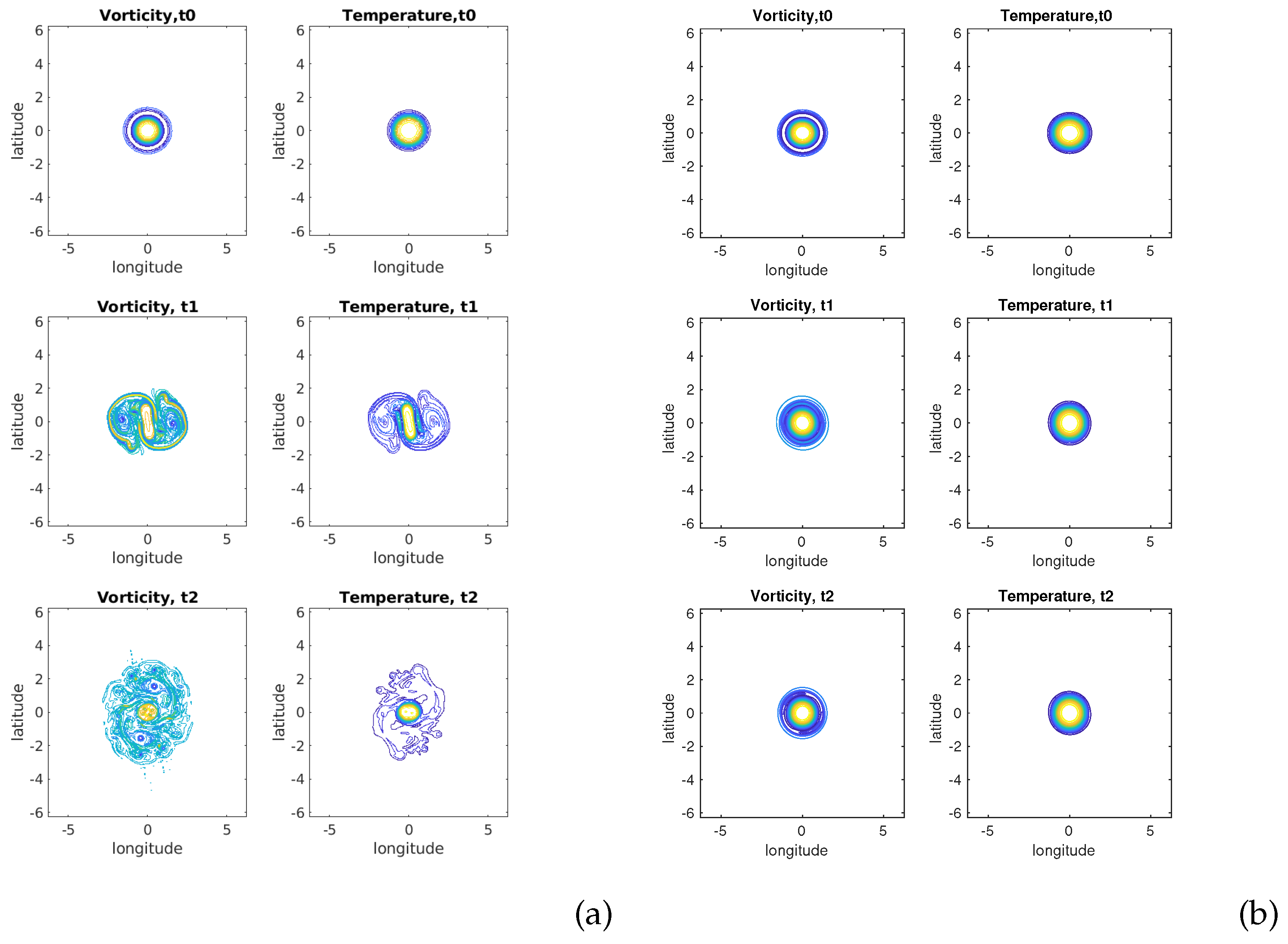
After the linear analysis of stability, we study numerically the nonlinear regimes of perturbed unstable vortices. Firstly, we study a reference case with Gaussian distributions of buoyancy and streamfunction, with a given ratio between their amplitude, and an elliptical perturbation. Then we will vary all these parameters, and briefly study the influence of a finite deformation radius and of circular topography.
4.1. Reference case
Our reference case has
with only an elliptical perturbation initially (Figure 3a-b at time ). With these conditions, we ran the TQG model and the decoupled 2D model in parallel. Figure 3 shows the time evolution of vorticity and of buoyancy in the two cases. Initially, the decoupled 2D model dynamics creates filaments during the reorganization of the vortex periphery, yet fewer than the TQG model (see fig.3a-b at time ). At finite times, the TQG model creates many small scale features than the decoupled model, in particular radially. This is not the case of the 2D decoupled model (same figures at time ).
To interpret this appearance of fronts, we note again that the term plays a key role in the coupling of the vorticity and buoyancy equations. Vorticity and thermal Rossby waves propagate circularly on the radial vorticity and buoyancy gradients. Since these gradients (and the mean flow) are not constant, the buoyancy anomaly of these waves is sheared and forms filaments, Via the coupling, vorticity anomalies are formed; they are also sheared. This is clearly seen in the TQG model vorticity plots (Figure 3a). The buoyancy distribution being more spread out that that of vorticity, filaments are formed mostly around the vortex core. The vorticity anomalies lead to shear flow growth, which increase and .
To quantify this process further, we decompose the vorticity anomalies azimuthally in Fourier modes, and radially in Bessel components. This is done via
where R is an arbitrary radius (here chosen as ), large enough to encompass the vortex core and periphery. The modal amplitudes are plotted on Figure 4a,c. For sake of clarity l was considered continuous on the graph, but only the integer values of l have to be considered. Clearly, mode remains the dominant (and nearly sole) mode in the decoupled evolution, while higher modes are much stronger in the TQG model. They correspond, in physical space, to the small-scale features observed in the vorticity field.
Secondly, for , we project and onto a basis of Bessel functions using their orthogonality.
and
where is the vortex radius (here equal to unity), and is the root of the Bessel function . It is known that for increasing , the Bessel function oscillates faster radially (corresponding to thinner structures). For sake of clarity k was considered continuous on the graph, but only the integer values of k have to be considered. Figure 4b,d indicate that radially short perturbations (components ) grow initially on the vortex in the decoupled 2D dynamics, but they rapidly decay afterwards. On the contrary, short radial perturbations remain of larger amplitude in the TQG dynamics for the whole duration of the simulation.
Now, we compute the two components of the deformation, the normal strain rate , the shear strain rate and, from them, the total strain rate . We plot this latter, for in the simulation, on Figure 5a,b for the TQG and the decoupled models. Clearly, the deformation rate is stronger and more spread out in the TQG simulation. Also many more small-scale intricate patterns are seen in this simulation compared with the 2D decoupled model one.
Finally, using the Lagrangian conservation of buoyancy in both TQG and 2D equations, one can derive an equation for the evolution of the gradient of buoyancy (equivalently, of buoyancy)
which can be multiplied by the adjoint of the buoyancy gradient to yield
The frontogenetic tendency, or frontogenesis function, F indicates where the buoyancy (or buoyancy) gradients will amplify or decay, and thus where filaments will grow or disappear. This function is shown for our TQG simulation on Figure 6. The regions shown correspond to the regions of strong buoyancy gradient in Figure 3a at . Clearly, buoyancy gradients are formed in the vicinity of the deformed vortex core; they tend to disappear in the periphery.
4.2. Parameter sensitivity
4.2.1. Vorticity profile steepness and relative intensity of the mean buoyancy
Firstly, for an elliptical perturbation (), we vary the steepness () of the mean velocity and buoyancy profiles and the ratio of their intensities (). Here we have
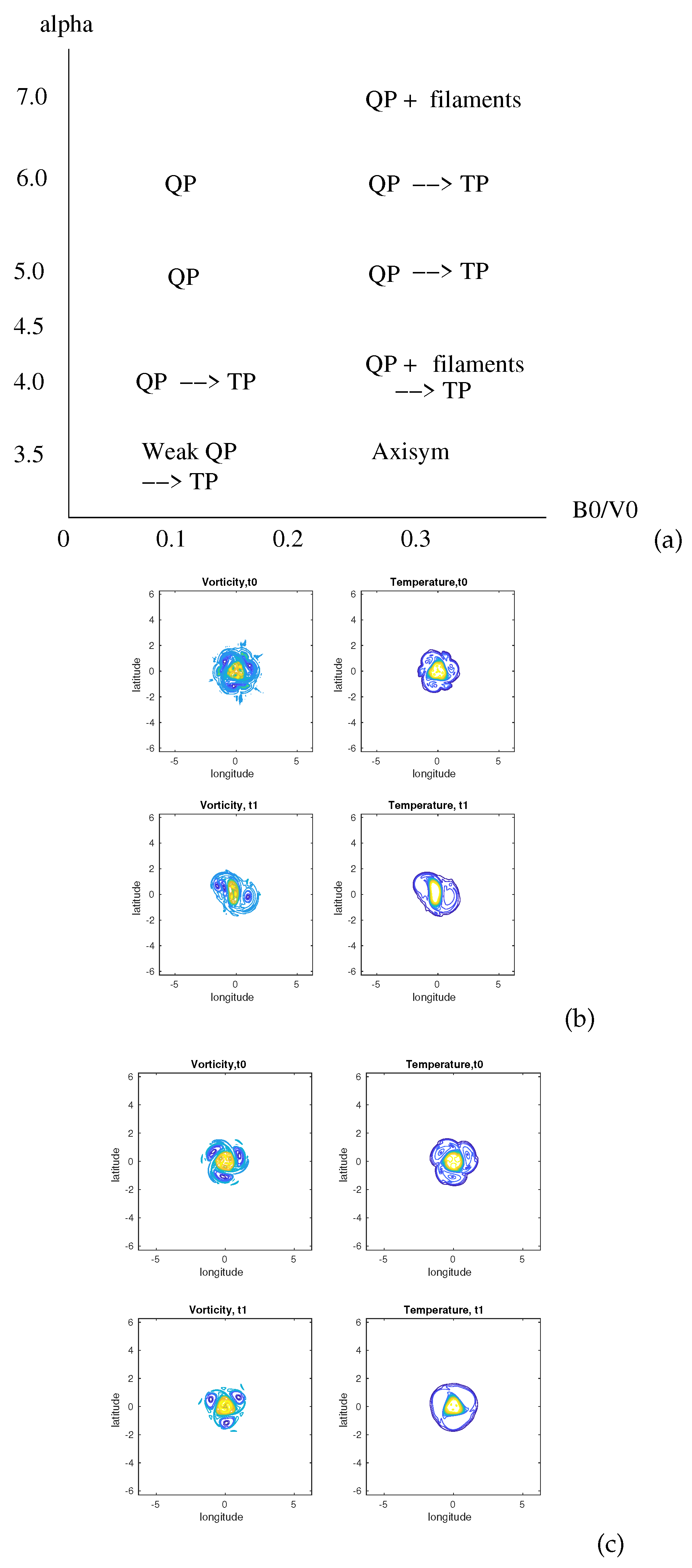
Figure 7a indicates that for Gaussian vortices (), tripoles are formed by the instability of the circular vortex. Tripole formation is all the less efficient as grows. For large values of this ratio, the end-state of the nonlinear simulation is a quasi-axisymmetric vortex. Indeed, as mean buoyancy is larger, the vortex is more prone to small-scale instabilities (as was shown by linear instability theory). This renders the satellites of the tripole less coherent. Thus, their robustness is lesser and the shear that they exert on the vortex core is weaker. For large , the satellites are not coherent any more and the tripolar state is only transient.
For steeper vortices, the present of filaments in the tripole satellites and around them becomes more prevalent until the whole vortex periphery is completely turbulent (for growing , with constant ; see Figure 7b). Also a mode is observed in the vortex evolution, due both to wave-wave interaction (from the fundamental mode ) and to the growth of small waves in the TQG model (see also Figure 7b). For steep vortices, the radial gradient of mean vorticity is large enough to lead to vortex breaking into two dipoles (the usual irreversible, fully nonlinear, evolution of strongly unstable vortices with see Figure 7c). Then, nonlinear harmonic formation from is more efficient than the growth of small waves via the TQG dynamics. Again, for large , the tripole satellites lose their coherence and are not able to maintain large enough a shear on the vortex core and the whole structure tends towards axisymmetry.
4.2.2. Influence of stratification and of bottom topography
To assess the influence of stratification, we run simulations of the case , increasing from zero. We have run the model with three values of : 0.25, 1.0, 4.0.
Figure 8 shows the various final states of vorticity and buoyancy (with increasing from left to right). Clearly, the vorticity satellites (in the periphery), contributing to the tripolar shape of the vortex, and the small-scale features are progressively erased by the increasing vortex stretching. The vortex core is also more circular. This confirms the linear stability analysis which indicated a decreasing instability with increasing .
To assess the role of bottom topography, we run a simulation with a cubic exponential vortex (, with , , an elliptical perturbation () and a Gaussian topography , with . In Figure 8, we compare the nonlinear evolution of a quartic exponential vortex () perturbed elliptically () with , over flat bottom (no topography) and over a seamount (positive topography). Over the flat bottom, the unstable vortex transforms first into a tripole with filamentary satellite, an evolution already seen (above). Finally, the vortex periphery becomes turbulent with many small-scale features. On the contrary, over the seamount the perturbation seems damped and the vortex becomes quasi circular. This stabilization is in agreement with the linear stability analysis.
Figure 9.
End-states of simulations for a quartic exponential vortex () with and ; (a) Vorticity and buoyancy maps at without bottom topography; (b) vorticity and buoyancy maps at over a Gaussian seamount of height and of radius ).
Figure 9.
End-states of simulations for a quartic exponential vortex () with and ; (a) Vorticity and buoyancy maps at without bottom topography; (b) vorticity and buoyancy maps at over a Gaussian seamount of height and of radius ).
4.2.3. Nonlinear evolutions with higher wavenumber perturbations
As shown by [28,29,30], more complex vortex aggregates than tripoles can exist in two-dimensional incompressible flows. Therefore, we study here their possible counterparts in the TQG model. We search quadrupolar vortices formed from the instability of circular vortices, with a mode initial perturbation. The growth of higher wavenumber perturbations on a power-exponential vortex, requires a higher degree of the power (a larger horizontal velocity shear), than that of low-mode perturbations. Here, we consider power-exponential vortices (equation 3) with .
Figure 10a sumarizes the various nonlinear evolutions of the unstable vortices when or . We note that a smaller horizontal shear is needed to stabilize a quadrupole nonlinearly with is small while quadrupoles degenerate into tripoles for larger values of when .
Again this shows that the presence of buoyancy in the mean flow weakens the ability of the initial perturbation to grow and (possibly) stabilize nonlinearly at large amplitude. For this larger value of the mode is less prevalent. It either decays and the vortex axisymmetrizes or it gives way to an elliptical (asymmetric) disturbance.
We also note that for large more filaments (short-scale perturbations) develop.
5. Discussion
Our study has, first, provided stability criteria and simple solutions to understand the effect of buoyancy coupling with vorticity, on the instability of circular vortices. They have shown that the vortices are then more unstable than in a 2D model, with notably larger growth rates for short waves. Second, and paradoxically, the numerical simulations have shown that, if the short waves indeed grew more in a TQG model, they have a rather stabilizing effect on the nonlinear evolution of the linearly unstable vortices, compared with the 2D case. This is explained as follows:
During the development of the instability of these vortices, the external annulus of vorticity breaks into l independent vortices. These peripheral vortices can deform and break the vortex core, leading either to rotating multipoles, or to l dipoles. But, in the TQG model, the appearance of filaments and of small vortices render these peripheral vortices less coherent. As a consequence, these latter exert a weaker shear on the vortex core and do not distort it as much. Thus the vortex is finally less unstable in the nonlinear evolution.
Note that these results do not depend on our explicit choice of alpha-exponential vortices for the mean circular flow; this choice is usual in view of observations of vortices at sea [9]. But previous studies [24] have shown that the analytical form of this radial profile of vorticity is not essential, as long as it belongs to a family of vortices (e.g. unshielded monopoles, monopoles, unshielded annuli, etc.).
Now, only barotropic (horizontal shear) instability has been studied here and it would be of interest to generalize our results to at least a two-layer TQG model to allow the study of baroclinic instability. Note that the TQG equations are not fully coupled (vorticity is not included in the buoyancy equation), contrary to the two-layer quasi-geostrophic (QG) equations in which each layerwise potential vorticity depends on the other layer streamfunction. Therefore, we can expect new coupling mechanisms between vorticity and buoyancy in a two-layer model.
Also, concerning the equations, the vorticity and buoyancy equations are different in mathematical structure (even if they were not coupled): buoyancy is directly advected while streamfunction is modified via vorticity advection followed by inversion; the inversion of the Laplacian has a widening effect on horizontal fields. This is another difference between the two-equation TQG model and the two-equation two-layer QG model.
Continuing with the analogy and differences between TQG and QG models, we must note that TQG dynamics share with SQG (surface quasi-geostrophy, [31]) the ability to generate small-scale features in the nonlinear dynamics. But a major dynamical difference exists in these two models. In the TQG model, the streamfunction derives from the inversion of the vorticity. Therefore, the external velocity field of a vortex decays as . In the SQG model, the streamfunction is obtained from the inversion of the buoyancy (a square root of the Laplacian of streamfunction). This leads to a different Green’s function for the inversion and the external velocity field of a buoyancy patch (in SQG) decays in . Therefore, the small-scale features are dynamically less active in the SQG than in the TQG model. Consequently, vortex instability in the SQG model has much similarity with that in the 2D model, contrary to TQG.
One can add that even in the shallow-water (SW) model, where velocity is not geostrophic, vortex instability is comparable to that observed in QG. Therefore, TQG stands apart in this whole range of models (2D, QG, SQG, SW, TQG). It must be remembered that it is an idealized and simplified model. Comparison with oceanic features is difficult, all the more so as the specificity of TQG is the formation of small-scale features, not easily observed via in situ nor satellite sensors.
6. Conclusions
The previous study of vortices in the thermal rotating shallow-water (TRSW) model [21] has yielded features and evolutions quite comparable to those observed in our study. A detailed comparison between TQG and TRSW is now desirable to assess the role of non-geostrophic velocity in vortex evolution in these models. Can our stability criteria be extended, for instance, to weakly non-geostrophic flows ?
For oceanographic applications, it could be of interest to compare vortex dynamics in the TQG model to those in a primitive-equation model with a surface mixed layer. Indeed, such a model would include all physical processes at work in the ocean: in particular low and high frequency dynamics (the latter being excluded in TQG), mechanical and thermohaline forcing by the atmosphere, complete thermodynamics, etc. Realistic ocean models could serve more easily a testbed for TQG than oceanographic observations (for the reasons mentioned above). A next step in the assessment of TQG models could be the coupling of two such models, one for the ocean surface and one for the atmospheric boundary layer, and the study of vortex and jet dynamics in such coupled models. This research is underway.
Author Contributions
“Conceptualization, X.C.,Y.B.,G.R.; methodology, X.C.; software, X.C.; validation, X.C.,Y.B.,G.R.; formal analysis, X.C., Y.B.; writing—original draft preparation, X.C., Y.B.,G.R.. All authors have read and agreed to the published version of the manuscript.”.
References
- Ripa, P. General stability conditions for a multi-layer model. Journal of Fluid Mechanics 1991, 222, 119–137. [Google Scholar]
- Dewar, W.K.; Killworth, P.D. On the Stability of Oceanic Rings. Journal of Physical Oceanography 1995, 25, 1467–1487. [Google Scholar]
- Killworth, P.D.; Blundell, J.R.; Dewar, W.K. Primitive Equation Instability of Wide Oceanic Rings. Part I: Linear Theory. Journal of Physical Oceanography 1997, 27, 941–962. [Google Scholar]
- Dewar, W.K.; Killworth, P.D.; Blundell, J.R. Primitive-Equation Instability of Wide Oceanic Rings. Part II: Numerical Studies of Ring Stability. Journal of Physical Oceanography 1999, 29, 1744–1758. [Google Scholar]
- Baey, J.M.; Carton, X. Vortex multipoles in two-layer rotating shallow-water flows. J. Fluid Mech.
- Drtischel, D.G.; Scott, R.K.; Reinaud, J.N. The stability of quasi-geostrophic ellipsoidal vortices. Journal of Fluid Mechanics 2005, 536, 401–421. [Google Scholar]
- Reinaud, J.N.; Carton, X. The stability and the nonlinear evolution of quasi-geostrophic hetons. Journal of Fluid Mechanics 2009, 636, 109–135. [Google Scholar]
- Reinaud, J.N. Three-dimensional quasi-geostrophic vortex equilibria with m-fold symmetry. Journal of Fluid Mechanics 2019, 863, 32–59. [Google Scholar]
- Carton, X.; Sokolovskiy, M.; Ménesguen, C.; Aguiar, A.; Meunier, T. Vortex stability in a multi-layer quasi-geostrophic model: application to Mediterranean Water eddies. Fluid Dynamics Research 2014, 46, 061401. [Google Scholar]
- Ripa, P. Conservation laws for primitive equations models with inhomogeneous layers. Geophysical & Astrophysical Fluid Dynamics 1993, 70, 85–111. [Google Scholar]
- Lavoie, R. A mesoscale numerical model of lake-effect storms. Journal of the Atmospheric Sciences 1972, 29, 1025–1040. [Google Scholar]
- O’Brien, J.; Reid, R. The non-linear response of a two-layer, baroclinic ocean, to a stationary axially-symmetric hurricane. Part I. Upwelling induced by momentum transfer. Journal of the Atmospheric Sciences 1967, 24, 197–207. [Google Scholar]
- McCreary, J.; Kundu, P.; Molinari, R. A Numerical Investigation of Dynamics, Thermodynamics and Mixed-Layer Processes in the Indian Ocean. Progress in Oceanography 1993, 31, 181–244. [Google Scholar]
- A. Kurganov, Y.L.; Zeitlin, V. Moist-convective thermal rotating shallow-water model. Physics of Fluids 2020, 32, 066601. [Google Scholar]
- A. Kurganov, Y.L.; Zeitlin, V. Interaction of tropical cyclone-like vortices with sea-surface temperature anomalies and topography in a simple shallow-water atmospheric model. Physics of Fluids 2021, 33, 106606. [Google Scholar]
- Ripa, P. Low frequency approximation of a vertically averaged ocean model with thermodynamics. Revista Mexicana de Fisica 1996, 42, 117–135. [Google Scholar]
- Warneford, E.S.; Dellar, P.J. The quasi-geostrophic theory of thermal shallow-water equations. Journal of Fluid Mechanics 2013, 723, 374–403. [Google Scholar]
- Wang, X.; Xu, X. The QG limit of the rotation thermal shallow water equations. Journal of Differential Equations 2024, 401, 1–29. [Google Scholar]
- Wang, X.; Xu, X. Theoretical and computational analysis of the thermal quasi-geostrophic model. Journal of Nonlinear Science, :96.
- Beron-Vera, F.J. Nonlinear saturation of thermal instabilities. Physics of Fluids 2021, 33, 036608. [Google Scholar]
- Wang, X.; Xu, X. Thermal instability in rotating shallow-water with horizontal temperature/density gradients. Physics of fluids 2017, 29, 101702. [Google Scholar]
- Paillet, J.; Le Cann, B.; Serpette, A.; Morel, Y.; Carton, X. Real-time tracking of a Galician Meddy. Geophysical Research Letters 1999, 26, 1877–1880. [Google Scholar]
- Paillet, J.; Cann, B.L.; Carton, X.; Morel, Y.; Serpette, A. Dynamics and Evolution of a Northern Meddy. Journal of Physical Oceanography 2002, 32, 55–79. [Google Scholar]
- Gent, P.R.; McWilliams, J.C. The instability of barotropic circular vortices. Geophysical and Astrophysical Fluid Dynamics 1986, 35, 209–233. [Google Scholar]
- Carton, X.; McWilliams, J.C. Barotropic and Baroclinic Instabilities of Axisymmetric Vortices in a Quasigeostrophic Model. Elsevier oceanography series 1989, 50, 225–244. [Google Scholar]
- Carton, X.J.; McWilliams, J.C. Nonlinear oscillatory evolution of a baroclinically unstable geostrophic vortex. Dyn. Atmos. Oceans.
- Carton, X.J.; Flierl, G.R.; Polvani, L.M. Carton, X.J.; Flierl, G.R.; Polvani, L.M. The generation of tripoles from unstable axisymmetric isolated vortex structures. Europhysics Letters, pp. 339–344.
- Ruben, R. Trieling, GertJan F. van Heijst, v.G.J.F.; Kizner, Z. Laboratory experiments on multipolar vortices in a rotating fluid. Physics of Fluids 2010, 22, 1–12. [Google Scholar]
- Carnevale, G.F.; Kloosterziel, R.C. Emergence and evolution of triangular vortices. Journal of Fluid Mechanics 1994, 259, 305–331. [Google Scholar]
- Kloosterziel, R.C.; Carnevale, G.F. On the evolution and saturation of instabilities of two-dimensional isolated circular vortices. Journal of Fluid Mechanics 1999, 388, 217–257. [Google Scholar]
- Held, I.; PierreHumbert, R.T.; Garner, S.T.; Swanson, K.L. Held, I.; PierreHumbert, R.T.; Garner, S.T.; Swanson, K.L. Surface quasi-geostrophic dynamics. J. Fluid Mech. 1995, pp. 1–20.
Figure 1.
(a) Growth rates versus angular wavenumber l for the Gaussian vortex in the 2D and TQG flows, ; (b) Growth rates versus the ratio for the Gaussian vortex in the TQG flow, ; (c) Growth rates versus for the Gaussian vortex in TQG and in 2D, ; (d) Growth rates versus for the Gaussian vortex in TQG, .
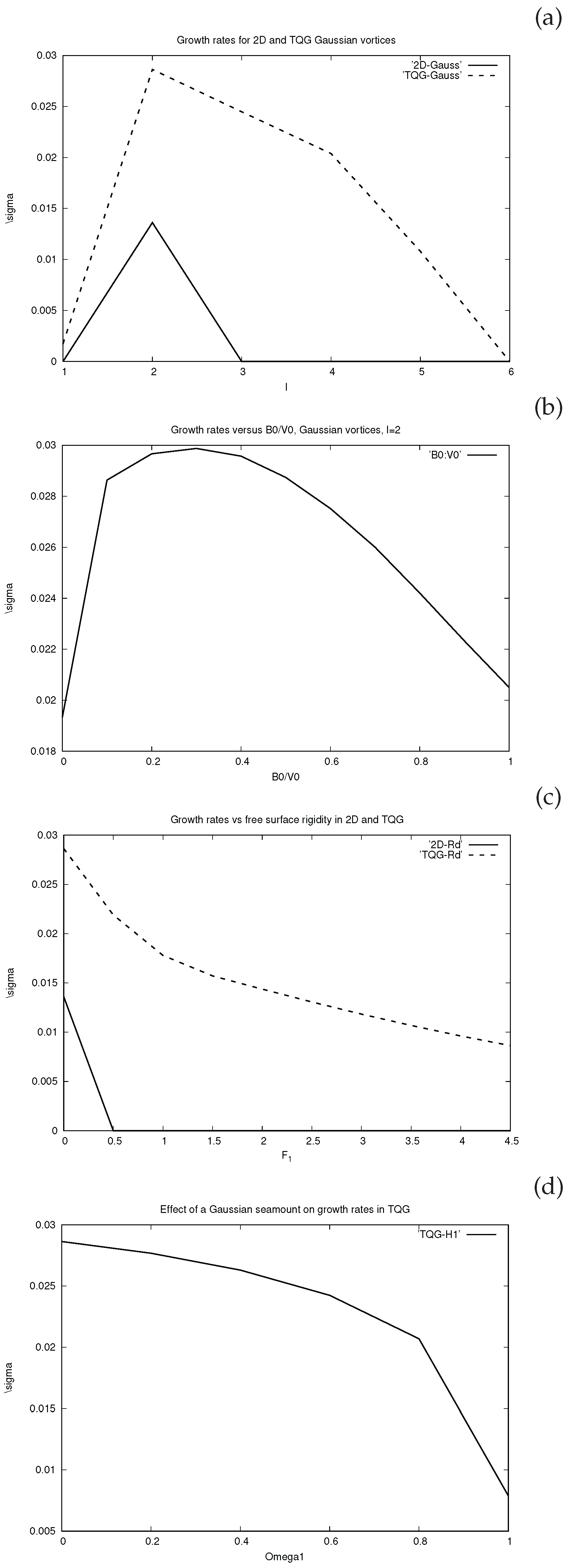
Figure 2.
(a) Growth rates versus in 2D, with ; (b) same for TQG, with .
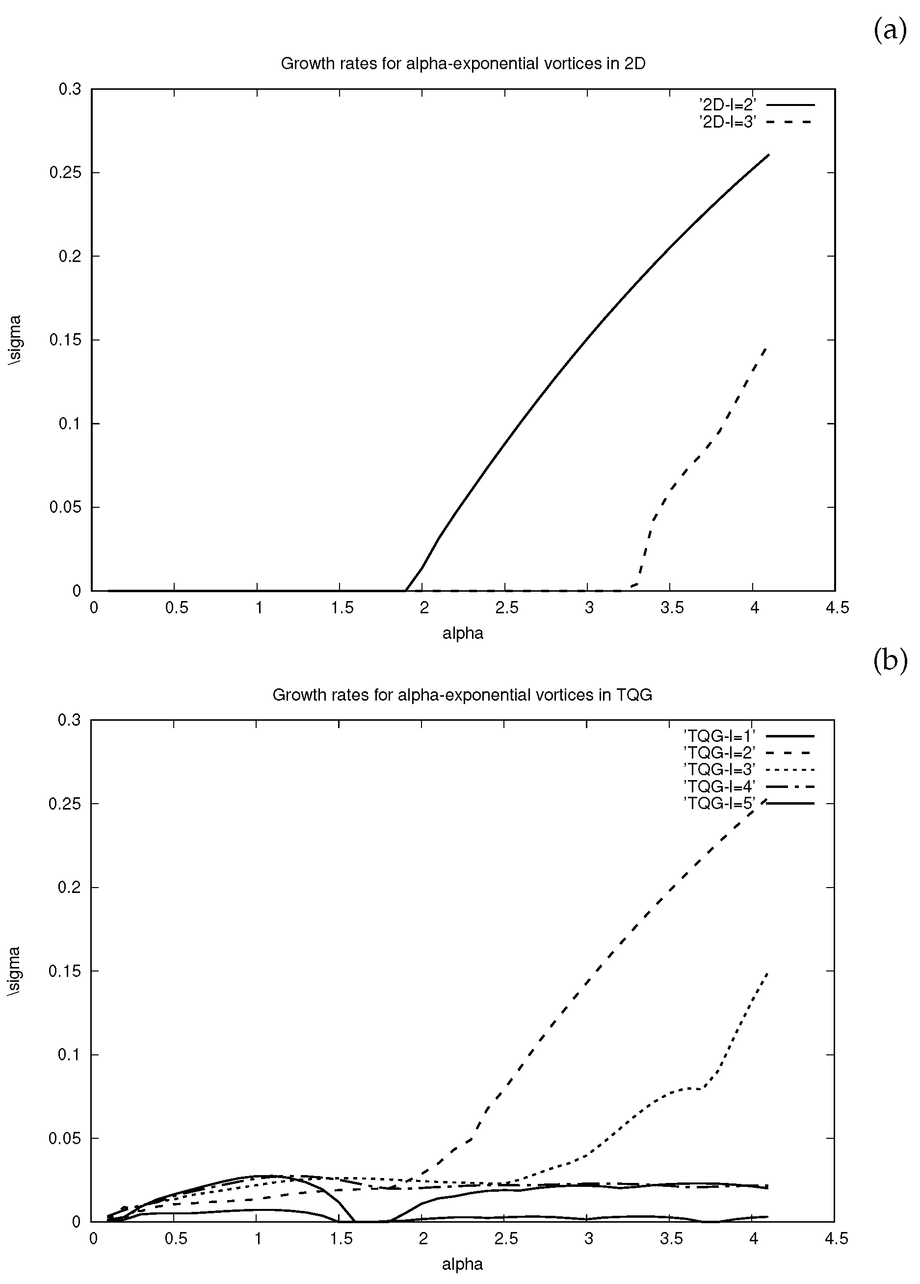
Figure 3.
(a) Time evolution of vorticity (left) and of buoyancy (right) for the TQG simulation with model time units ; (b) same for the decoupled 2D-passive buoyancy model.
Figure 3.
(a) Time evolution of vorticity (left) and of buoyancy (right) for the TQG simulation with model time units ; (b) same for the decoupled 2D-passive buoyancy model.
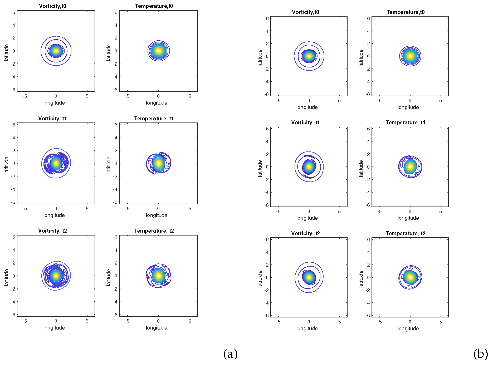
Figure 4.
(a) amplitude of vorticity anomalies with respect to the azimuthal mode l and to time in the TQG model; (b) amplitude of vorticity anomalies with respect to the radial component k and to time in the same model; (c,d) same as (a.b) for the decoupled 2D model
Figure 4.
(a) amplitude of vorticity anomalies with respect to the azimuthal mode l and to time in the TQG model; (b) amplitude of vorticity anomalies with respect to the radial component k and to time in the same model; (c,d) same as (a.b) for the decoupled 2D model
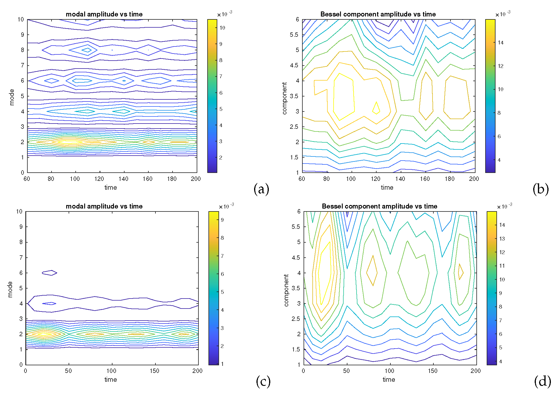
Figure 5.
(a) Total rate of deformation in the TQG model at ; (b) same for the decoupled 2D model (the image was zoomed in on the vortex).
Figure 5.
(a) Total rate of deformation in the TQG model at ; (b) same for the decoupled 2D model (the image was zoomed in on the vortex).
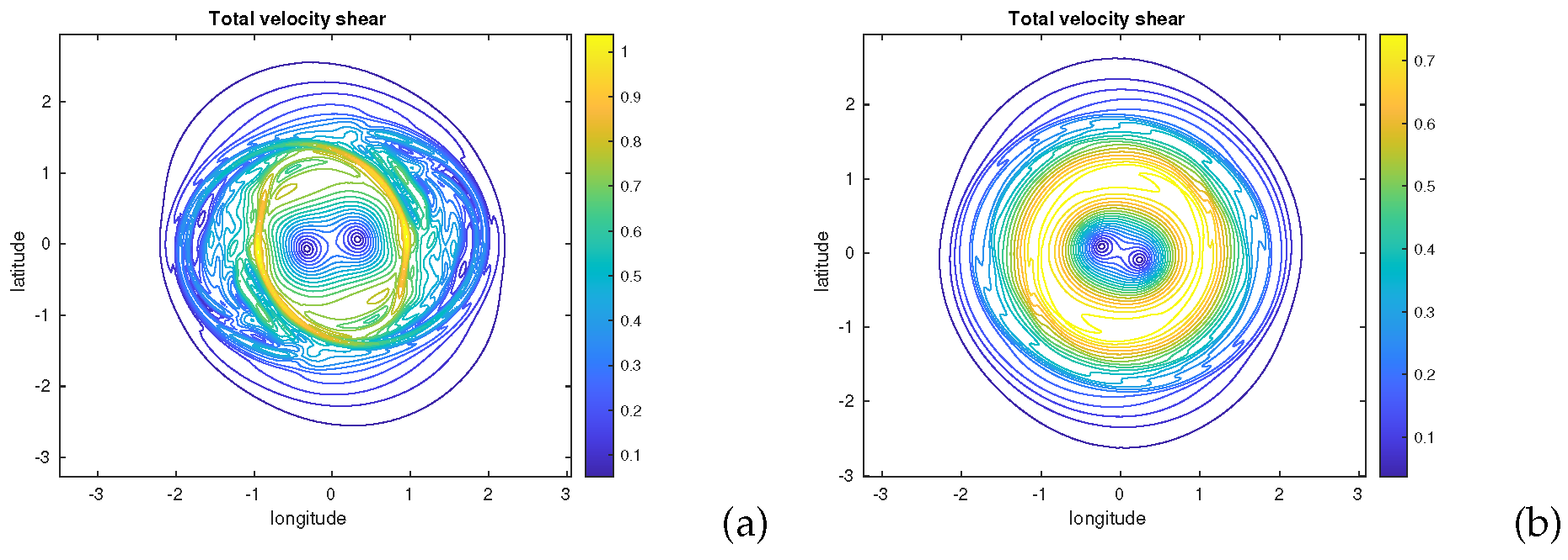
Figure 6.
Frontogenetic tendency in the TQG model at (zoom on the vortex).
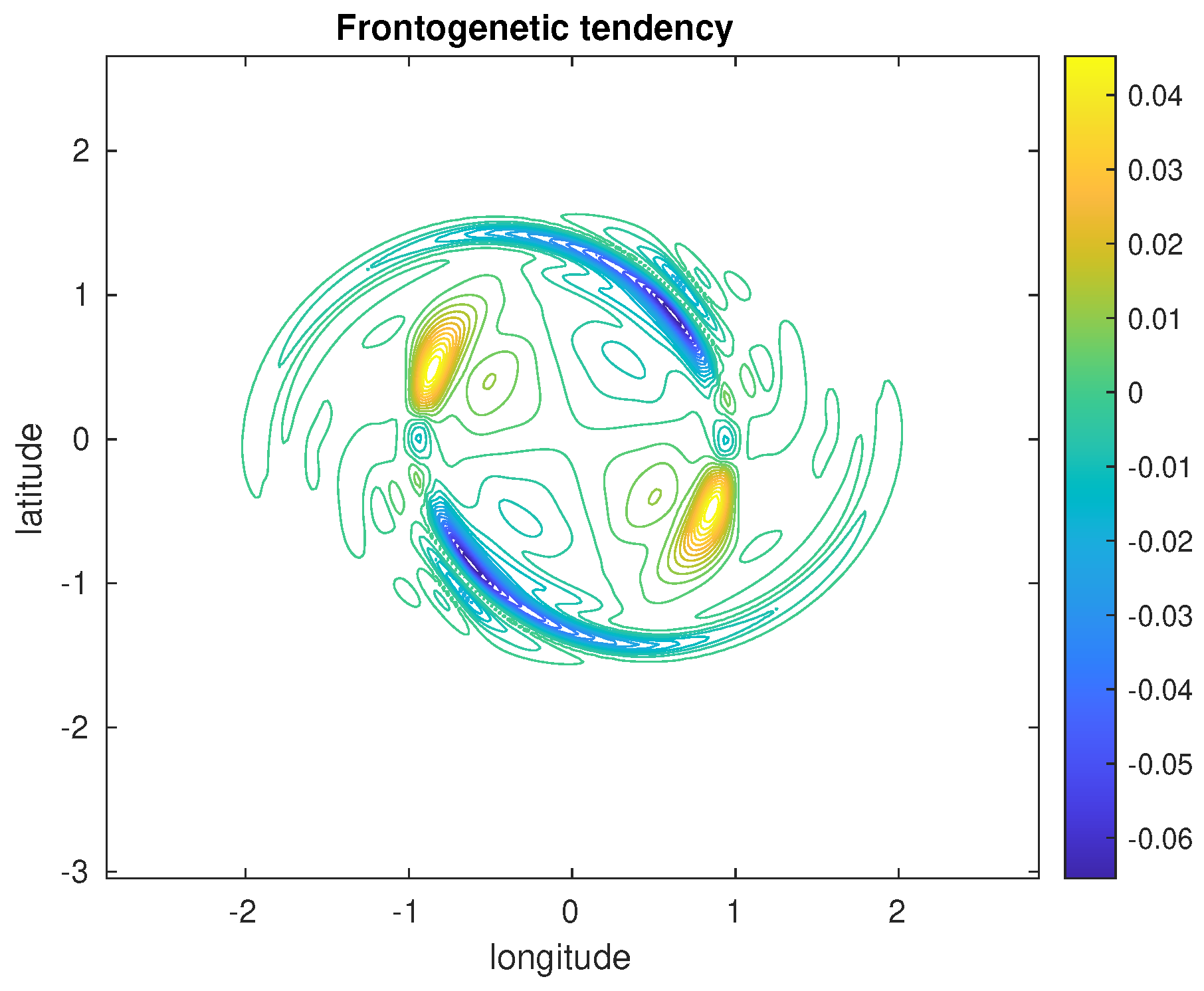
Figure 7.
(a) Nonlinear regimes in the plane for ; (b) vorticity and buoyancy maps for - in the turbulent tripole regime; (c) vorticity map for - in the dipolar breaking regime (2DP).
Figure 7.
(a) Nonlinear regimes in the plane for ; (b) vorticity and buoyancy maps for - in the turbulent tripole regime; (c) vorticity map for - in the dipolar breaking regime (2DP).
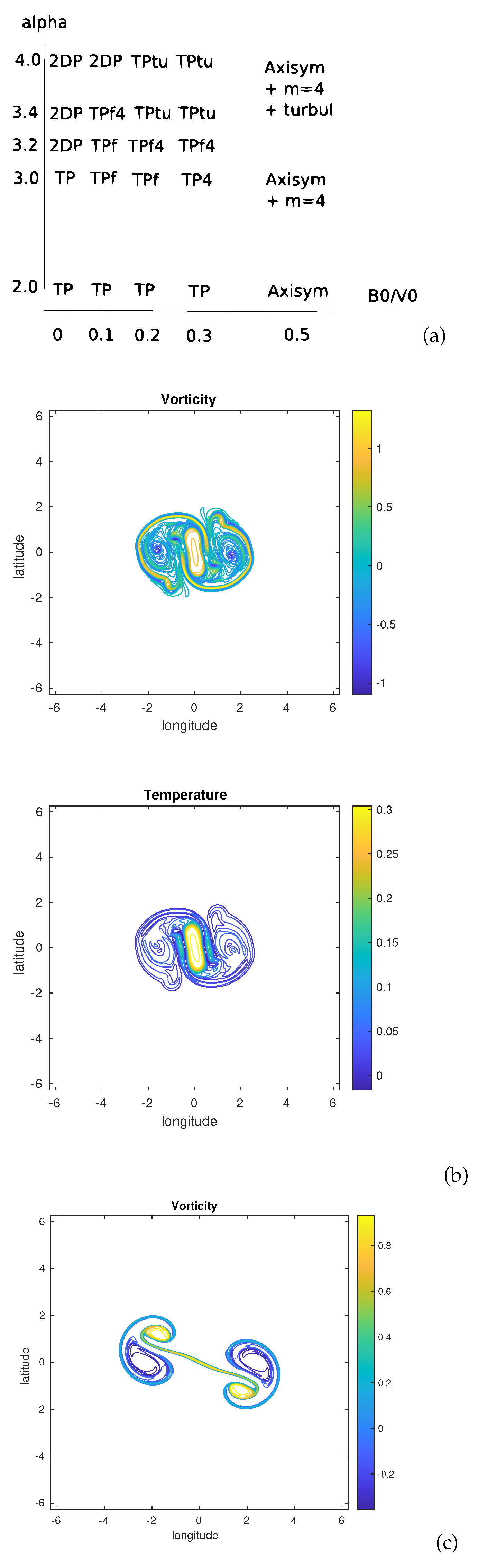
Figure 8.
End-states of simulations for a Gaussian vortex with and ; (a) Vorticity and buoyancy maps at for ; (b) vorticity and buoyancy maps at for ; (c) vorticity and buoyancy maps at for .
Figure 8.
End-states of simulations for a Gaussian vortex with and ; (a) Vorticity and buoyancy maps at for ; (b) vorticity and buoyancy maps at for ; (c) vorticity and buoyancy maps at for .
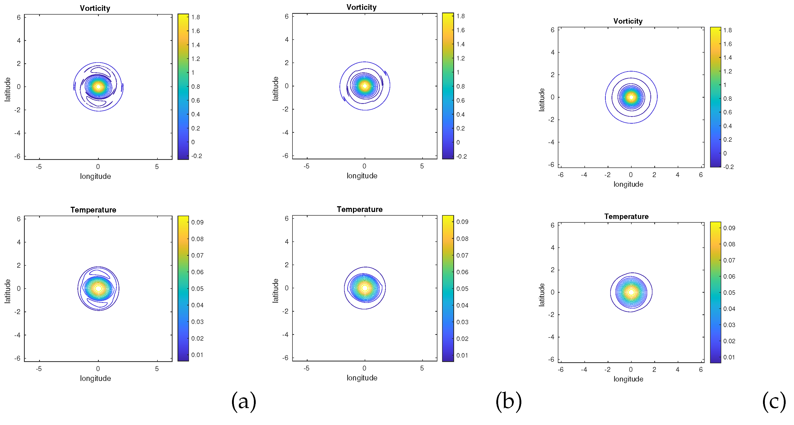
Figure 10.
(a) Table of end-states in the plane for power-exponential vortices perturbed with a mode (in the absence of stratification and of topography); (b) Vorticity and buoyancy maps at for a vortex with ; (c) vorticity and buoyancy maps at for a vortex with .
Figure 10.
(a) Table of end-states in the plane for power-exponential vortices perturbed with a mode (in the absence of stratification and of topography); (b) Vorticity and buoyancy maps at for a vortex with ; (c) vorticity and buoyancy maps at for a vortex with .
Disclaimer/Publisher’s Note: The statements, opinions and data contained in all publications are solely those of the individual author(s) and contributor(s) and not of MDPI and/or the editor(s). MDPI and/or the editor(s) disclaim responsibility for any injury to people or property resulting from any ideas, methods, instructions or products referred to in the content. |
© 2025 by the authors. Licensee MDPI, Basel, Switzerland. This article is an open access article distributed under the terms and conditions of the Creative Commons Attribution (CC BY) license (http://creativecommons.org/licenses/by/4.0/).
Copyright: This open access article is published under a Creative Commons CC BY 4.0 license, which permit the free download, distribution, and reuse, provided that the author and preprint are cited in any reuse.


