
Submitted:
16 January 2025
Posted:
17 January 2025
You are already at the latest version
Abstract
This work addresses the statistical mechanics of vortex gases and the thermodynamics of the initial formation (genesis) of tornado-like vortices. In particular, it discusses how the thermodynamics of discrete vortices in a quasi-two-dimensional (thin three-dimensional) boundary layer drives the creation of ``hairpins'' and ``cusp'' vortices, their two-dimensional rearrangement, and stretching of vorticity in the vertical direction that originates inside a turbulent boundary layer that leads to a tornado-like flow. Turbulence of that process is analyzed with the help of the vortex filament model and its connection to the fluid flow equations via the Hasimoto and Madelung transforms of the cubic nonlinear Schr\"{o}dinger and Gross--Pitaevskii equations. Finally, a formula for the local non-equilibrium entropy density flux associated with the development of quasi-two-dimensional turbulence in the boundary layer is provided.
Keywords:
quasi-two-dimensional turbulence
; thermodynamic fluxes
; entropy
; non-equilibrium thermodynamics
; nonlinear Schrödinger equation
; Gross Pitaevskii equation
; Madelung and Hasimoto transforms
; vortex stretching
MSC: 35Q30; 35Q31; 35Q55; 76D05; 76F40; 80A17; 94A17
1. Introduction
Investigation of atmospheric flows, especially the ones related to tornado-like events, requires a significant contribution from thermodynamic considerations, since a significant portion of a thunderstorm’s energy is generated by latent heat release associated with water vapor condensation. Citing [2]: “There is a strong nexus with thermodynamics, because these thunderstorms are driven by the phase change of water vapor. There are lots and lots of things other than pure fluid dynamics in this field.” To bypass the complications of storm thermodynamics, researchers and forecasters utilize various indices, in particular, combined mechanical and thermodynamic parameters, such as the fixed layer significant tornado parameter (STP). The STP is a composite index that includes the 0–6 km bulk wind difference (6BWD), the 0–1 km storm-relative helicity (SRH1), the surface based parcel convective available potential energy (sbCAPE), and the surface based parcel lifting condensation level (sbLCL). It is defined in the following way:
The sbLCL is set to 1.0 when sbLCL < 1000 m, and it is set to 0.0 when sbLCL > 2000 m; the 6BWD term is capped at a value of 1.5 for 6BWD > 30 m/s, and set to 0.0 when 6BWD < 12.5 m/s [3].
A majority of significant tornadoes (EF2 or stronger on the Enhanced Fujita scale [6]) have been associated with STP values greater than 1, while most non-tornadic supercells have been associated with values less than 1 in a large sample of Rapid Refresh (RAP) analysis proximity soundings. The RAP is a continental-scale NOAA hourly-updated assimilation/modeling system operational at the National Center for Environmental Prediction (NCEP) [4]. It covers North America and is comprised primarily of a numerical forecast model and an analysis/assimilation system to initialize that model. The definitions of the updated indices are given on the NOAA website [8]. A detailed discussion of the combined and other tornado indices is given in [9,10]. In particular, it is stated in [9]: “Forecasters and researchers are seeking a `magic bullet’ when they offer up yet another combined variable or index for consideration.”
One of the aims of this work is to establish a consistent thermodynamic approach aiming to bypass the ad-hoc nature of thermodynamic indices and develop a consistent model of non-equilibrium thermodynamic evolution in a tornado-like flow.
In addition to meteorological data obtained in recent decades, a large number of numerical simulations were recently carried out to identify storms that produce tornadoes (see [11,16] and the references therein). For example, in recent simulations with STP (generally considered ideal for tornado development), many cases produced only short-lived tornado-like vortices [16]. However, one particular simulation, referred to in [16] as “Storm 9,” led the author to suggest that a particular mechanism, the creation of “hairpins” and “cusps” in the boundary layer, related to a turbulence in the boundary layer, can lead to the generation of a tornado-like vortex. This turbulent boundary layer flow, which is driven by two-dimensional like vortices in a thin three-dimensional surface layer, then forms an inverse energy cascade to produce coherent (turbulent) structures that later are subject to vortex stretching and may produce a tornado (see [11]).
Further confirmation of the significance of thermodynamics then comes as well from concluding remarks in [16] on the presence of heat flux in a coherent structure environment to affect horizontal vorticity streaks and its importance in facilitating tornado-like vortices in real storms to accompany tornado forecasting when conditions favor hairpin vortices and (possibly cusps or any other coherent turbulent structures).
In this work, we attempt to develop a better understanding of how non-equilibrium thermodynamics accounts for low-level boundary turbulence that leads to generation of tornado-like vortices and their subsequent stretching.
We should note that in recent years studies of “standard” classical thermodynamics have developed in many branches influenced by non-equilibrium models in phenomenological and statistical formulations. In this paper, we will carefully specify the thermodynamical context in which we will use. For instance, in Section 3 and in Section 4 we address traditional thermodynamics via the local equilibrium hypothesis and the assumption of macroscopic fluctuations (see references therein). However, in Section 2 and Section 5 we use thermodynamics and statistical mechanics of vortex gases. We also emphasize that these two approaches are independent of one another even though there are some formal similarities.
The paper is organized as follows. In Section 2 we introduce and analyze the two-dimensional turbulence equivalence theory, where a highly singular vorticity field is well approximated by the interaction of point vortices and reflects important features of turbulence in the inverse energy cascade across the boundary layer. Based on that foundation, we then use a vortex filament approximation to find a governing equation driving the formation of “hairpins” mentioned earlier in this introduction. In Section 3 we outline the general thermodynamic theory in non-equilibrium settings, and we discuss thermodynamic potentials and why the entropy is the most fundamental thermodynamic variable in non-equilibrium thermodynamics (see also Section 4). Indeed, in Section 4 we outline the methods of macroscopic fluctuation that explain the additional terms in conservation laws and how they are related to the entropy change. Specifically, methods of macroscopic fluctuation are based on the fact that the probability of transition to a certain state depends on the change in entropy of the system. In Section 5 we use the analogy between the filament equation and its counterpart in the nonlinear Schrödinger equation developing it further to compare with (mathematical but not modeling) structure of the special case of the Gross–Pitaevskii equation. We apply the nonlinear Schrödinger equation to continue the investigation of singular vorticity fields with point vortices to describe three-dimensional vortex motion that is consistent with vortex stretching behavior. We also provide references there on the equivalence of the Schrödinger and Gross–Pitaevskii wave function and fluid flow equations via the Madelung and Hasimoto transforms. The benefits in this case come from the fact that vortex equations use more fundamental, potential-like quantities, such as the vortex density and the curvature, rather than the original fluid flow fields (velocity and vorticity), to describe flow singularities. The reason is that the velocity and vorticity fields suffer blow-ups that are difficult to model [19]. We also comment on a different approach used to obtain similar conclusions for tornado modeling developed in [18]. We conclude this section with calculation of a thermodynamic flux far from the equilibrium and provide a formula for the local entropy time rate that is applicable to study the non-equilibrium evolution on both the horizontal and vertical scales. Section 6 provides a detailed summary and discussion of implications of our model of tornado-like vortices.
2. Supercells, Self-Induction Filament Model, and Hairpins
We start by describing the mature stage of a supercell thunderstorm (see Figure 1), which features a rotating updraft known as a mesocyclone. At this mature stage, a wall cloud (not shown in the figure) descends from the base of the supercell beneath the mesocyclone. The mesocyclone’s updraft draws in warm, buoyant, and moist air through the wall cloud base. The rotation in the updraft creates a pressure deficit that helps to draw and lift surface air into the wall cloud.
As the moisture-laden air rises, it undergoes phase changes, releasing latent heat that intensifies the updraft. Eventually, this moisture freezes and is expelled from the sides or top of the mesocyclone. The forward flank and rear flank downdrafts are regions where this frozen precipitation falls; as it evaporates, it cools the surrounding air, making it negatively buoyant and contributing to the formation of downdrafts adjacent to the mesocyclone.
The storm’s movement allows the mesocyclone to ingest air that has not been evaporatively cooled. The boundaries between the incoming warm, moist air and the cooler, evaporatively cooled air are called the forward flank and rear flank boundaries or gust fronts. These gust fronts meet beneath the wall cloud as seen in the figure. The region between these boundaries, located below the wall cloud, is where tornadogenesis will occur.
Until recently it has been thought that vorticity produced baroclinically—possibly associated with vortex sheets formed in the downdrafts and tilted vertically—played the most important role in tornadogenesis. However, recent numerical simulations (see [16]) incorporating surface friction and resulting thermodynamic effects, including heat flux, suggest that other factors may play a critical role in a different mode of tornadogenesis. We will investigate evidence for this alternative mechanism, which involves features in the boundary layer such as the nearly two-dimensional turbulence, the formation of hairpin vortices, and the breakdown of the cyclostrophic balance.
Cyclostrophic balance refers to the equilibrium between the pressure gradient force and the centrifugal force. A critical step in tornadogenesis is the disruption of this balance due to surface friction. When surface friction reduces the centrifugal force, the pressure gradient force becomes dominant, causing an existing, wide, less intense vertical vortex to collapse into a narrow high-intensity filament.
Recently, it has been shown that tornado development might be enhanced by turbulence and the dynamics of vortical structures in the boundary layer [16]. Specifically, it is argued that boundary layer “coherent structures” such as “hairpins” and “cusps” [16,32,33,34] play a significant role in tornadogenesis. See Figure 2 for the steps in development of a “hairpin” vortex.
Cusps are the filaments between the two parallel counter-rotating segments of a hairpin (see the right image of Figure 2, Figure 3, and the right image of Figure 4).
For a shallow surface layer, their behavior can be approximated by a quasi-two-dimensional model (see Figure 3). The sequence of images showing the formation of cusps is shown in Figure 5.
The case of three-dimensional turbulence in a shallow layer that can be approximated as two-dimensional is called quasi-two-dimensional turbulence. We use this term later in Section 5 to describe the situation studied there. In two-dimensional flows, energy and enstrophy are conserved quantities. In these formulas, and are the velocity and vorticity fields, respectively, and denotes their space averages. The energy spectrum, , and the enstrophy spectrum, , are related via , which implies that in two dimensions the energy must cascade to larger scales and the enstrophy must cascade to smaller scales ([12,13,14,15,17]). The extent to which this fails to hold in three dimensions is related to whether turbulence in thin surface layers of the three space is quasi-two-dimensional or not (see [15,17]).
In this case, given the quasi-two-dimensional nature of the vortices (cusps), they do not dissipate (see [17]). Additionally, in two dimensions there is no vortex stretching. During the storm progression the cusps will be subject to stretching, which can lead to the storm intensification and possibly to a tornado-like vortex development. As the stretching occurs, the cusps unravel (see Figure 4), forming filaments which requires a transition from a quasi-two-dimensional turbulence model to a three-dimensional turbulence model. Due to the inverse energy cascade, the filaments concentrate into clusters of vorticity that satisfy the cyclostrophic balance conditions. The breakdown of cyclostrophic balance between the pressure gradient and the centrifugal forces leads to the collapse of these vorticity clusters into narrow high-energy filaments.
The simulations performed in [16] (see Figs. 7(c) and 8(c) in [16] or Figure 4 here) show what appear to be north-south oriented legs of hairpin vortices, with vertical spikes of east-west oriented vortices between the hairpin legs. The image of the corrugations (vertical vorticity spikes) suggests that the net vorticity in the quasi-two-dimensional turbulence would be zero provided the positive and negative vorticity legs have the same strength. A 12-hour burn-in that includes the Coriolis effect (due to the Earth’s rotation) is performed in [16], which leads to the positive vorticity leg having a larger vorticity value than the negative vorticity leg. Consequently, the net vertical vorticity is not zero. Following the burn-in, a thermal perturbation is added to initiate a storm. In the same study, another run without the Coriolis effect included is performed, which results in smaller mid- and upper-level winds in the pre-storm environment and leads to a weaker mesocyclone. The absence of tornadoes in this case is interpreted as being due to the effects on the mesocyclone strength rather than the equal strength of the anti-cyclonic and cyclonic legs of the vorticity spikes.
As the corrugations (vertical vorticity spikes) in the quasi-two-dimensional turbulence are tugged up into the mesocyclone (in a streamwise sense), the negative side of the vertical vorticity spike tilts 180 degrees aligns with the positive side and becomes positive, potentially amplifying the strength of the tornado.
The evolution of narrow, three-dimensional vortex filaments consistent with the Navier–Stokes equations is analyzed in [30]. In that work, the self-induction equation for , the position function of the center curve of a filament, is given by
where is the curve parameter, t is the (rescaled) time variable, is the curvature of the center curve, and is the binormal vector along the center curve of the filament (i.e., the cross product of the unit tangent and the unit normal vectors to the curve). Note that we use for the binormal vector instead of the standard to avoid confusion with the thermodynamic fluxes to be defined and used in the next section. The validity of the self-induction equation (1) rests on the following four assumptions, in which is the circulation around the filament, is the kinematic viscosity, is the vorticity, and is the radius of curvature of the center curve:
- the vorticity is nonzero only inside the filament of radius ;
- the radius satisfies ;
- the vorticity is large enough inside the tube so that as ;
- the radius of curvature is bounded strictly away from zero.
Note that in the self-induction case the length of the curve , representing the vortex filament, cannot increase in time and thus the dynamics described by (1) will not capture stretching effects.
Consider next the Hasimoto transform
where is the complex-valued filament function and is the torsion of the filament curve [30]. Recall that torsion can be viewed as a measure of the failure of a curve to be planar. A perturbation of (1) in the form
where is the center curve velocity field, together with the Hasimoto transform (2), then leads to the perturbed Schrödinger equation for the filament function :
The expression for the last term in (4) is given by formula (7.21) in [30] and since we will be mostly interested in the case , we won’t repeat it here. For the original self-induction case with , equation (4) turns into the nonlinear Schrödinger equation (with cubic nonlinearity)
Note from (2) that the magnitude of the filament function appearing in (4) and (5) is the curvature of the filament, i.e., . The cubic Schrödinger equation (5) has solutions (including explicit ones) that allow large values of and thus large curvatures. An example would be a hyperbolic secant solution (see, e.g., [31]). That indicates that the “hairpin” structures [16,32,33,34] appearing in the boundary layer and observed in [16] may appear as a result of boundary layer turbulence before stretching takes place.
Note that the initial formation of hairpins occurs in a relatively thin boundary layer. One estimate of its thickness ( meters) is provided in [16]. When the height of the boundary layer is relatively small (see more on that in Section 5), we may view this filament model as representing two-dimensional turbulence. We point out the similarity to the behavior of point vortices in two dimensions, where vorticity evolution can also be governed by other forms of the nonlinear Schrödinger equation. A recent work on verification of such analogies, particularly an analogy with the Gross–Pitaevskii equation, is presented in [35]. A deep mathematical analysis connecting fluid (Euler and Navier–Stokes) equations and various forms of the nonlinear Schrödinger equation is presented in [36].
To summarize, there is evidence for tornadogenesis mechanisms that involve phenomena occurring in the boundary layer. One such observed phenomenon is the formation, organization, and eventual stretching and intensification the vertical filaments between the legs of hairpin vortices. These filaments associated to hairpin vortices are not parts of vortex sheets and they are not a source of baroclinic vorticity. In addition, the results of the numerical simulations in [16] also serve as additional motivation for how to approach non-equilibrium aspects of tornado thermodynamics discussed in the next sections.
3. Entropy in Equilibrium and Non-Equilibrium Thermodynamics
In the standard thermodynamic theory the equation of state is , where S is the entropy and , , are extensive quantities that determine the state of a thermodynamics system in equilibrium. If a change happens infinitely slowly (quasi-statically), then the system moves to a different equilibrium state according to
where are the corresponding conjugate (intensive) quantities (forces) in the system under consideration (i.e., the partials of S with respect to the ’s). A simple thermodynamic system can be described by , where U is the internal energy of the system and V is the volume of the system. If the system is an ideal gas, then , where here and in what follows T is the absolute temperature and P is the pressure.
The first step to systems that are not in equilibrium is to employ the local equilibrium hypothesis, where all the (local thermodynamic) variables are well defined for a “small enough” system in a quasi-equilibrium state [20]. In the fluid dynamics context, such a “small enough” system is an air parcel with state variables dependent on the position and the time t, so that
In (6) we use lower-case letters for local thermodynamic variables that are functions of position and time. More precisely, s is the specific entropy (per unit mass), are the specific extensive variables (per unit mass), and stands for the change in the variables describing the air parcel. Note that in the non-equilibrium context we cannot assume a local constitutive equation and thus
where are the corresponding (local) conjugate variables, would not hold. To remedy this problem we recall that in non-equilibrium systems for each parameter we assign the (vector) thermodynamic flux , , that is not present in the standard equilibrium context. Following [20], we can replace (7) with an extended irreversible thermodynamics equation
where now do represent the conjugate local variables, and represent the conjugate local fluxes. When there is no significant transport of new chemical substances into the system, we can assume that all the fluxes are generated by the transport of the parameters associated with our system. However, non-equilibrium models with chemical transport will contain additional fluxes in the second sum on the right-hand-side of (8) (see [20]).
The non-equilibrium thermodynamic fluxes satisfy the transport equations
However, because of the non-equilibrium mesoscopic (see more below on that term) nature of the processes we consider, to account for strongly fluctuating terms we rewrite the thermodynamic fluxes in the form
where is a stationary flux of the parameter equipped with its own constitutive formula and where are the turbulent terms (a separate justification for that is given in Section 4). Thus, with the decomposition in (10), the transport equation (9) becomes
Note that the terms are responsible for the “mismatch” between macroscopic and microscopic descriptions, since they take place on different space and time scales. Such turbulent thermodynamic systems may be categorized as mesoscopic [20]. Note that similar mismatches due to fluctuations in the velocity field are called turbulent fluxes [21,22]. The turbulent thermodynamic fluxes do not satisfy any constitutive equations. Instead, they are replaced by Onsager reciprocal relations [23] (see also Chapter 7 in [20]) via
where are the Onsager coefficients matrices. Let us apply (8) (in the sense of (7.1) in [20]) to a local extended entropy function (case )
where is the local internal energy density and where is the local non-equilibrium heat flux associated with the vortex motion. Consequently,
where is the equilibrium reciprocal temperature and is the vector non-equilibrium equivalent of the reciprocal temperature.
For the general case of fluxes there needs to be an additional set of equations from experimental data. In the case of a heat flux, the Fourier law , where is the thermal conductivity, may not be applicable as non-equilibrium systems may have spatial and temporal non-local influence. Then the heat flux will depend on higher-order derivatives of temperature, or, conversely, the non-equilibrium temperature will depend on higher-order derivatives of the heat flux. In some cases, one can limit the memory effect to some “relaxation” time that leads to a Cattaneo’s type equation, e.g., . Note that the local extended non-equilibrium entropy is assumed to satisfy the following conditions: it is additive, it is a function of thermodynamic variables and fluxes, it is concave in the thermodynamic variables, and for each point of the system [20]. Under the Onsager linearity assumptions,
where v is the specific volume, , is the mass density, and is a function of the local internal energy u [20]. Then, combining (12) and (13), we obtain a formula for entropy production in the form
A detailed account of recent developments in understanding the irreversible entropy production is given in [24].
4. Mesoscopic Thermodynamics and Macroscopic Fluctuation
Tornado-like vortices, from radar observations and numerical simulation (see [11,16,25]) exhibit properties of a system far from equilibrium, so, on the mesoscopic level, when the system exhibits both macroscopic and microscopic features, we must understand how far from equilibrium that system is. The foundation of such analysis is to evaluate probabilities of various states far from the equilibrium. So, essentially, thermodynamics cannot ignore spatial and temporal “memory” as we indicated in Section 3. We recall that the statistical entropy of a system is defined by , where is the Boltzmann constant and W is the number of microstates corresponding to the macrostate with entropy . Then, solving for the number of microstates, we obtain . This serves as a basis for the Einstein formula that asserts that the probability of the state with entropy can be written as
where is a normalizing factor [26]. These ideas were developed by many researchers throughout recent decades and have been summarized in [27]. Eventually, the statistical entropy was replaced with a functional that depends on the fluctuations given by the thermodynamic fluxes (10). Then (15) becomes
where is heat delivered to the region as a result of the turbulent flux of the parameter (defined in (10)), and is the probability of the fluctuation of the system caused by that turbulent flux. According to [27],
where is the mobility matrix. In many cases, is quadratic in [27].
In [27,28] it is shown that if (16) holds, then the evolution of a system, subject to macroscopic fluctuations, must satisfy
where is the matrix “diffusion” internal field for the parameter , and the the “convection” external field due to the parameter . Then (11) and (17) imply
and the local turbulent thermodynamic flux is given by
In case of local equilibrium (see Section 3) the theory of microscopic stochastic dynamics [28] leads to an expression for the “diffusion” internal field in the following form:
where is the (local) Helmholtz free energy density per unit volume. Note that the values of CAPE, used in tornado prediction and analysis (see Section 1), are related to the Helmholtz free energy. We can use (18) to find the (local) equilibrium entropy density per unit mass induced by as
and compare (19) with non-equilibrium entropy in (14). However, (14) is in a form of differential and, since supplied heat is dependent on the path of the system, the calculation of the entropy itself (up to a constant) may present a challenge.
5. Vortex Stretching and an Asymptotic Filament Formula
In this section we analyze the vortex stretching driven by three-dimensional turbulence, and we also discuss the non-equilibrium thermodynamic properties associated with vortex stretching. Asymptotic form of the nonlinear Schrödinger filament equation is derived in [30] to allow for stretching. The original form of the self-induction ansatz (1) in that case has been replaced with a perturbed version
where is the expansion parameter, is the tangent vector to the centerline of the filament in the original (unperturbed) configuration ([37]), and is the perturbation term defined via
where is linear in the normal and binormal vectors in the unperturbed configuration (equation (1.8) in [37]), and where is a “non-local” term defined below in (21). It is non-local in the sense that it includes information from all the points on the centerline of the filament. It is important to mention that the asymptotic assumptions on scaling here are . These assumptions lead [30,37] to the asymptotic filament equation with self-stretching
where
where H is the Heaviside function. Note that in (20) the cubic term and the term compete on the same scale. Additionally, the Fourier transform of in (21) is , where and is the (irrational) Euler–Mascheroni constant, [30].
Below we use statistical mechanics of vortex gases. These ideas are motivated by the statistical mechanics of gases where the behavior of a large number of particles is simplified by making assumptions about the mean behavior of the collection, rather than trying to solve the system of equations for the interactions of each particle with all the others. The phase space of such a system contains information about the position and momentum of each particle, assumptions are made on the energy E and entropy S of the system, leading to a probability distribution on the phase space. In the case of fluid dynamics, the phase space is the set of all paths joining a pair of points, indicating vortices and the beginning and ending points. In the case of an ideal gas, the partition function is important in the probability distribution, where are the energies of the microstates indexed by i, and represents the inverse temperature. For fluid dynamics, vortex gases have a partition function of the form, , where the integral is taken over the phase space of all paths under consideration. H is the Hamiltonian of the system, this represents the energy of the system. In the case of vortex gases, negative temperatures imply the vortices are smooth, positive temperature vortices are balled up. For temperatures are plus or minus infinity and the vortices are Brownian paths. Note if is positive then . Straight vortices would have negative temperature in the vortex gas sense ([25,53,54]). Generally speaking, negative temperature vortices have high energy density and are "straight" or "smooth", while positive temperature vortices are balled up and dissipating. Negative temperature vortices are hotter than positive temperature vortices, with vortices that have the plus infinity = minus infinity temperatures in between. As a negative temperature () vortex cools down, it becomes less straight and begins to fold up, as it transfers energy to larger scales, eventually becoming fractal with temperature plus infinity = minus infinity temperature (), starting the Kolmogorov energy cascade to smaller scales (and/or possibly balling up, ) and dissipating ([25,29,52,53,54]). In order for the negative temperatures to occur, phase space must be bounded as well as the energy (see [29], pages 258–260). In section 7.5 of [30] it is shown that two nearly parallel vortex filaments of opposite circulation are unstable. In the case of point vortices in a bounded region, if two point vortices have opposite circulations and negative temperature, then they will move away from each other toward the boundary.
In the discussion below, we consider two types of vortices: hairpin vortices and vertical straight filament vortices. The assumptions on filaments made in Section 2 and earlier in this section are made for hairpins. The formation of hairpin vortices from the interaction of a helical filament alined perpendicular to a background strain flow is mentioned below. Parallel vertical vortices are analogous to a corresponding set of point vortices in the plane (see section 7.3 of [30]) in that they satisfy the same equations. From the images in this paper we see these two types of vortices, hairpin vortices and vertical straight filament vortices, occur together. The filament vortices form a cusp located between the legs of the hairpin vortex legs (see the right image of Figure 4). The cusps are vortices formed from line tightly folded vortices. In the region of the cusps they are straight. We assume this close interaction brings the two types of vortices into a vortex gas quasi-equilibrium so they have the same temperature in the vortex gas sense. We assume the temperature is negative. We assume the flow evolves in a shallow layer above a bounded region on the surface plane beneath a supercell.
The perturbation of the cubic nonlinear Schrodinger equation that models the time evolution up to the birth of the “hairpin” and “cusps” vortices, is given by . This equation models “the birth” of “hairpins” and strong kinks (“cusps”) in the vortex filament from the interaction of the nonlocal operator (representing a strain flow) and the cubic nonlinearity ([38]) and “the conditions of the asymptotic theory become invalid as the hairpin vortex is born” ([38]). This is because the curvature exceeds the assumed bounds in Section 2. In [38] the authors discuss in detail the evolution up to that time. This necessitates the use of a different nonlinear Schrödinger Equation to model the “cusps”.
We now make assumptions (section 7.4 of [30]) on the structure of vortex filaments that prevents infinite energies from occurring. Assume , where is a parameter along the z-axis,
(1) The wavelength of perturbations is much longer than the separation distance.
(2) The separation distance is much larger than the core thickness.
The centerline of each nearly parallel vortex filament has the asymptotic form,
.
Each vortex filament has a cross sectional core radius satisfying,
, , .
From these conditions one has, the separation distance between vortices is , and the wavelength of perturbations is .
For the time being assume the vortices are all nearly parallel to the vertical direction. The equation governing a single such vortex is: (section 7.4 of [30]). This does not have a cubic nonlinearity but a minus one nonlinearity. Pairs of counter rotating vortices that satisfy this equation are shown to be unstable in section 7.5 of [30]. If the vortices are vertical and parallel to the z-axis, this equation reduces to (see section 7.3 of [30]). This is the same equation satisfied in two dimensions by point vortices. As long as the vortices are straight and parallel to the z-axis, they will behave like point vortices. Hence, the term quasi-two dimensional turbulence is used to describe 3 dimensional turbulence in a shallow surface layer, when the vortices can be approximated as vertical and straight. Approximate the cusp vortices in the furrows between the legs of the hairpins by straight filament vortices (see the right image of Figure 4). The furrows act like a local boundary for the cusps, this keeps them from unfolding and spreading out. We assume the temperature will be negative. In this situation there is an inverse cascade of energy to larger scales, and larger coherent structures tend to form, such as “hairpins” and “cusp” vortices. Assume in addition that the vertical vortices are in vortex gas equilibrium with the hairpin legs. It is shown in [30] that the family of nearly parallel vortices form a Hamiltonian system with conserved quantities. If we consider a single such vortex and assume it has a stretching background flow of the same form as in the cubic Nonlinear Schrödinger Equation, this vortex is in cyclostrophic balance (balance between the pressure gradient force and the centrifugal force). In the analysis below we grossly simplify the situation by ignoring the effects of the term to see some of the effects of the two-dimensional assumption. In the analysis below the range the of negative temperatures may be affected by this assumption.
In applying the quasi-two dimensional turbulence ideas we use a two dimensional model. If we consider the special case of a vortex parallel to the vertical direction, then following the above discussion, we approximate the vortex, using the two dimensional theory, as analogous to a point vortex. The two-dimensional theory is developed in [42,43]. This theory incudes a range of negative temperatures. The two dimensional theory motivated a three-dimensional theory of [39], which does not include negative temperature, however, a subsequent paper [44] allows a small range of negative temperatures provided the vortex has a fractal cross-section. In [42] they consider a N-vortex system in a bounded domain in with the associated canonical Gibbs measure, at inverse temperature . They prove that, in the limit , , , where (here denotes the vorticity intensity of each vortex), the one-particle distribution function , , converges to a superposition of solutions of the following Mean Field Equation (MFE): ; , , where is the stream function. Further in the paper they develop the following version of the two dimensional theory.
Consider a system of N vortices, with intensity , and . The equation of motion is , , where . The Hamiltonian (Energy) is , the associated Gibbs measure is , where is the partition function.
For a disc domain , the solutions of the MFE can be found and the concentration as . It can also be shown the concentration exists in a simply connected domain sufficiently close to a disk. There are regions for which the concentration does not occur ([43], page 238). Convergence to a smooth solution is also possible ([42]).
If we consider the special case of a vortex parallel to the vertical direction, then the associated partition function is , where is a narrow region with a smooth boundary representing the region (the furrow) between the adjacent hairpin legs. Given that there are many hairpins, there would be many such domains. Assuming the vertical vortices have negative temperature. The image (see the right image of Figure 4) of the corrugations (vertical vorticity spikes) suggests that the vorticity in the quasi-two-dimensional turbulence is zero, provided the positive and negative vorticity legs have the same strength. Markowski, in [16], does a 12-hour burn-in that includes Coriolis effects (planetary vorticity), this leads to the positive vorticity leg having a larger vorticity value than the negative vorticity leg. Consequently, the vertical vorticity induced by the spike is not zero. We think of the vertical vorticity spikes as straight vertical filaments. We think of the turbulent boundary layer as made up of these filaments. We use the two-dimensional turbulence model of [42,43] discussed above to model this situation. We assume the vorticity spikes in the corrugations, cluster into larger filaments with cyclonic and anti-cyclonic legs (the right image of Figure 4). As the larger clusters in the corrugations (vertical vorticity spikes) in the quasi-two-dimensional turbulence are tugged up into the mesocyclone (in a streamwise sense), the negative side of the vertical vorticity spike tilts 180 degrees aligns with the positive side and the vorticity becomes positive (the left image of Figure 4). As this happens and the vortex stretches we move from a quasi-two-dimensional model to a three-dimensional model. We assume the resulting vortex is in cyclostrophic balance (balance between the pressure gradient force and the centrifugal force). The surface friction along with the stretching and rotation of the collection causes the centrifugal force to weaken, killing off the balance between the pressure gradient force and the centrifugal force and then to form a vortex that collapses, as the pressure gradient force dominates, to a narrow filament with high energy density. If we think of the entropy as measuring randomness in the vortex, then when the vortex collapses the randomness decreases, , and the energy density increases, . Therefore, these vortices have a negative temperature state, . These vortices are called super critical or suction vortices. These vortices could be approximated by a delta function supported(concentrated) on a vertical segment. These vortices may lead to a tornado via three dimensional turbulence: the stretching of a negative temperature vortex leading to the transfer of energy to larger scales via folding, and as the folding continues leading to the eventual dissipation of energy via the Kolmogorov cascade, a direct energy cascade to smaller and smaller scales without lower bound (see ([25,53,54])). The processes described in the above paragraphs may be occurring repeatedly in the region below the supercell and mesocyclone.
This might be described by the following narrative. The mesocyclone cyclonic circulation weakly couples with the surface flow via viscous interactions between the intermediary layers. This produces a region outside the region underneath the mesocyclone base, of gradual cyclonic flow up to the mesocyclone base. For flow near the surface, that is nearly horizontal into this region, gives a background strain flow. Using the Majda and Klein model (see chapter 7 of [30] and [37,38]), this strain flow gives rise to hairpins. As the hairpins and cusps accumulate and flow closer to the mesocyclone base, they begin to circulate cyclonicly. Continuing to move closer to the region under the mesocyclone, the vertical cusps begin to unravel going through vortex breakdown and to spiral inward toward a common center. This leads to clusters of vertical vortices near the surface under the mesocyclone possibly leading to tornado genesis, the tornadoes intensification or maintenance.
In the video “Mays’s Fury” (see [5]) which documents the coverage of a violent tornado outbreak on May 3rd, 1999, the video shows (41st minute) a nearly horizontal vortex in or near a tornado while the tornado crosses interstate I-35. In addition, the horizontal vortex is visible in the region where the tornado appears to be the most intense. This is suggestive of a hairpin leg vortex in or adjacent to the tornado and the associated unravelled narrow vertical filament vortices, moving into the tornado, causing the tornado to intensify or maintain its intensity.
Since last two terms on the right-hand of (20) have the same scaling, we wish to investigate further the properties of the cubic nonlinear Schrödinger equation similar to (20). To gain the additional insight, the following discussion replaces the cubic nonlinear Schrödinger equation (20) used by [37,38] with the Gross–Pitaevskii equation (22). Note that the term defined in (21) is now replaced by a simpler linear term . In addition, we note that while we pursue a quantum mechanical analogy, we do not claim any quantum mechanical effects. The resulting equations describe the model at most up to the “birth” of “hairpins” and “cusps”. In [36] it is shown that the Madelung and Hasimoto transforms establish equivalence of the Gross-Pitaevskii and nonlinear Schrödinger equation classes to Newton’s and fluid flow equations including the Euler and Navier–Stokes equations. In [45] many features of turbulent vortices were obtained using numerical simulations of the solutions of the Gross–Pitaevskii equation. We will write that equation in a dimensionless form as [36,46]
where the unknown is the wave function, is an external (given) potential and . The wave function can be rewritten in terms of its magnitude and phase as
The Madelung transform establishes a connection between the solutions of (22) and the equations of fluid flow via
where is the vortex density. In [36] it is shown that the Hasimoto transform (2) is the Madelung transform in one dimension (Proposition 17 in [36]). In [47] it is demonstrated that the solutions of the Gross–Pitaevskii equation, after application of the Madelung transform, satisfy the Euler equations, and [48] shows that the inverse Madelung transform turns Euler equations into the Gross–Pitaevskii equation. One of the arguments in [45] in favor of the Gross–Pitaevskii equation to describe turbulence is the similarity of the flow profiles. For example, axisymmetric solutions of (22) admit a Rankine combined vortex, e.g., in the Equation (11) and Figure 6, 7 in Section 3.2 of [45]. These processes are also associated (in quantum and classical case) with irreversible entropy production (as shown in [24]).
The equivalence between the Euler equations (zero viscosity) and the Gross–Pitaevskii equation indicates that (similarly to densely packed sources of rotation perpetrated by Bose–Einstein statistical distribution) the turbulent interaction includes a “discrete-like” component associated with zero entropy and zero viscosity [45].
It has been established that, even when a system is very far from equilibrium, it is “aware” of what the equilibrium states are [49]. The dimensionless Gross–Pitaevskii equation (22) allows one to find the stationary states via separation of spatial and temporal variables by seeking solutions of the form
Substituting (23) into (22), we obtain an eigenfunction problem for
where is the corresponding eigenvalue. Thus we expect the eigenstates to be the observable states during non-equilibrium vortex evolution.
While the hierarchy of the cubic nonlinear Schrödinger equations (including the Gross–Pitaevskii equation) has been widely researched [50] and the connection between the fluid flow equations and the cubic nonlinear Schrödinger equation has been investigated (as discussed in Section 2 and the references therein), there is only statistical evidence about a connection between the two-dimensional turbulent flow and the Gross–Pitaevskii equation (22) as investigated in [35]. However, if we accept that analogy and assume that, under certain conditions,
then we can calculate the local non-equilibrium entropy density (see [51,52]) via
where is normalized and solves (20) and (22) (if (24) holds).
Work [18] developed a theory of the entropic balance, based on variational principles under assumptions of short time scales for phase changes. It provides a variational derivation of the governing equations in the thermodynamic context and includes a discussion of how entropic balance can be affected by a highly non-equilibrium storm environment. In particular, it states that entropy balance must be complemented with a term accounting for non-equilibrium entropy fluctuations, i.e.,
where is the term similar to the term in the equation (5.6b) in [18]. Therefore, if we use (25) to compute the non-equilibrium entropy rate
we then find, by substituting (27) into (26), the local non-equilibrium entropy flux, due to the turbulent fluctuation, as
If the entropy flux is concentrated in the boundary layer, where the pressure changes (on average) are insignificant, we can use (28) to estimate the heat supply to a region of the two-dimensional turbulent flow as
where is the heat capacity at constant pressure.
6. Summary
To have a realistic model of the evolution of a three-dimensional vortex we used a quasi-two-dimensional approach which is reasonable in the case when the foundational vertical filaments , i.e. furrows of "cusps" [16,32,33,34] move in a thin three-dimensional region which can be approximated by a two-dimensional model (see the right image of Figure 4). As indicated in the previous section, the turbulence is quasi-two-dimensional and hence exhibits an inverse energy cascade forming coherent structures such as "hairpins" and "cusps" (see the right image of Figure 4). As the cusps are captured by the updraft, energy accumulates at larger scales, while we assume the flow is in cyclostrophic balance. If the surface friction kills off the cyclostrophic balance between the pressure gradient force and the centrifugal force, allowing the pressure gradient force to dominate, the vortex collapses to a narrow filament. The filament, stretched by the updraft, could then transfer energy to a deeper region of the flow, possibly leading to tornadogenesis [25,53,54]. If most of the turbulence is focused in the boundary layer [16], one can expect that, instead of gradual tilting of vorticity in vertical direction (which would happen if turbulent energy was low in the boundary level), almost all turbulence will develop in the boundary layer (7.5 m according to [16]). Thus the formed low-level coherent structures (cusps) would then undergo unraveling and stretching in the vertical direction (see the right image of Figure 4).
The non-local term in the asymptotics (20) of the nonlinear Schrödinger filament equation generates the two-dimensional turbulence that develops in the boundary layer and results in the subsequent stretching of the vorticity that does not require a separate model, and the process can be described by the evolution of the vortex density. Hairpin vortices form in a transitional boundary layer, possibly due to the separation of the flow over the boundary layer. The hairpin vortices consist of two counter-rotating streamwise vortices connected at the region rising further up which resembles a slightly curved "hairpin". In the simulations of Markowski [16] the vorticity that is ingested into the tornado comes from cusps forming between the two counter rotating vortices, possibly associated to hairpin vortices. An example of how the asymptotics can produce separation in the boundary layer and thus create vorticity is given in [55] (section 2.2, page 67); see also [32,33,34]. The conversion from quasi-two-dimensional turbulence to three-dimensional turbulence may be driven by stretching mechanisms as described in [16,25,53,54]. This stretching unravels the tightly folded vortices that form the cusps (see the first image of Figure 4).
It has been suggested that the surface heat flux and surface horizontal windspeed might be useful as quantities in forecasting tornadogenesis [16]. In this paper we have discussed thermodynamic fluxes (including composite indices) in the context of non-equilibrium thermodynamics as related to the onset of quasi-two-dimensional turbulence in the boundary layer and subsequent vortex stretching. As indicated above, one of the possible mechanisms for tornadogenesis is forming of "hairpins" and "cusps". These coherent structures may initiate in the boundary layer, under the influence of the surface heat flux and continuing turbulence and then in particular, the "cusps" may have their vorticity unravel, while stretching in the vertical direction takes place on a different time scale. So, the information on the thermodynamic (including composite) indices discussed in Section 1 is available only after turbulence in the boundary layer has developed. We know that the observable non- equilibrium states are not chaotic, but rather must be stationary [49] and possess an analog of a Lyapunov function [56], in particular, for non-equilibrium thermodynamic quantities such as entropy. So, even if the system is far from equilibrium, we can use turbulent fluxes to describe tornado-like vortices. Therefore, at the boundary level the turbulent fluxes described in (10) are well defined and we can use (27)–(29) to find the local non-equilibrium entropy rate, associated local non-equilibrium entropy flux, and heat supply, respectively.
The entropy is closely related to potential temperature (see [21] and also the various definitions of potential temperature and the definition (3.23) of entropy temperature in [57]). If the surface temperature is high, then the gradient of potential temperature should point opposite the direction of the heat flux. Also, simulations [16] show tornado formation after globs of "cusps" crossed to the cool side of the forward flank boundary, where the vertical gradient of the potential temperature (closely related to entropy) would have the largest magnitude. Hence, the heat would flow upward, dragging the "cusps" up as well, possibly leading to tornadogenesis.
References
- Zambri, H.; Eslam, R.L. Generation, Evolution, and Characterization of Turbulence Coherent Structures. Turbulence and Related Phenomena. Chapter 4. Turbulence and Related Phenomena 2018. [CrossRef]
- Cutlip, K. Interview with Richard Rotunno, a Senior Scientist at UCAR. Weatherwise 2015, May/June, 56–57.
- NOAA. Significant Tornado Parameter (fixed layer). https://www.spc.noaa.gov/exper/mesoanalysis/help/help_stor.html. Accessed: 2024-06-30.
- NOAA. Rapid Refresh Products. http://www.nco.ncep.noaa.gov/pmb/products/rap. Accessed: 2024-06-30.
- May’s Fury - May 3, 1999 Oklahoma Tornado Outbreak (KFOR-TV Documentary) https://www.youtube.com/watch?v=E5Dw3tXcIvA. Accessed: 2024-12-10.
- https://www.weather.gov/oun/efscale. Accessed: 2024-11-02.
- https://en.wikipedia.org/wiki/Rear_flank_downdraft. Accessed: 2024-11-02.
- NOAA. Composite Indices. https://www.spc.noaa.gov/exper/mesoanalysis/. Accessed: 2024-06-30.
- III, C.A.D.; Schultz, D.M. On the use of indices and parameters in forecasting severe storms. Electronic J. Severe Storms Meteor. 2006, 1, 1–14. [Google Scholar]
- Grams, J.S.; Thompson, R.L. Regional to Mesoscale Influences of Climate Indices on Tornado Variability. Weather and Forecasting 2012, 27, 106–123. [Google Scholar] [CrossRef]
- Orf, L.; Wilhelmson, R.; Lee, B.; Finley, C.; Houston, A. Evolution of a long-track violent tornado within a simulated supercell. B. Am. Meteorol. Soc. 2017, 98, 45–68. [Google Scholar] [CrossRef]
- Batchelor, G.K. Computation of the energy spectrum in homogeneous two-dimensional turbulence. Phys. Fluids 1969, 12(12), II–233. [Google Scholar] [CrossRef]
- Kraichnan, R.H. Inertial ranges in two-dimensional turbulence. Phys. Fluids 1967, 10(7), 1417–1423. [Google Scholar] [CrossRef]
- Kraichnan, R.H. Inertial-range transfer in two-and three-dimensional turbulence. J. Fluid Mech. 1971, 47(3), 525–535. [Google Scholar] [CrossRef]
- Kraichnan, R.H. Statistical dynamics of two-dimensional flow. J. Fluid Mech. 1975, 67(1), 155–175. [Google Scholar] [CrossRef]
- Markowski, P.M. A New Pathway for Tornadogenesis Exposed by Numerical Simulations of Supercells in Turbulent Environments. J. Atmos. Sci. 2024, 81, 481–518. [Google Scholar] [CrossRef]
- Alexakis, Alexandros Quasi-two-dimensional turbulence. Reviews of Modern Plasma Physics 2023, 71, 31–46. [CrossRef]
- Sasaki, Y. Entropic Balance Theory and Variational Field Lagrangian Formalism: Tornadogenesis. J. Atmos. Sci. 2014, 71, 2104–2113. [Google Scholar] [CrossRef]
- Elgindi, T.M. Finite-time singularity formation for C1,α solutions to the incompressible Euler equations on R3. Annals of Mathematics (2) 2021, 194, 647–727. [Google Scholar] [CrossRef]
- Lebon, G.; Jou, D.; Casas-Vazquez, J. Understanding Non-Equilibrium Thermodynamics; Springer-Verlag, New York, 2008.
- Holton, J.R.; Hakim, G.J. An Introduction to Dynamic Meteorology, sixth ed.; Academic Pres, 2019.
- Dokken, D.P.; Shvartsman, M.M., Time averaging, hierarchy of the governing equations, and the balance of turbulent kinetic energy.In Mathematical and Physical Theory of Turbulence; Cannon, J.; Shivamoggi, B.K., Eds.; Taylor & Francis Group, LLC, 2006; pp. 155–164.
- Giordano, S. Entropy production and Onsager reciprocal relations describing the relaxation to equilibrium in stochastic thermodynamics. Physical Review E 2021, 103, 05216–05229. [Google Scholar] [CrossRef] [PubMed]
- Landi, G.T.; Paternostro, M. Irreversible entropy production: From classical to quantum. Rev. Mod. Phys. 2021, 93, 035008–035066. [Google Scholar] [CrossRef]
- Bělík, P.; Dokken, D.; Shvartsman, M.M.; Bibelnieks, E.; Laskowski, R.; Lukanen, A. Equilibrium Energy and Entropy of Vortex Filaments in the Context of Tornadogenesis and Tornadic Flows. Open J. Fluid Dyn. 2023, 13, 1446–176. [Google Scholar] [CrossRef]
- Einstein, A. Theorie der Opaleszenz von homogenen Flüssigkeiten und Flüssigkeitsgemischen in der Nähe des kritischen Zustandes. Annalen der Physik 1910, 33, 1275–1298. [Google Scholar] [CrossRef]
- Bertini, L.; Sole, A.; Gabrielli, D.; Jona-Lasinio, G.; Landim, C. Macroscopic Fluctuation Theory. Rev. Mod. Phys. 2015, 87, 593–636. [Google Scholar] [CrossRef]
- Eyink, G.; Lebowitz, J.L.; Spohn, H. Hydrodynamics of stationary non-equilibrium states for some stochastic lattice gas models. Comm. Math. Phys. 1990, 132, 253–283. [Google Scholar] [CrossRef]
- Paul K. Newton N-Vortex Problem: Analytical Techniques; Springer, 2001.
- Majda, A.J.; Bertozzi, A.L. Vorticity and Incompressible Flow; Cambridge University Press, 2002.
- Farag, N.G.A.; Eltanboly, A.H.; El-Azab, M.S.; Obayya, S.S.A. On the Analytical and Numerical Solutions of the One-Dimensional Nonlinear Schrödinger Equation. Mathematical Problems in Engineering 2021, 2021, 3094011, [https://onlinelibrary.wiley.com/doi/pdf/10.1155/2021/3094011]. [Google Scholar] [CrossRef]
- Adrian, R.J. Hairpin vortex organization in wall turbulence. Phys. Fluids 2007, 19, 041301. [Google Scholar] [CrossRef]
- Bernard, P.S. The hairpin vortex illusion. Journal of Physics: Conference Series 2011, 318, 062004. [Google Scholar] [CrossRef]
- Bernard, P.S. On the inherent bias of swirling strength in defining vortical structure. Phys. Fluids 2019, 31, 035107. [Google Scholar] [CrossRef]
- Müller, N.P.; Krstulovic, G. Exploring the Equivalence between two-dimensional Classical and Quantum Turbulence through Velocity Circulation Statistics. Phys. Rev. Lett. 2024, 132, 094002. [Google Scholar] [CrossRef] [PubMed]
- Khesin, B.; Misiolek, G.; Modin, K. Geometric hydrodynamics via Madelung transform. PNAS 2018, 115, 2104–2113. [Google Scholar] [CrossRef] [PubMed]
- Klein, R.; Majda, A.J. Self-stretching of a perturbed vortex filament I. The asymptotic equation for deviations from a straight line. Physica D 1991, 49, 323–352. [Google Scholar] [CrossRef]
- Klein, R.; Majda, A.J. Self-stretching of a perturbed vortex filament II. The structure of solutions. Physica D 1991, 53, 267–294. [Google Scholar] [CrossRef]
- Lions, P.L.; Majda, A.J. Equilibrium Statistical Theory for Nearly Parallel Vortex Filaments. CPAM 2000, 53, 76–142. [Google Scholar] [CrossRef]
- Klein, R.; Majda, A.J.; Damodaran, K. Simplified equations for the interaction of nearly parallel vortex filaments. J. Fluid Mech. 1995, 288, 201–248. [Google Scholar] [CrossRef]
- Klein, R.; Majda, A.J.; McLaughlin, R.M. Asymptotic equations for the stretching of vortex filaments in a background flow field. Phys. Fluids A 1992, 4, 2271–2281. [Google Scholar] [CrossRef]
- Caglioti, E.; Lions, P.L.; Marchioro, C. ; Pulvirenti, M A Special Class of Stationary Flows for Two-Dimensional Euler Equations: A Statistical Mechanics Description. Commun. Math. Phys. 1991, 143, 501–525. [Google Scholar] [CrossRef]
- Caglioti, E.; Lions, P.L.;Marchioro, C.; Pulvirenti, M A Special Class of Stationary Flows for Two-DimensionalEuler Equations: A Statistical Mechanics Description. Part II. Commun. Math. Phys. 1995, 174, 229–260.
- Flandoli, F.; Gubinelli, M. The Gibbs ensemble of a vortex filament. Probab. Theory Relat. Fields 2002, 122, 317–340. [Google Scholar] [CrossRef]
- Barenghi, C.F., Tangled Vortex Lines: Dynamics, Geometry and Topology of Quantum Turbulence. In Knotted Fields; Ricca, R.L.; Liu, X., Eds.; Springer Nature Switzerland, 2024; pp. 243–279.
- Bao, W.; Cai, Y. Mathematical theory and numerical methods for Bose–Einstein condensation. Kinetic and Related Models 2013, 6, 1–135. [Google Scholar] [CrossRef]
- Roitberg, A.; Ricca, R.L. Hydrodynamic derivation of the Gross–Pitaevskii equation in general Riemannian metric. J. Phys. A: Math. Theor 2021, 54, 315201. [Google Scholar] [CrossRef]
- Carr, L.D.; Miller, R.R.; Bolton, D.R.; Strong, S.A. Nonlinear scattering of a Bose–Einstein condensate on a rectangular barrier. Physical Review A 2012, 86, 023621. [Google Scholar] [CrossRef]
- Jarzynski, C. Nonequilibrium Equality for Free Energy Differences. Phys. Rev. Lett. 1997, 78, 2690–2693. [Google Scholar] [CrossRef]
- Chen, T.; Pavlović, N. Derivation of the cubic NLS and Gross–Pitaevskii hierarchy from manybody dynamics in d=3 based on spacetime norms. Ann. Henri Poincaré 2014, 15, 543–588. [Google Scholar] [CrossRef]
- Madeira, L.; García-Orozco, A.D.; dos Santos, F.E.A.; Bagnato, V.S. Entropy of a Turbulent Bose–Einstein Condensate. Entropy 2020, 22, 22090956. [Google Scholar] [CrossRef]
- Chorin, A.J. Vorticity and Turbulence; Springer-Verlag, New York, 1994.
- Bělík, P.; Dokken, D.; Potvin, C.; Scholz, K.; Shvartsman, M. Applications of Vortex Gas Models to Tornadogenesis and Maintenance. Open J. Fluid Dyn. 2017, 7, 596–622. [Google Scholar] [CrossRef]
- Bělík, P.; Dahl, B.; Dokken, D.; Potvin, C.; Scholz, K.; Shvartsman, M. Possible implications of self-similarity for tornadogenesis and maintenance. AIMS Math. 2018, 3, 365–390. [Google Scholar] [CrossRef]
- Chorin, A.J.; Marsden, J.E. A Mathematical Introduction to Fluid Mechanics; Springer-Verlag, New York, 1992.
- Bulíček, M.; Málek, J.; Průša, V. Thermodynamics and Stability of Non-Equilibrium Steady States in Open Systems. Entropy 2019, 21, 21070704. [Google Scholar] [CrossRef] [PubMed]
- Hauf, T.; Höller, H. The Dependence of Core Radius on Swirl Ratio in a Tornado Simulator. J. Atmos. Sci. 1987, 44, 2887–2901. [Google Scholar] [CrossRef]
Figure 1.
Structure of a tornadic supercell including both rear and forward flank downdrafts [7].
Figure 1.
Structure of a tornadic supercell including both rear and forward flank downdrafts [7].
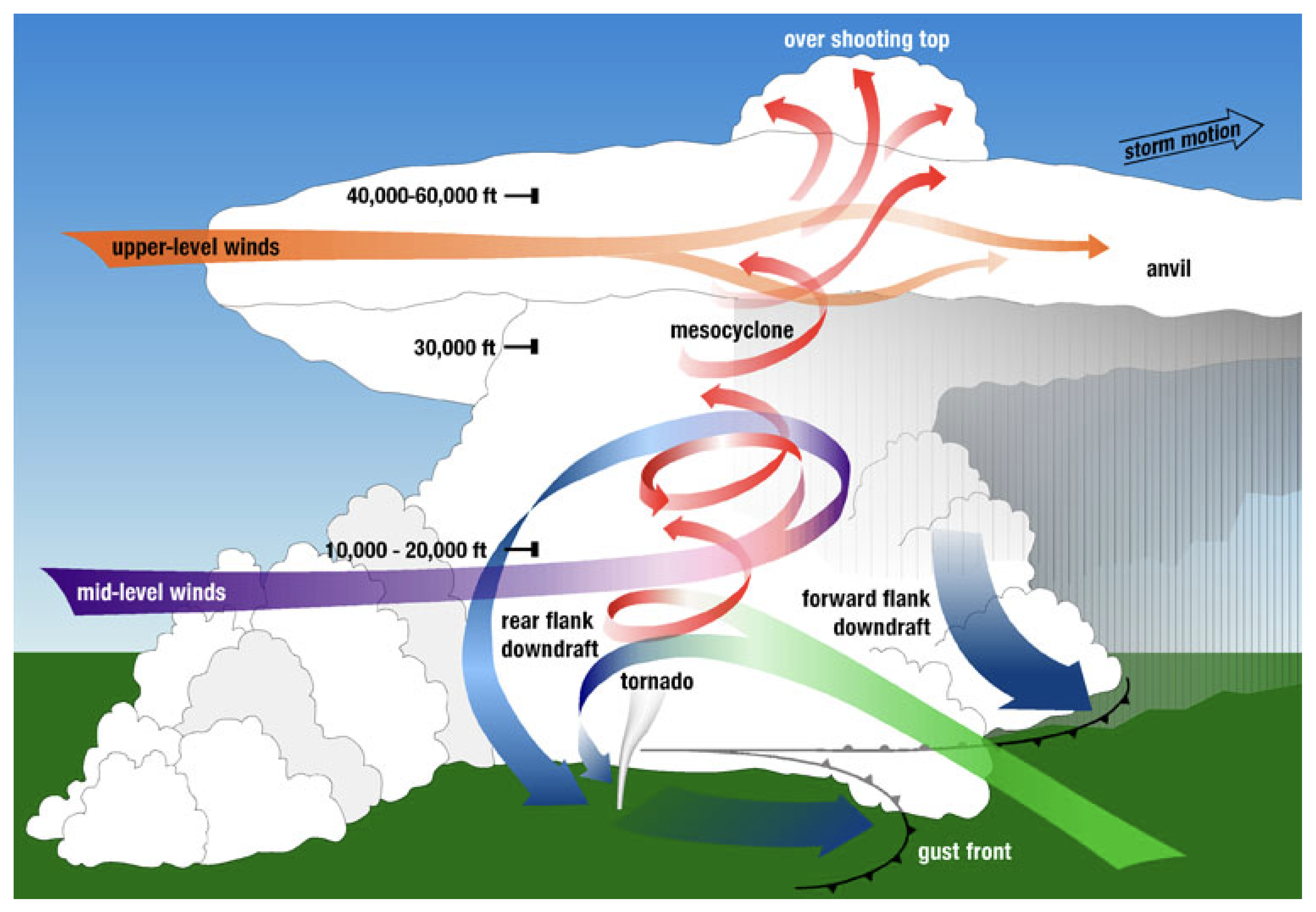
Figure 2.
Hairpin vortex model: vortex stretching (left) [1], vortex head lifting (center) [1], filaments and isosurfaces of rotation near the onset of furrows (right) [33].
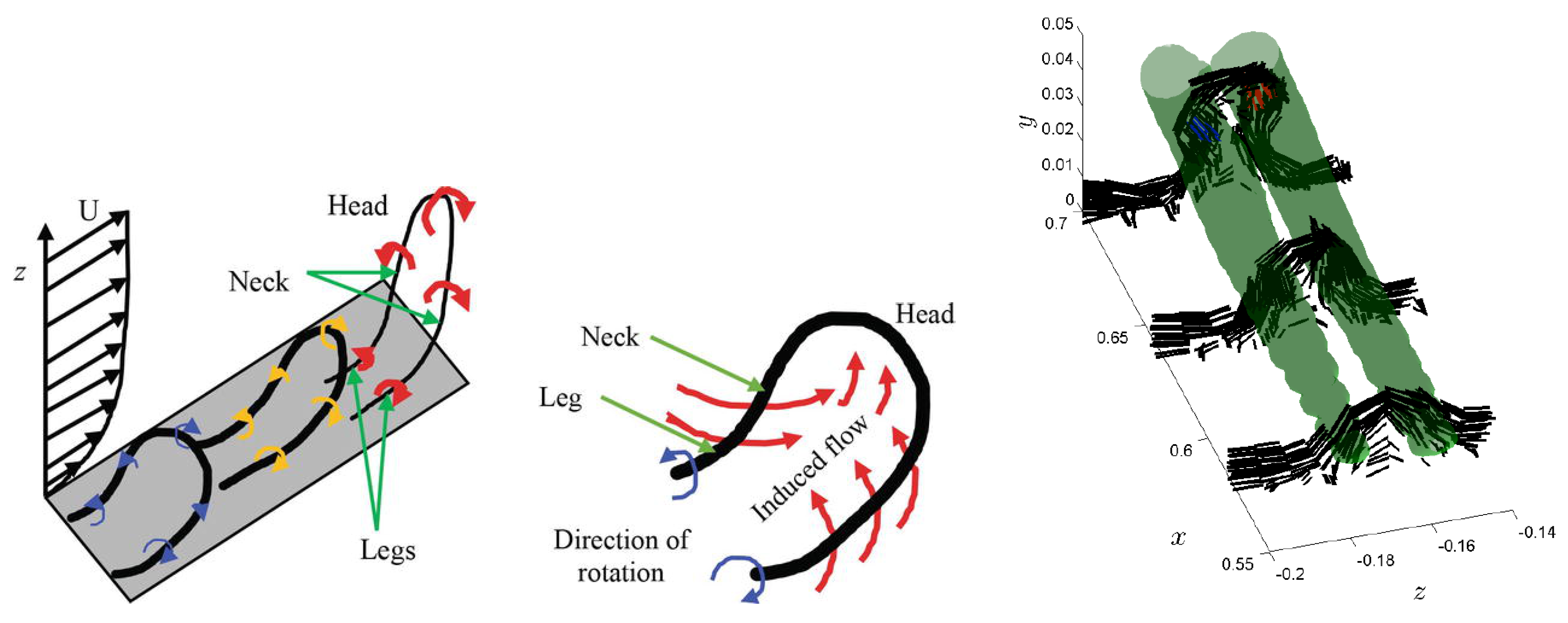
Figure 3.
Straight cusps between hairpin vortex legs, isosurfaces of rotation intersect the lobes of mushroom-shaped cusps (left); cusps at a fixed time showing progression to a turbulent flow at the end of transition (right) [33].
Figure 3.
Straight cusps between hairpin vortex legs, isosurfaces of rotation intersect the lobes of mushroom-shaped cusps (left); cusps at a fixed time showing progression to a turbulent flow at the end of transition (right) [33].
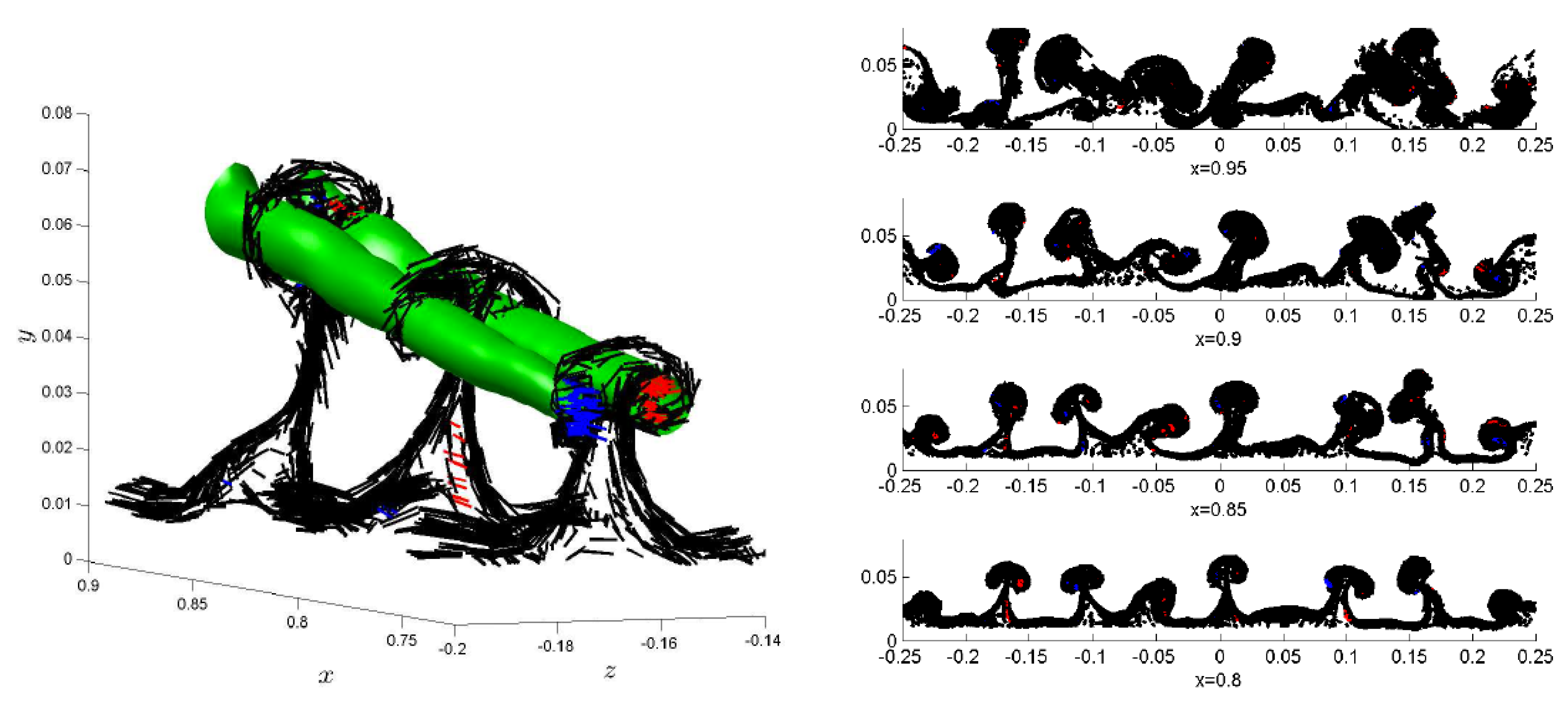
Figure 4.
Isosurface and near surface vortex lines, a continuum of which would form a corrugation (left) and cusps forming between counter-rotating vortices in coherent structures in the surface layer sampled (right) [16].
Figure 4.
Isosurface and near surface vortex lines, a continuum of which would form a corrugation (left) and cusps forming between counter-rotating vortices in coherent structures in the surface layer sampled (right) [16].
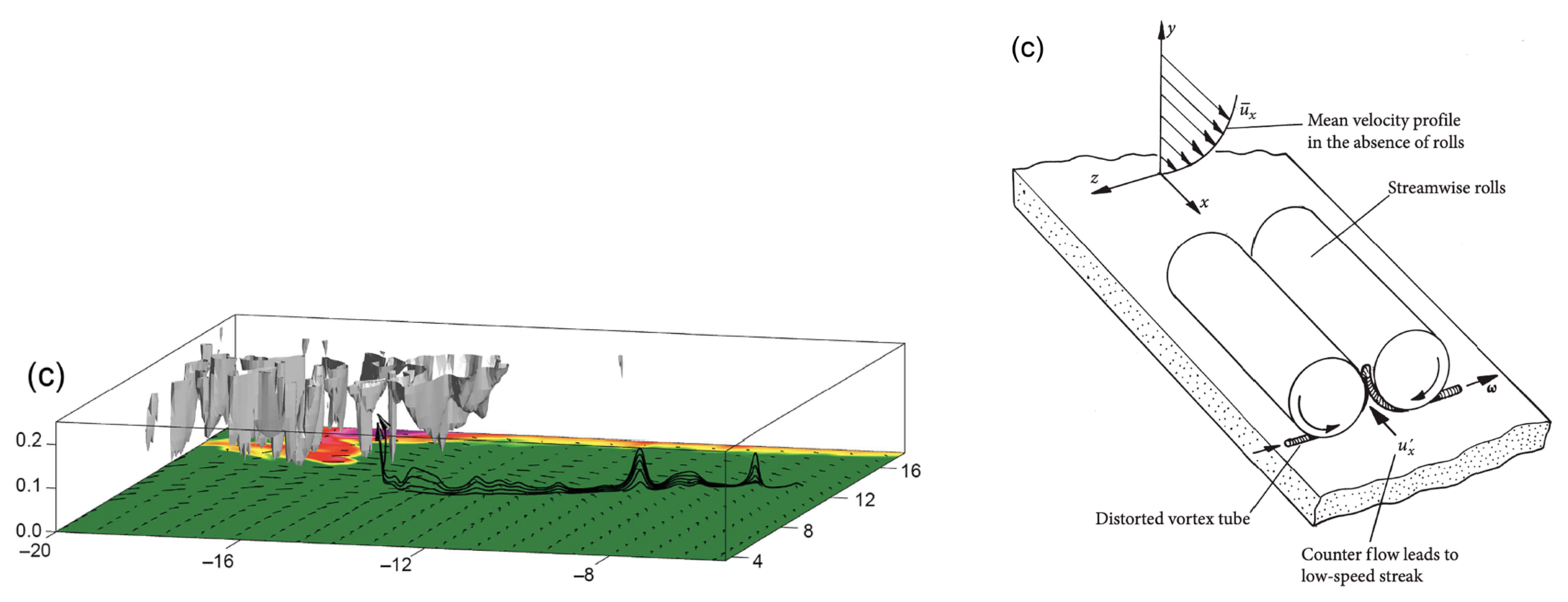
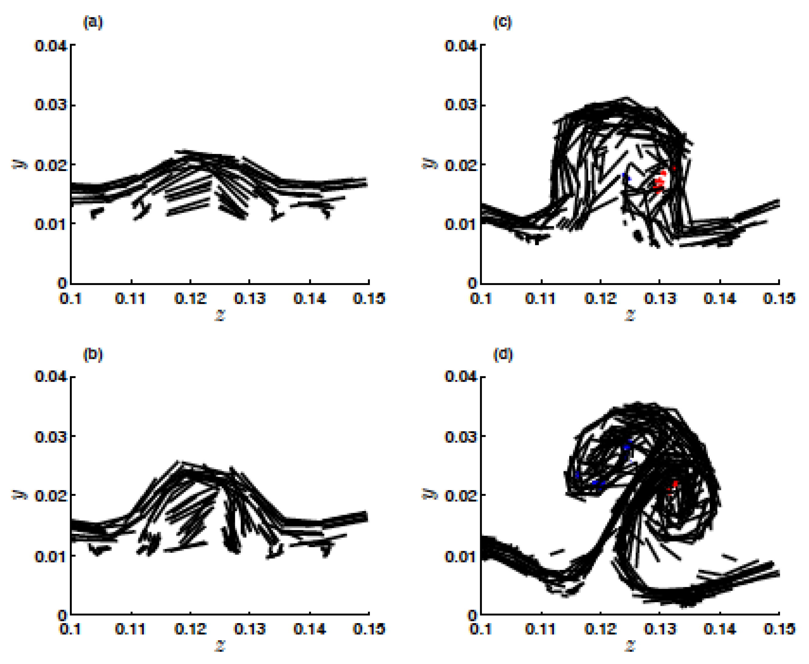
Figure 5.
Formation of vertical filaments: cusps in a furrow viewed by a moving observer [33].
Figure 5.
Formation of vertical filaments: cusps in a furrow viewed by a moving observer [33].
Disclaimer/Publisher’s Note: The statements, opinions and data contained in all publications are solely those of the individual author(s) and contributor(s) and not of MDPI and/or the editor(s). MDPI and/or the editor(s) disclaim responsibility for any injury to people or property resulting from any ideas, methods, instructions or products referred to in the content. |
© 2025 by the authors. Licensee MDPI, Basel, Switzerland. This article is an open access article distributed under the terms and conditions of the Creative Commons Attribution (CC BY) license (http://creativecommons.org/licenses/by/4.0/).
Copyright: This open access article is published under a Creative Commons CC BY 4.0 license, which permit the free download, distribution, and reuse, provided that the author and preprint are cited in any reuse.


