
Submitted:
31 July 2025
Posted:
01 August 2025
You are already at the latest version
Abstract
Dimensional tolerances and surface finish are two fundamental elements that must be carefully controlled during the manufacturing of industrial parts. The study of signals obtained from the machining of parts is useful for the control and monitoring of the process. For this reason, correlating these signals and information on the surface quality of the machined part is essential for the early detection of breaches in the quality levels of the parts. Therefore, the objective of this work is to develop an intelligent strategy capable of estimating the artificial geometric error induced in the part during machining. In order train these strategies, the experimental signals of the process and the three-dimensional scanned geometry of the machined part are used as starting data. This development aims to reduce both defects and production time, increasing the efficiency, productive capacity and environmental sustainability of the industrial process.
Keywords:
artificial intelligence
; milling
; 3D geometry
; scanning
1. Introduction
Industrial processes are constantly adapting to the needs imposed by the market. Currently, competition in the sector and the seek for sustainability in production processes have motivated the study and application of new methods that allow not only an increase in the profitability of the processes, but also a reduction in environmental impact. In machining processes, this translates into the need to exhaustively control the results obtained during the process. [1].
The main challenge in efficiently controlling machining processes lies in the variety of situations that arise, as well as in obtaining parameters and machine signals that provide valuable information on the quality of the operation.
The technological improvements developed in recent years, and the transition to industry 4.0, have allowed the deployment of increasingly precise sensors and with increasingly high sampling frequencies. This makes efficient data collection possible during production processes. The data obtained from these processes is extremely valuable since, if handled correctly, it can allow the identification of process anomalies or quality breaches during the process.
On the other hand, different software solutions have been developed that considerably ease the analysis and communication of information [2]. This has increased the exploration and deployment of data analysis and monitoring schemes. One of the most recently used tools are the different artificial intelligence (AI) algorithms. These techniques allow the analysis of complex data structures and the detection of patterns that are useful for industrial processes’ monitorization.
The main applications of AI strategies in machining processes can be classified into three groups according to their functionality:
Monitoring and predictive maintenance of machinery and tools: During chip removal processes, tools are subjected to varying wear conditions. Excessive tool wear or breakage directly impacts process performance. The analysis of data from historical operations facilitates the identification of failure patterns, thus allowing compliance with a predictive maintenance plan. For example, Achyuth, et al. (2018) [3] developed a strategy to monitor the tools’ condition by analyzing acoustic emissions captured during the process.
Optimization of cutting parameters: The optimization of cutting parameters during machining processes is critical to increase productivity and efficiency. Modeling the effect of these parameters is, therefore, of special interest for the industrial sector [4].
Analysis of defects (quality control): Lastly, one of the most common applications of data analysis, modeling and artificial intelligence in machining processes is based on the prediction of geometric errors that occur during the machining of parts. The deployment of this type of models allows real-time (in-process) quality control of the manufactured part, allowing the timely stop of the machine or the correction of the error. [5].
Defect analysis methods (quality control) are mostly based on training machine learning strategies. These are usually oriented to the generation of normality models of specific operations. For example, Eser, et al. (2021) [6], developed a predictive model of the roughness obtained after a milling process of an aluminum alloy. The roughness prediction is given by the analysis of parameters such as cutting speed, feed per tooth and depth of cut. In this way it is possible to predict the finish of the part based on the parameters selected for the operation.
Machining processes are high-precision operations. Therefore, it is essential to control the quality of the parts being produced in real time. In this way, the operation can be stopped in case the error exceeds the tolerable limit, thus increasing the productivity of the process. These geometric errors are the product of several reasons, such as errors in the clamping of the pieces, high operating temperatures, bending of slender tools or thin-walled pieces, vibrations, etc [7].
The objective of this article is to develop a geometric error prediction model for a milling operation based on both dynamometric signals and geometric data of the part obtained during the milling process and subsequent 3D scanning, respectively. In the document, first, the experimentation scheme is described, then the data processing methodology is analyzed and, finally, the obtained results are discussed.
2. Materials and Methods
2.1. Experimental Setup and Data Adquisition
In order to collect the necessary data to generate an error prediction model, the following processes have been carried out: (1) Raw flange scanning, (2) roughing operation, (3) Intermediate scanning, (4) Finishing operation and (5) Final scan of the piece. In Figure 1 Images of both the machining process and the scanner setup are shown.
In Figure 2, Scans of the part made at different stages of machining are shown using the assembly presented in Figure 1B). The part is a flange for the oil & gas industry.
This project focuses specifically on the milling finishing process of the frustoconical region of the flange. Specifically, it is a 5-axis milling. The tool used is a 25 mm diameter ball end mill with 2 cutting edges. The spindle rotation speed and feed rate are 3,200 rpm and 1,834 mm/min, respectively.
In order to obtain information on correctly and incorrectly machined areas, an artificial offset of 0.5 mm in the XY plane has been induced in the clamping of the part for the finishing operation. This eccentricity causes the generated forces to vary depending on the machined region. Therefore, expecting the AI strategy to be able to predict this geometric error that has been artificially induced in machining.
The data to be acquired for the training and application of an automatic learning strategy is divided into 2 groups: (a) Process / machine signals and (b) information on the geometric quality of the part.
The data acquisition of the process has been carried out using the SPIKE capture system from Promicron. From this system, different signals about the machining operation are obtained over a time domain, such as bending moments in the X and Y directions, axial force and torque.
In order to develop a process monitoring strategy, information on the geometric quality of the part is required. For this, a 3D scan of the piece after the finishing operation has been captured (Figure 2 C). From this scan, a cloud of points corresponding to the real part is recorded. The scanner has been mounted on a Fanuc robot and 8 capture positions have been set. The information obtained from the different captures of the piece has been unified through an automatic measurement program.
2.2. Data Processing Methodology
This project presents a methodology for data management in order to generate a model capable of detecting geometric errors during the milling process of the part in question.
The methodology of implementing artificial intelligence strategies and data analysis to industrial processes follows a structure divided into 5 main groups: (1) Pre-processing of the acquired data, (2) Study of variables, (3) Study of applicable AI models, (4) implementation of the models and validation, and (5) analysis and comparison of results (Figure 3).
2.2.1. Pre-Processing
At this stage of the project, the aim is to condition and standardize the captured data. Therefore, it is subdivided into conditioning and homogenization. The work carried out in each of these stages is detailed below.
The aim of data conditioning is to extract relevant information from the signals and filter the data obtained. The torque is recorded from the Spike capture system and the aim is to estimate the tangential force experienced by the tool. This force is calculated through the torque of the tool’s rotation axis. On the other hand, this signal is in time domain. To obtain the force in the spatial domain, the SPIKE and CAM signals have been synchronized.
Once the part is scanned after the milling operation, the point cloud obtained is adjusted to the theoretical geometry through the CAD. Subsequently, the geometric error committed at each point is calculated. This is calculated as the minimum distance between each point of the 3D scan and the closest point belonging to the CAD surface.
Thus, the tangential force and geometric error datasets are identical in structure. The first three columns are the X, Y, Z coordinates, respectively. The fourth column is the tangential force and the geometric error, respectively.
The points that correspond to the approach zone of the tool have been deleted from the dataset. This region does not provide relevant information, so its removal reduces the computational cost of training strategies without compromising their effectiveness.
In addition, the scan points that do not correspond to the region in which the machining forces are found have been filtered. This has been done by determining the spatial domain of the cutting data and removing all points from the scan that fall outside the mentioned domain in the Z coordinate.
To sum up, after this stage (data conditioning) two matrices are obtained that contain only relevant information on the machining process.
The objective of data homogenization is to homogenize the information to a single data structure. It is essential that the study parameters are calculated at the same points in order to estimate patterns and relationships between variables.
The information processed is not synchronized at this stage. That is to say, the points in which the geometric errors have been obtained do not coincide with the points in which the tangential force has been obtained. Therefore, it has been decided to work with the points of the CAM as a basis to be able to carry out this homogenization. For this, an algorithm based on KD trees has been developed, this structure allows to optimally solve the "nearest neighbor" problem [8].
Once the KD tree has been obtained with the 3D scan point cloud, the value of the geometric error has been approximated at each point of the dataset of tangential forces. This has been achieved by means of a weighted average of the geometric error computed with the three closest points. In addition, two conditions have been defined to mitigate information distortion. First, a search radius has been defined, and second, a minimum of three points has been established within said search region. For the geometric error approximation to be considered valid, both conditions must be met. If at least one is not met, then the information at that point is not "homogenized".
2.2.2. Study of Variables
The effectiveness of the different AI strategies lies fundamentally in the quality of the variables with which the model is fed. Therefore, the preprocessing stage is usually the most delicate in the process of implementing machine learning strategies. Usually, in this stage, not only is the information structured, but also the signal noise is filtered out. Such noise or spikes in the signals can significantly impair the performance of the strategies.
As previously mentioned, the data structure available up to this point has the following attributes
X coordinate
Y coordinate
Z coordinate
Tangential force
Geometric error
It may seem reasonable to feed the strategy with all the available parameters in order to obtain the best results. However, this stage has the objective of determining which parameters positively contribute to the model and discarding those that worsen the performance or application.
It is determined that it is essential not only that the strategy is precise and exact but also that it is applicable to a real case. The data with which the strategies are trained correspond to a particular scenario in which an eccentricity has been induced when clamping the piece in a specific direction of the XY plane and of a specific magnitude (0.5 mm). However, the strategy is expected to detect errors correctly in all directions and magnitudes.
2.2.3. Study of AI Models
There are numerous applications of AI strategies applied to similar problems in the literature. In order to select the most appropriate strategy, the objective of the model to be applied must first be correctly defined. In this case, the aim is to predict the geometric error committed based on the previously mentioned parameters.
The strategies that best adapt to the objective of the project are the regression algorithms. These allow to predict a continuous numeric variable based on the attributes (parameters) provided.
It is expected that the relationship between the geometric error and the selected parameters is not necessarily linear. For this reason, the algorithms to be applied must be able to work with non-linear or defined relationships. The SVR algorithm is commonly used for problems of this style. [9]. Therefore, it has been selected as a potential model for this project.
The results of the AI strategy will depend not only on the variables that have been used for the model but also on the hyperparameters of the algorithms. Hyperparameters are elements that can be modified in strategies and are not automatically optimized in the training stage. The main hyperparameter of the SVR model is the kernel.
SVR algorithms work by generating a hyperplane that fits the values of the dataset with which it has been trained. To obtain said hyperplane, the strategy uses a kernel. Consequently, the shape and quality of the hyperplane will depend substantially on said hyperparameter.
Kernels are functions that contain a series of operations that are executed in order to obtain the relationship between the variable to be predicted and the rest of the parameters. For example, when using a linear kernel, the strategy is conditioned to "force" a relationship between the variables that has the following form (Equation 1),
The most used kernels in SVR algorithms are:
Linear: (linear hyperplane, Equation 1).
Polynomials: conditions the shape of the hyperplane generated to polynomial equations of the degree that is specified
Radial basis function (RBF). Used to search for non-linear relationships.
In this project the following kernels will be evaluated: linear, polynomial (grade 2), polynomial (grade 3) and RBF.
3. Results and Discussion
For data management and implementation of the strategy, various modules of the Scikit-learn Python library have been used. In this library, not only the SVR algorithm is implemented, but also data management methods that have been useful for this project.
The results obtained both in the stage of the study of variables and in the implementation of the AI strategy are detailed below.
3.1. Variable Selection
As mentioned above it sounds reasonable to train the strategies directly with all the available parameters. However, as demonstrated below, this can be detrimental to the model.
It has been thought that by feeding the strategy with all the available variables, objectivity would be lost. Meaning by objectivity the ability of the algorithm to correctly operate with data with which it has not been trained.
Specifically, the proposed hypothesis is the following: The coordinates x, y, z condition the strategy directionally. Therefore, if the hypothesis is correct, it is expected that the generated model will not be able to correctly predict the error made when rotating the dataset. To test this, an algorithm has been trained with all the variables (x, y, z, Forces) and subsequently the validation dataset has been rotated 180º. For training, the SVR algorithm has been used with the 'rbf' kernel. Note that at this stage of the project the goal is not to judge the kernel but the variables.
Figure 4 A) shows the actual geometric error after rotating the data. It should be noted that all the dataset variables have been rotated together. Thus, the strategy should be able to correctly predict geometric errors.
Note that the strategy has been trained with the original dataset (not rotated).
As shown in Figure 4 B), the trained algorithm is not capable of correctly detecting the geometric error distribution in cases other than the training one. For this reason, it is concluded that the hypothesis is correct. By training the strategy with the x, y, z coordinates, a link is generated between the spatial and the geometric error. Preventing the error from being correctly predicted with a rotated dataset.
Consequently, it has been decided to carry out a transformation from Cartesian coordinates to cylindrical coordinates. Thus, the radius and theta angle are obtained as new attributes. The information provided by the radius does not condition the strategy as the Cartesian coordinates did. The same procedure has been carried out (rotate the dataset) and it has been confirmed that the strategy behaves correctly. However, it has been seen that when using the theta variable in the training stage, the result obtained is similar to that presented in the Figure 4 B).
Up to this point, the theta variable has been ruled out for the implementation of the algorithms. The remaining variables are the radius, the z coordinates and the forces. As shown in Figure 5, the radius and the z coordinates are closely related, it has been decided to eliminate the z coordinate since, like the x and y coordinates, it prevents the strategy from working correctly when displacing the dataset in the z axis.
Once this study has been carried out, it is decided that the variables to be used for training the model are the following:
Radius
Force
Geometric error (Predicted variable)
3.2. SVR Implementation
In order to evaluate the performance of the algorithms, a prediction error vector has been defined as follows:
So that is a vector that contains the prediction error committed in each of the validation points. The mean prediction error and its standard deviation are obtained from this vector. These two metrics allow quantifying the performance of each algorithm.
As previously mentioned, in the case of the SVR algorithm, the main hyperparameter to tune is the kernel. In Figure 6 the results of the validation of the strategy with the most relevant kernels are presented.
As can be seen, the best result has been obtained with the RBF kernel. The mean of the error committed by the prediction is 6.877 µm and the standard deviation 249.4 µm. The result is reasonably good considering that the deviation in the XY plane is 0.5 mm.
Regarding the accuracy, the means of the errors obtained were 5.36 µm, 31.2 µm, 28.1 µm and 6.87 µm for the linear kernel, polynomial of degree 2 and polynomial of degree 3, respectively. As seen, the RBF kernel is the second most accurate.
On the other hand, taking the RBF kernel as a reference, the standard deviations increase by 36.43 %, 41.23 % and 40.42 % for the linear, degree 2 polynomial and degree 3 polynomial kernel, respectively. In other words, the RBF kernel is undoubtedly the most accurate of the alternatives studied.
It has been observed that the RBF kernel is reliable throughout the different regions of the part. However, the prediction quality of the other kernels decreases as “higher” sections of the part are taken (higher z-coordinates)..
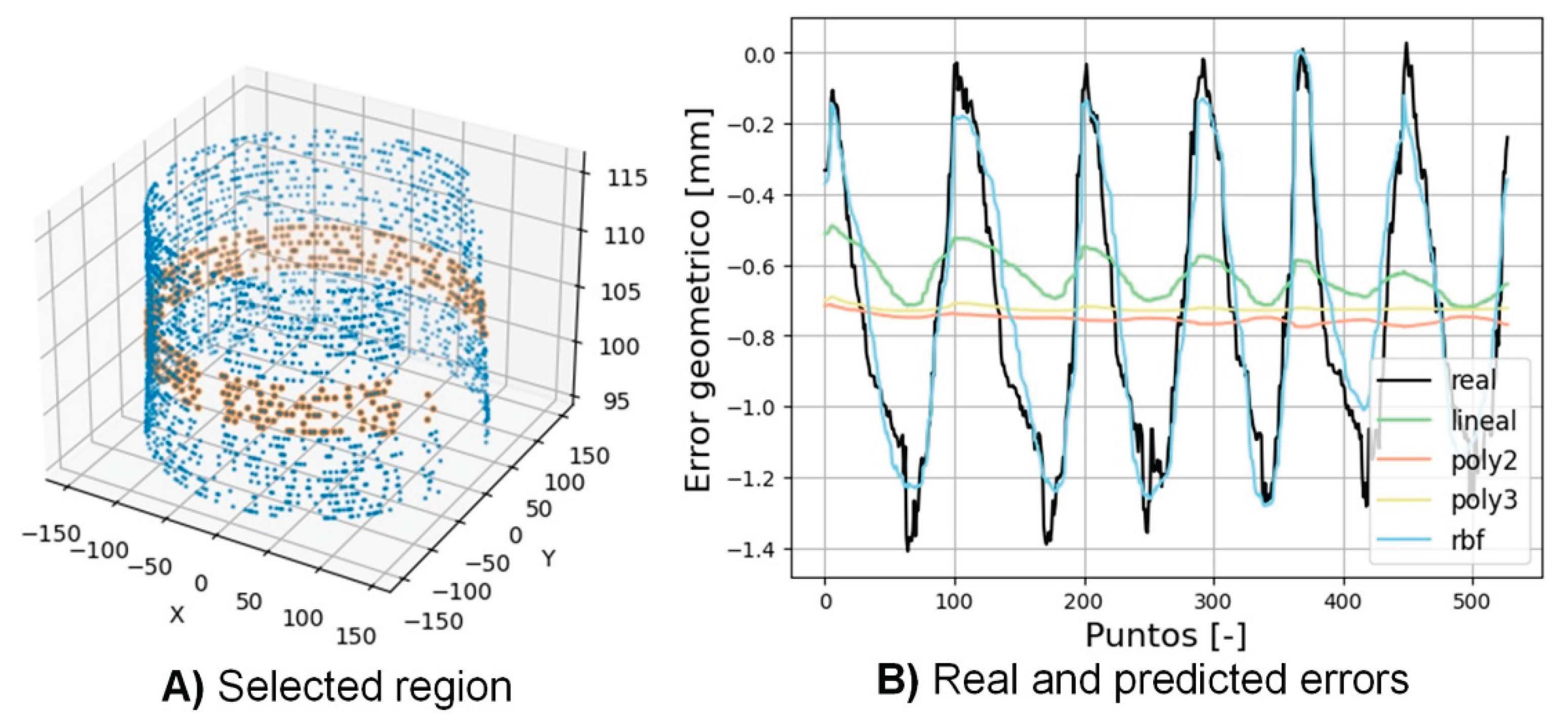
Figure 7 illustrates the quality of the predictions to observe the correlation visually. In this region it can be clearly seen how the RBF behaves better than the rest of the kernels. Obtaining mean square errors (MSE) of: 0.131, 0.151, 0.147 and 0.015 for the kernels: linear, polynomial (degree 2), polynomial (degree 3) and RBF respectively. Therefore, the predictions of this region agree with the general results presented in Figure 6.
When analyzing the complete domain of the signal, it is detected that the linear and polynomial kernels behave worse as the Z coordinate increases. This is due to the fact that the relationship between the variables analyzed is neither linear nor polynomial.
Finally, as previously commented, Figure 7 corroborates the results presented in Figure 6 and show that the rbf kernel is the most suitable for predicting the geometric error during the milling process.
This section may be divided by subheadings. It should provide a concise and precise description of the experimental results, their interpretation, as well as the experimental conclusions that can be drawn.
4. Conclusions
In this research, a prediction model has been developed that allows monitoring the geometric error of the part during the milling process. For this, machine sensors and 3D scans have been used.
It has been shown that the stages prior to the development of the AI strategy are essential to improve the objectivity of the data and guarantee an effective operation of the AI algorithm. In this sense, the Cartesian coordinates have been transformed to cylindrical and theta and z variables have been discarded.
The SVR algorithm based on the RBF kernel is the most accurate, reliable and precise strategy of those studied. On the one hand, other kernels (linear and polynomial 2 and 3) of the SVR algorithm have been studied. However, these increase the average dispersion by 40% over the RBF. On the other hand, the MSE of the predictions using the SVR algorithm with RBF in two chosen zones has values of 0.034 and 0.015, respectively, proving that the RBF prediction is consistent. Finally, in terms of accuracy, the mean error of the strategy is extremely low (6.877 µm). In summary, the SVR strategy with the RBF kernel has proven to be vastly superior in terms of accuracy and precision compared to the other strategies studied.
Finally, the feasibility of scanning as a technique for the supervision of industrial parts is demonstrated. In addition, this work demonstrates the potential of sensorization and artificial intelligence strategies in the control of machining processes.
Author Contributions
Conceptualization, Alain Gil-Del-Val; Data curation, Alain Gil-Del-Val, Rakel Pacheco Goñi, Meritxell Gómez and Ander Del Olmo Sanz; Formal analysis, Alain Gil-Del-Val; Funding acquisition, Alain Gil-Del-Val, Itxaso Cascón-Morán and Haizea González; Investigation, Alain Gil-Del-Val, Itxaso Cascón-Morán, Haizea González and Ander Del Olmo Sanz; Methodology, Alain Gil-Del-Val, Itxaso Cascón-Morán and Haizea González; Project administration, Alain Gil-Del-Val; Resources, Alain Gil-Del-Val; Software, Alain Gil-Del-Val and Rakel Pacheco Goñi; Supervision, Alain Gil-Del-Val, Rakel Pacheco Goñi, Itxaso Cascón-Morán, Haizea González, Meritxell Gómez and Ander Del Olmo Sanz; Validation, Alain Gil-Del-Val and Meritxell Gómez; Visualization, Alain Gil-Del-Val; Writing – original draft, Alain Gil-Del-Val; Writing – review & editing, Alain Gil-Del-Val, Itxaso Cascón-Morán and Haizea González.. All authors have read and agreed to the published version of the manuscript.
Funding
This research was funded by the Basque Government for financing the ECOVERSO project, ELKARTEK 2024 program (KK-2024/00095) and the ORLEGI project, ELKARTEK 2024 program (KK2024/00005) by the Grant European Commission, REINFORCE project, GRANT NUMBER: 101104204 URL: https://app.dimensions.ai/details/grant/grant.13717357.
Data Availability Statement
Not applicable.
Acknowledgments
the authors would like to thank the courtesy of ULMA Forged Solutions (ULMA Forged, S. Coop.) for having donated the industrial flange.
Conflicts of Interest
The authors declare no conflict of interest.
References
- Jamwal, A.; Agrawal, R.; Sharma, M.; Giallanza, A. Industry 4.0 Technologies for Manufacturing Sustainability: A Systematic Review and Future Research Directions. Applied Sciences 2021, vol. 11, 12.
- Yingfeng, Z.; Geng, Z.; Junqiang, W.; Shudong, S.; Shubin, S.; Teng, Y. Real-time information capturing and integration framework of the internet of manufacturing things. International Journal of Computer Integrated Manufacturing 2015, vol. 28, 8, pp. 811-822.
- Achyuth, K.; Sai P., N.; Rui, L. Application of audible sound signals for tool wear monitoring using machine learning techniques in end milling. The International Journal of Advanced Manufacturing Technology 2018, vol. 95, p. 3797–3808.
- Daniyan, I.; Tlhabadira, I.; Daramola, O.; Mpofu, K. Design and Optimization of Machining Parameters for Effective AISI P20 Removal Rate during Milling Operation. Procedia CIRP 2019, vol. 84, pp. 861-867.
- Dongdong, K.; Junjiang, Z.; Chaoqun, D.; Lixin, L. DongxingC. Bayesian linear regression for surface roughness prediction. Mechanical Systems and Signal Processing 20XX, vol. 142, 220.
- Eser, A.; Ayyıldız, E.; Ayyildiz, M.; Kara, F. Artificial Intelligence-Based Surface Roughness Estimation Modelling for Milling of AA6061 Alloy. Advances in Materials Science and Engineering 2021.
- W. Ge, L. Guangxian, P. Wencheng, R. Izamshah, W. Xu and D. Songlin, "A state-of-art review on chatter and geometric errors in thin-wall machining processes," Journal of Manufacturing Processes, vol. 68, pp. 454-480, 2021.
- M. Otair, "Approximate k-nearest neighbour based spatial clustering using k-d tree," CoRR, vol. abs/1303.1951, 2013.
- Author 1, A.; Author 2, B. Title of the chapter. In Book Title, 2nd ed.; Editor 1, A., Editor 2, B., Eds.; Publisher: Publisher Location, Country, 2007; Volume 3, pp. 154–196. [Google Scholar]
- Karimipour, S. A. Bagherzadeh, A. Taghipour, A. Abdollahi and M. R. Safaei, "A novel nonlinear regression model of SVR as a substitute for ANN to predict conductivity of MWCNT-CuO/water hybrid nanofluid based on empirical data," Physica A: Statistical Mechanics and its Applications, vol. 521, pp. Pages 89-97, 2019.
Figure 1.
Roughing process & 3D scanning.
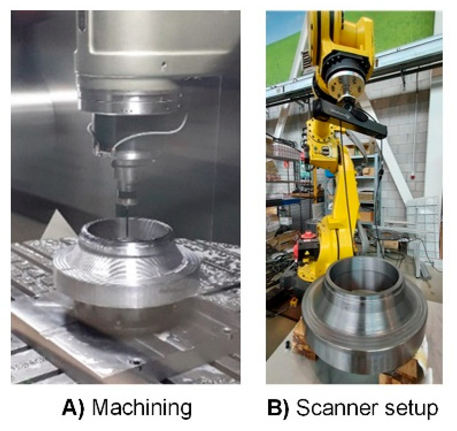
Figure 2.
3D scanning sequence.
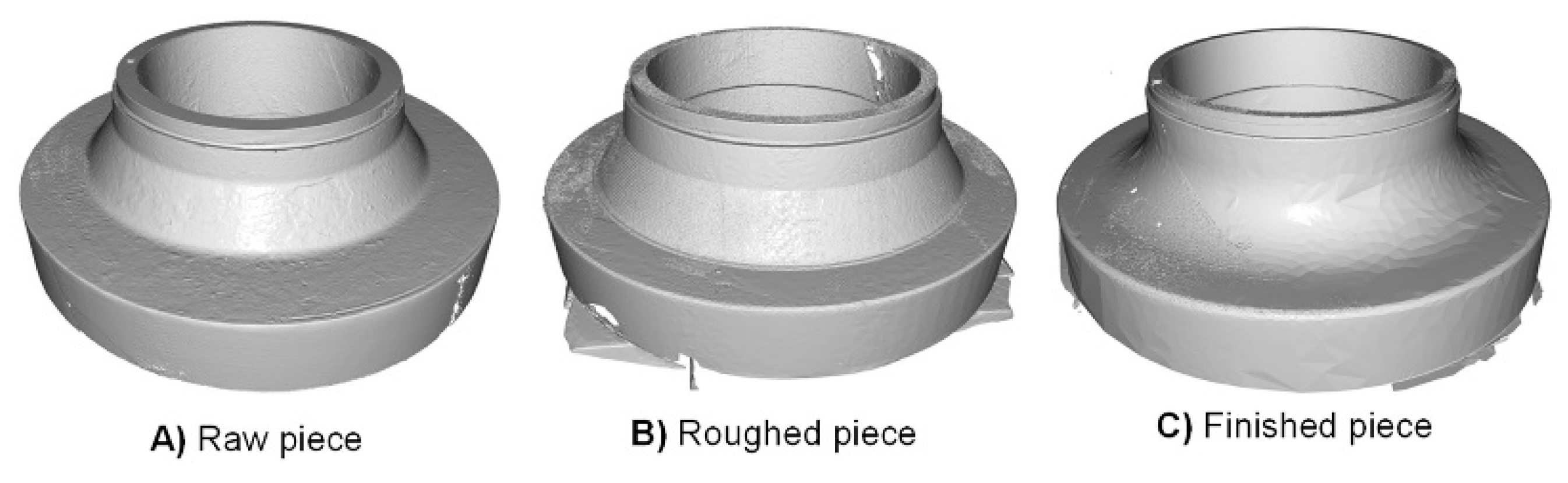
Figure 3.
Data processing methodology.
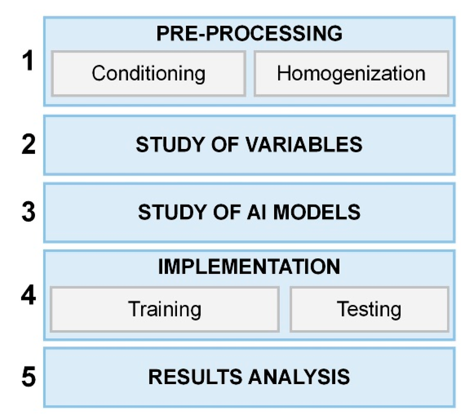
Figure 4.
Real and predicted errors after 180º rotation.
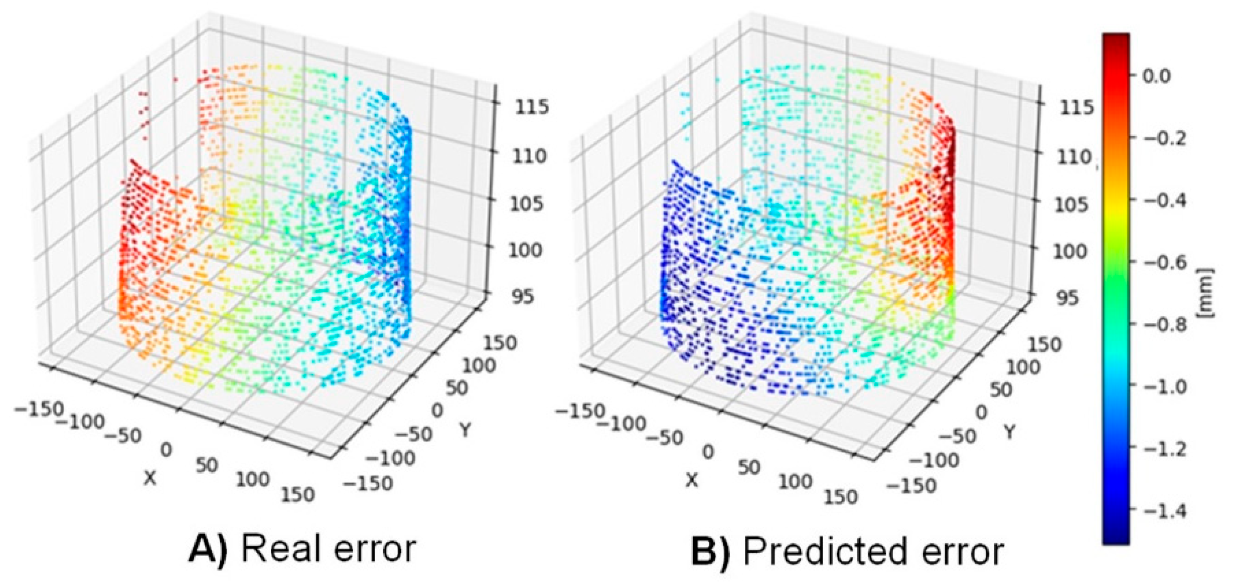
Figure 5.
Correlation matrix.
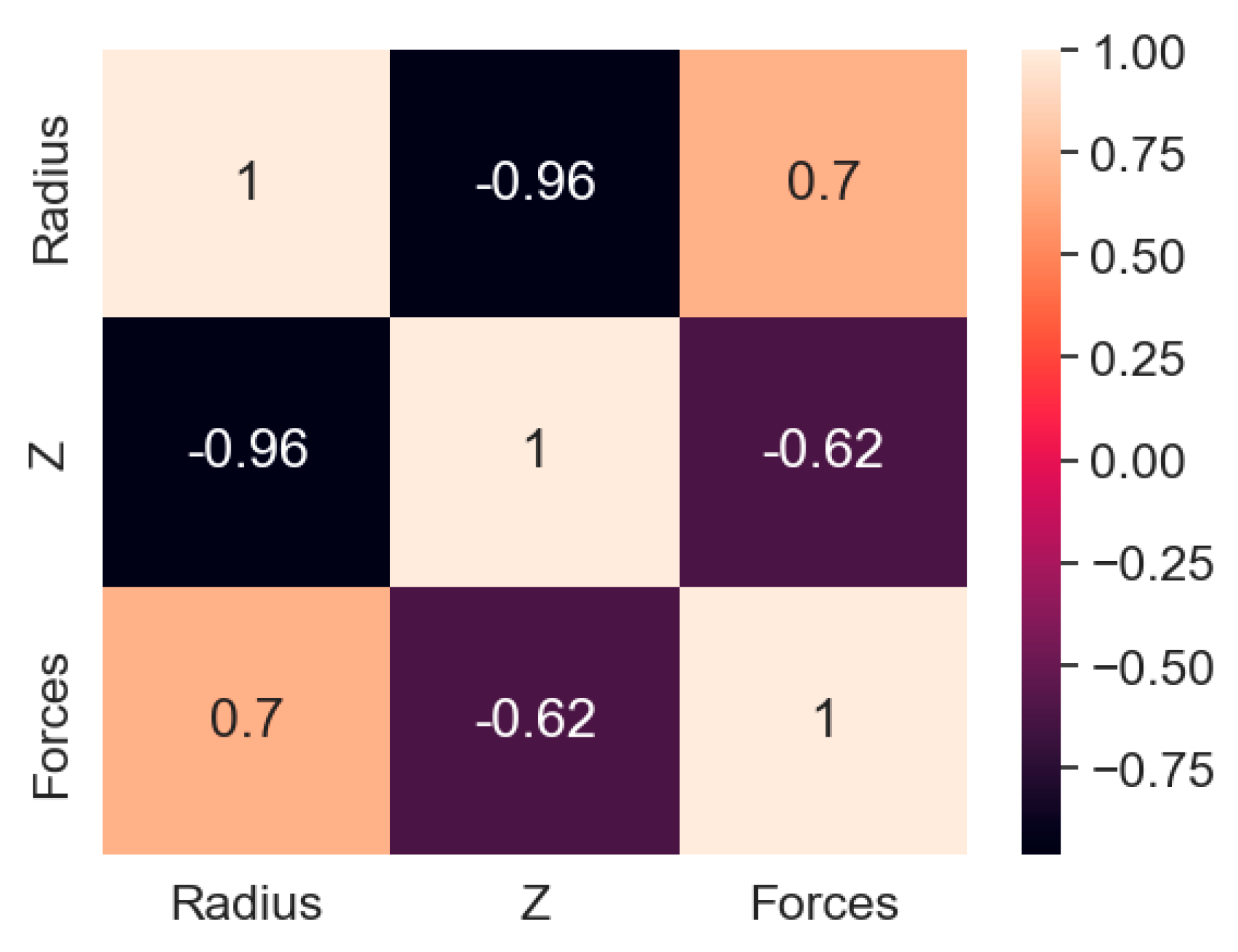
Figure 6.
Kernel comparison.
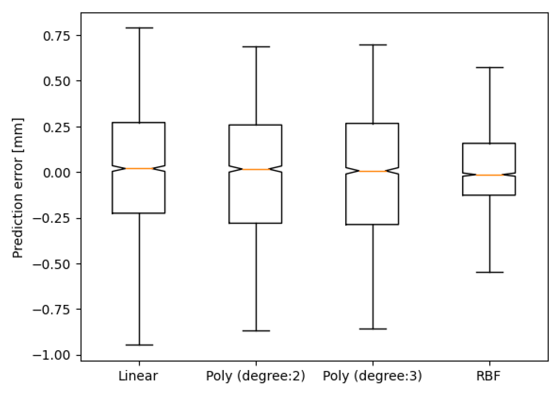
Figure 7.
Prediction comparisons.
Disclaimer/Publisher’s Note: The statements, opinions and data contained in all publications are solely those of the individual author(s) and contributor(s) and not of MDPI and/or the editor(s). MDPI and/or the editor(s) disclaim responsibility for any injury to people or property resulting from any ideas, methods, instructions or products referred to in the content. |
© 2025 by the authors. Licensee MDPI, Basel, Switzerland. This article is an open access article distributed under the terms and conditions of the Creative Commons Attribution (CC BY) license (http://creativecommons.org/licenses/by/4.0/).
Copyright: This open access article is published under a Creative Commons CC BY 4.0 license, which permit the free download, distribution, and reuse, provided that the author and preprint are cited in any reuse.


