
Submitted:
29 July 2025
Posted:
30 July 2025
You are already at the latest version
Abstract
The main aim of this paper is to describe the improvements to the enthalpy-based equation of state, and results of application to solid as well as porous lithium deuteride. In addition to being the lightest compound (which is an insulator at normal conditions), this material is an important component in devices employing thermonuclear fusion. The enthalpy-parameter versus pressure variation on five curves are used to provide an interpolation formula for its dependence on temperature. Then, a refined treatment of pore collapse, based on the $P-\alpha$ model and Menikoff's modification, is incorporated in the formalism, and checked with data on compaction of Cu powder. The enthalpy-based equation of state is applied to compute the Hugoniot of natural lithium deuteride (up to $10^3$ GPa pressure) and lithium-6 deuteride (up to $10^{6}$ GPa pressure). Comparison of predictions of the method with available data also includes porous cases up to initial density ratio of 1.78. The implementation of the equation of state in a hydrodynamic simulation code, which uses the flux-corrected-transport algorithm, is also briefly discussed. Simulation results for pressure versus fluid-velocity data show excellent agreement with those from Hugoniot experiments. Brief accounts of Vinet's zero-temperature isotherm, extended with that of the quantum statistical model, and the ion equation of state, which includes Debye-Einstein model, melting, rotation and vibration contributions of the molecule, and its dissociation are provided. Also, excellent new approximations to the electron equation of state contributions, based on Thomas-Fermi model are also discussed.
Keywords:
Equation-of-State
; Enthalpy-Based-EOS
; Lithium-Deuteride
; Hugoniot Shock-Propagation
; Computer-Simulation
1. Introduction
Equation of state (EOS) of materials is essential for the description of shock wave propagation [1]. The EOS defines a relation between pressure P, specific volume V and temperature T in a material in thermodynamic equilibrium [2], and it is generally formulated using V and T as independent variables [3]. The choice of independent variables is purely guided by convenience, in fact, the variables P and T are found more appropriate for describing hydrodynamic phenomena in porous and granular materials. This is mainly due to the ease in treatment of the shock induced compaction phase in these materials; it is particularly useful in dealing regions with multi-valued pressure versus volume variations. There have been significant progress in developing such EOS formulations for porous materials [4,5], which also have firm theoretical basis [6]. The choice of P and T variables is, perhaps, most appropriate for describing shock wave propagation in heterogeneous mixtures, as pressure P and material velocity relax quite fast to steady values after shock traversal, in comparison to thermal energy and hence temperature T[7]. Procedures to extract parameters of the EOS model (with variables) from Hugoniot data of solid as well as porous metals have also been attempted [8,9].
Authors of this paper pursued an approach for using P and T as independent variables via the enthalpy-based equation of state (EEOS) [10], starting from the thermodynamic definition of the enthalpy-parameter . This approach yielded the correct formulation for explicit accounting of contributions of electrons in EEOS [10]. It also yielded simple modeling of shock wave properties in solid and porous binary mixtures [11] and multi-component mixtures [12]. In addition, together with a suitable model for the fluid phase of the material, it was possible to evaluate the Hugoniot of highly porous Cu (porosity up to 10), whose final states are in the expanded volume region [13]. Furthermore, EEOS could be implemented within a solver for Euler equations of fluid flow [14]. This solver, which employs a second order accurate flux-corrected-transport algorithm (FCT) [15], provided pressure versus particle-velocity Hugoniot curves in excellent agreement with experimental data for different solid and porous materials. The present paper is mainly concerned with (i) introducing explicit temperature dependence in the enthalpy-parameter, (ii) correct implementation of compaction modeling in the model, (iii) a new set of formulas for thermal pressure and energy of electrons (based on Thomas-Fermi model), and (iv) applications to solid as well as porous lithium-6 deuteride (Li6D) and natural lithium deuteride (LiD-N). New schemes in the hydrodynamic simulations using the EEOS, to generate curves for solid and porous Li6D, are also discussed. The last item offers the possibility of prediction of data prior to experiments, as main details of the experimental setup could be implemented in numerical simulations.
The paper is organized as follows. In Section II, the general enthalpy-based EOS, together with temperature dependent is briefly discussed. The last feature follows from using versus P variations of different curves and then using a non-linear interpolation formula. This development also shows that there is no need to explicitly introduce electron contributions in the EEOS, as done earlier [10,13]; electronic effects need only to be introduced in the computation of curves. Modeling of the compaction phase and the modified model are covered in Section III. Applications and comparisons of the results of the model to LiD-N and Li6D are given in Section IV. Issues arising in the implementation of EEOS in the FCT solver for obtaining shock wave data (of Li6D), are covered in section V. Finally, Section VI summaries the work. The basic formulations of zero-temperature isotherm (Vinet EOS supplemented with quantum statistical model (QSM)), ion thermodynamic functions including Debye-Eintein model, melting, rotation and vibration contributions of LiD molecule, and its dissociation are given in the Appendix. Accurate new fits to Thomas-Fermi model functions for electron thermal pressure and energy, are also given there.
2. Enthalpy-Based EOS
Development of EEOS starts with the thermodynamic definitions of enthalpy-parameter and constant-pressure specific heat . These are given by and , respectively, where and E denote the specific enthalpy and internal energy, respectively. These parameters contain thermal contributions of ions and electrons, and so can be separated as , where and denote the ionic and electronic enthalpy parameters. Similarly, , where and represent the ionic and electronic specific heats, respectively. These separations are not absolutely essential in the formulation as shown below. Now, integration from 0 to T of the basic definitions yield
Here, is total enthalpy; the two terms in the sum represent zero-temperature and thermal contributions, respectively. The reference state parameters and , which refer to and given pressure P, arise as integration constants. Now, Equation (1) is rewritten as
where is introduced as an average enthalpy parameter. It should be noted that Equation (3) is exact and, importantly, it shows that should be temperature dependent in general. However, along a specific curve, T is expressible as a function of P by inverting the EOS: . Then , along that curve, reduces to a function of P only. It is denoted as with the subscript h indicating the specific curve. It should be emphasized that this argument holds only for along a specific curve like the isotherm, isentrope, principal Hugoniot, etc. By using the same arguments for , , and , where the subscripts denote ion and electron components, is expressible as a weighted average . But it is clear that is directly computed if the electron components are added in the functions and .
2.1. Specifications for EOS
A three component description, using the zero-temperature isotherm and energy , the ionic components of thermal energy and pressure and the electron components , is needed in any EOS specification [3,16]. These aspects are briefly discussed below, and in more detail in the Appendix.
The zero-temperature isotherm of Vinet et al [17,18] is known to be quite accurate up to about 1 TPa pressure [19], and is given by (see Appendix A.1). The volume is to be determined such that total pressure is GPa at ambient temperature (300 K) and volume . For very high pressures, energy and pressure must approach those of an electron gas around the nucleus, as given by the quantum statistical model (QSM) [20]. This model accounts for exchange and correlation effects in addition to electron density gradients [21]. Electron pressure in QSM is analytically expressed as (see Appendix A.1). An interpolation procedure [22] to smoothly go over from Vinet’s model to QSM uses a adjustable volume parameter such that the corrected pressure and for . These for smaller volumes are obtained by imposing continuity of and its first two derivatives at (see Appendix A.1). This procedure gives a smooth transition from Vinet’s model to the QSM [23], and is expected to be better than arbitrary modification of and at low volumes.
The thermal components of ionic energy and pressure (per gram) are expressed as and (see Appendix A.2). Here the original Jonson’s model for metals [24] is generalized so that the solid-energy consists of both the Debye ( acoustic modes) and Einstein ( optical modes) contributions [25]. Similar is the case for pressure . The components and (non-zero for , melting temperature) accounts for changes in specific heat upon melting and heat of fusion [16,24]. An additional term ( for ) is added to account for rotation, vibration and dissociation of LiD molecule. Three-term fits [26] to the Grüneisen parameters and are employed in the present model, and specific heat weighting provides the average (see Appendix A.3). The adequacy of these models are checked against experimental data on LID-N (natural) in the section dealing with results (see Section 4.1).
It is well known that electron thermal properties are provided by the finite-temperature TF model [27]. A new numerical method to solve the TF equation [28], and thereafter Brachman’s differential equation for electron energy [29,30], has been developed to generate extensive tables for and energy as a part of the present work (see Appendix A.4). The scaled variables and , where Z and R denote atomic number and cell radius, respectively, varied over and , in these tables. Thereafter, rational function approximations in the form and are derived, which have the correct low and high temperature limiting forms [28]. Dependence of and on cell radius is incorporated in the fitting parameters and , for (see Appendix A.4). Unlike the analytical fits available in the literature [31,32], these new expressions are more accurate and also applicable in expanded volume regions.
2.2. Temperature Dependent
The formulation of thermodynamic functions, outlined above, is appropriate for computing the parameters and along any arbitrary curve. As the expressions quoted are derivable from respective free energies, they provide consistent thermodynamic results. The constant-volume specific heat , Grüneisen parameter , and isothermal bulk modulus are readily determined on the specified curve. Temperature T on the curve is obtained by inverting the equation for given values of V and P. This inversion procedure for T is avoidable for the case of Hugoniot or isentrope, as T is determined by solving the temperature-equation [13] in an iterative manner (see Section 4 and Equation (10)). Then, the thermodynamic relations = = provide and isentropic bulk modulus . It is important to emphasis that all these quantities are obtained explicitly in terms of, say, V and T on the given curve, and the approximation that depends only on V is unnecessary. Finally, the defining relation, , provides the enthalpy parameter. Note that it also yields the equation = , which is useful whenever is available.
A simple scheme to generate solid Hugoniot is to employ the parameters C and S in the linear relation between shock speed and particle speed . Then the Rankine-Hugoniot jump conditions [1] provide volume on the Hugoniot explicitly as [14]
Here and are the initial pressure, volume and density. The parameter C is same as adiabatic sound speed ( bulk modulus ) while S is related to the pressure derivative of bulk modulus as . This equation is used to generate three and curves with the fixed parameters g/cm3, GPa, cm/s, which are appropriate to Li6D. The three curves in Figure 1 are obtained with the values (curve-1), (curve-2) and (curve-3). The other two (curve-0 and curve-H) correspond to zero-temperature isotherm and principal Hugoniot (S=1.11). The and curves corresponding the four cases (curves 1, 2, 3 and H) are also shown in the insets in this figure. The values of versus P obtained using the EOS model outlined above (see Appendix also) are shown in the main figure. Numerical fits of the data to the expression are shown as continuous lines in the figure. The fit constants are provided in Table 1 for all the five curves. The term in this expression is the limiting value of corresponding to mono-atomic ideal gas with . The fitting function is chosen so as to yield this limit for high pressures. The temperature data is fitted to the form ( K is ambient temperature). Table 1 also contains values of these fitting constants.
The formulas for and are used to develop an interpolation scheme for computing . First of all, note that in the vicinity of any of the five curves, the expression , where is its value at , provides a temperature variation. This function tends to the asymptotic limit as . The choice of the function ensures that reduces to on the curve-h. Thus the interpolation tends to as as well. Now the function is generalized to the Lagrange polynomial, viz. and is expressed as
On any of the five curves, say curve-h, the parameter reduces to and hence would yield the fitted function .
3. Modeling Compaction Phase
A parameter that is used to characterize porous materials is its initial porosity, defined as , where and are, respectively, the initial specific volumes of the porous and the solid materials. Carroll and Holt [33] considered the compaction of a spherical pore, surrounded by an in-compressible matrix material, due to an applied time-dependent pressure P on the outer surface of the matrix. Time dependence of P is characterized by the linear ramp rate . These authors derived a formula for the variation of porosity function with pressure, and it is expressed as for and for . Here, Y is the strength of the matrix material and is the elastic critical pressure of the porous material. Compaction process is initiated when P exceeds . This formula agrees well with numerical results of the collapse model. Their analysis also explained the validity of the relation , where V and represents the specific volumes of the porous and matrix materials. However, it is found that there are some differences between numerical results for pressure P in the porous material and those provided by the model formula, viz. , for . This relation is also expressed as , where and represent thermal energy in the porous and matrix materials, respectively. Thus the range of validity of the relation , , is found to be much more than that of . Another assumption in the model is that the zero-temperature energy is unaltered due to the presence of pores, but pressure increases during the compaction process. As the solid matrix is assumed to be in-compressible during compaction, is the same as . So, a simple way to extend Equation (1) to porous materials is to compute from Carol-Holt relation for a specified value of P and obtain the zero-temperature volume for porous material as . A more accurate approach is discussed next.
3.1. Low Pressure Compaction
First step in this detailed approach to model compaction process is to rewrite Equation (1) for the matrix material as
Here the definitions and are used. The subscript m in , and denotes that these variables pertain to the solid matrix. Note that Equation (7) is the isotherm of the solid matrix. Now, using the relations , and yields the equation
Starting with a specified value of P, and Carol-Holt formula for , Equation (8) provides the isotherm of the porous material. All the aspects of the model are present in this equation. A similar equation, however, using an approximate Mie-Grüneisen relation (which assumes is a constant), has been derived elsewhere [34]. But Equation (8) is more general because accurate expressions for and of the solid matrix can be employed. The advantage of using P and T as independent variables is most evident in obtaining Equation (8) for porous materials.
The compaction curve along the Hugoniot follows by substituting the Hugoniot equation for energy, into Equation (8) (see also Equation (9) in Section 4). Results obtained in this manner at 300 K and experimental data [35] on porous Cu are compared in Figure 2. Excellent agreement obtained establishes the accuracy of Equation (8). Since temperature involved is very low, (P) along the zero-temperature isotherm of Vinet et al is used for the computations. It is verified that the isotherm of Li et al [36] also produces indistinguishable results. All the data needed for Cu are tabulated in the Appendix (see Table A1 and Table A2) .
3.2. Menikoff’s Modified Model
The assumption of model that internal energy does not change during compaction is thermodynamically inconsistent. The modification proposed by Menikoff [37] starts with the Helmholtz free energy model of the porous material . Here is the free energy of the solid matrix and is its volume fraction at an intermediate compaction; being the initial volume fraction. The term , arising purely due to the pores, in the expression for free energy may be related to the surface energy of pores as , so that is an increasing function of and it vanishes at . In general, is an independent variable characterizing the porous state, and hence pressure in the porous material is , which is the basic equation of model. Internal energy of the porous material is , as entropy is the same as that of the solid matrix.
Now, if the material relaxes very fast to equilibrium conditions after attaining pressure P and temperature T, then the volume fraction also corresponds to equilibrium conditions, and can be denoted as . It should be determined from the condition (i.e., should correspond to minimum of F). This yields the relation , which implies a relationship of the form at equilibrium conditions, where is a suitable, usually empirical, function. Note that in Carroll-Holt model, (or ) corresponds to a time-dependent pressure P, and is dependent only on . However, volume at equilibrium, (in is determined in terms of (and T) via the EOS of the solid matrix. The differential equation is integrated starting form to obtain . The Carroll-Holt compaction function is rewritten as for . The assumption that this is also valid in equilibrium condition, yields the differential equation . As the matrix material is in-compressible during compaction [33], . This reduces the equation for purely in terms of matrix material constants. Thus the improved model also provides changes in internal energy during compaction, thereby removing the inconsistency. The differential equation is integrated along the low pressure compaction curve of Cu considered earlier (see Section 3.1). The variation of versus P (as is related to and hence P) is shown in in the inset figure of Figure 2. Energy on the Hugoniot at 2.5 GPa is found to be , so the value of , seen from the inset figure at the same pressure, is negligible. Thus, the original model (within its range of validity) is adequate for all practical applications.
4. Application to Lithium Deuteride
Substitution of the expression for energy along the Hugoniot, , into Equation (8) yields the volume-pressure curve (on the Hugoniot)
where . Similarly, . The subscript m on and indicates that these quantities should be computed at pressure in the matrix material. Thus, note that and contain the parameter in their present definitions. In the equations used by earlier authors [4,5,13], the parameter appears only as . Thus, quantities like , , etc. occurring in Equation (9) were computed at P in those papers, and not at . Of course, the differences in above equation are significant only for higher porosity, like , and in the compaction phase. Nevertheless, it should be noted that Equations (8) and (9) follow from correct application of the theory. It is not straight forward to implement this model when V and T are treated as independent variables. For high values of P, Equation (9) shows that as the parameters and . Note that this is just the mono-atomic ideal gas limit as .
Volume in Equation (9) is determined together with an equation for temperature T on the Hugoniot, as depends explicitly on T. The differential equation for T is [14]
Here is the constant-pressure specific heat, at pressure , of the matrix material. Using a forward finite difference scheme, a discrete form of Equation (10) is obtained as
Here the subscript k on different variables denotes their respective values at where is an increment in pressure, and . Finally, note that Equations (9) and (11) are evaluated iteratively at each to obtain . Starting with a guess value of , say , one iteration is complete on obtaining , using Equation (9), and then updating , via Equation (11). These steps are repeated until values of converge within a prescribed error (say, ). Centered values of parameters in Equation (11) are introduced after first iteration, which converge in few (3-4) steps. Completion of the whole process for , provides volume and temperature along the Hugoniot in a consistent manner. The method is applied to (natural) LiD and and compared with experimental data below.
4.1. Isotherms of Natural LiD
Before considering shock wave data on (natural) LiD-N, the ion model and zero-temperature isotherms (discussed in Appendix) are evaluated using experimental data. Employing in situ high-pressure and high-temperature neutron diffraction techniques (for pressures up to 4.1 GPa and temperatures 1280 K), thermodynamic properties of LiD-N () are available in the literature [38]. Analysis of the pressure-volume data at 300 K, using the finite-strain EOS , where and , authors of this work deduced GPa assuming that with . Similar analysis of the data at 500 K shows that GPa [38]. These data are re-interpreted in the present paper using the zero-temperature isotherm of Vinet et al [17,18] (see Appendix A.1). It is known [39] that this is an excellent model for LiD-N (see the inset in Figure 3). Einstein-Debye model, which takes into account the optical and acoustic branches of lattice vibrations (see Appendix A.2), is used as the thermal model. The results so obtained for the two isotherms of LiD-N are compared with experimental data [38] in Figure 3. Solid lines are from present computations while symbols denote experimental data. Agreement to the data at 500 K needs explicit accounting of optical branch while the acoustic branch alone is found adequate for 300 K data. The parameters used for all calculations are listed in the Appendix (see Table A1 and Table A2).
4.2. Principal Hugoniot of natural LiD
A series of shock wave experiments driven by impact with velocities in the range km/s are reported on single crystals of LiD-N with initial density around [40]. Pressure versus volume on the principal Hugoniot (up to 570 GPa) and behind re-shock states (up to 920 GPa) are available for comparison with results of EEOS formalism. These results significantly extend those of earlier LASL shock wave experimental data (up to 45 GPa) (see Section 4.3) available in the literature [41]. Results of computations are shown in Figure 4, and compared with both sets of data (filled circles and filled stars for high and low pressures, respectively). Excellent comparison shows the accuracy of the EEOS model up to pressures of about 600 GPa. The agreement between computed results and data is similar to that obtained via ab-initio molecular dynamic (AIMD) calculations [40]. The inset graph in Figure 4 shows computed temperatures on the principal Hugoniot versus pressure and experimental data (filled circles). To account for the contribution of dissociation of LiD molecule to ionic energy, a term of the form , with , is added so that the total ionic energy is (per LiD molecule) in the high temperature limit (see Appendix A.2). Although there are only four data points, the agreement with the results of EEOS is satisfactory.
Next, the results of EEOS model are compared with experimental data [40] on re-shock Hugoniot of LiD-N. The same formula in Equation (9), with initial conditions on the principal Hugoniot, generates the re-shock states. The first-shock and re-shock states (filled circles), shown in Figure 5, agree well with computed results (continuous lines). This comparison further affirms the accuracy of the model up to about 900 GPa. Note that higher densities (and lower temperatures), in comparison to that on the principal Hugoniot, are obtained on the re-shock states.
4.3. Solid and Porous Hugoniot
Extensive compilation of results of shock wave experiments from LASL, for a variety of solid and porous materials, are available [41]. These data are primarily based on measurements of fluid velocity , shock velocity and free surface velocity . Many materials follow a linear relation beyond the elastic pressure regime (see Table A1). Tables of P versus V, deduced from measurements, in the data files are directly comparable with computed results shown in Figure 6. Data considered for comparison correspond to solid LiD-N , solid and two porous cases of (with initial porosity and , respectively) (see the legends in the figure). Successive graphs in this figure are shifted upwards by 10 units for clarity. There is good agreement between computed results and the data. Similar comparison is also found for other porosity values 1.052, 1.081, 1.379 and 1.568.
The increase in pressure P due to increase in the initial volume is clearly evident from these results. The Hugoniot relations [1], which imply , show that P increases with for the same shock wave energy density and final volume V. This feature is also clear from the results of solid LiD-N and . But, shock compression of porous materials involves initial compaction, leading to pore closure, followed by compression of the matrix material [34]. The microscopic mechanisms involved during the process of pore collapse are: (i) initial shock loading of solid matrix, (ii) shock break out at the pore interfaces, (iii) collision energy dissipation of the ejecta, and (iv) consequent local heating. Thus, higher temperatures and pressures are produced on shock loading of porous materials [10]. Furthermore, there is anomalous expansion in the shocked state, for higher initial porosity. For instance, when initial porosity of Cu is more than 2, the final volume increases with pressure, instead of decreasing. Then P taken as a function of V becomes double valued. In this situation, the choice of P and T as independent variables in thermodynamic modeling, and hence EEOS, becomes preferable.
Next, Hugoniot of at extreme pressures (up to GPa) is considered, where multi-valued pressure versus volume arises. Results of extensive computations of the principal Hugoniot of up to pressures about GPa is reported [42]. These authors used the Khon-Sham density-functional molecular dynamics (KSMD) for temperatures in the range 0.5 to 25 eV, and extended it with orbital-free density-functional molecular dynamics (OFMD) up to about eV. The OFMD scheme is based on Thomas-Fermi-Dirac model. Both methods are matched in the intermediate range of 10 to 20 eV. Detailed results for pressure P and temperature T versus density on the principal Hugoniot of the solid (), and P versus data for 4 porous-cases () are provided.
The results computed using EEOS together with data obtained via KSMD (filled stars for P > 100 GPa) and OFMD (filled circles) for solid are shown in Figure 7. LASL experimental data [41] up to 45 GPa (filled stars) are also shown. Initial build up followed by exponential increase (note the Log-scale) and thereafter bending to lower densities are the characteristic features of the curve. The bending, and consequent double-valued pressures, is due to ions and electrons in approaching the behavior of ideal fluids. Maximum compression achieved is just which may be compared with 4 for mono-atomic ideal gas. This increase arises from absorption of energy from the shock for dissociation of molecule and thermal ionization. At the extreme limit of pressure, GPa, the shocked state would contain ions of Li6, D and electrons. Almost all features of the complete Hugoniot are brought out by the EEOS model. Temperature T along the Hugoniot is compared with KSMD (filled stars) and OFMD (filled circles) data in the inset figure. Although there are some differences, main features of curve, particularly temperature K reached at maximum compression , and bending of the curve are reproduced by EEOS model.
Finally, the results based on OFMD scheme for solid and four porous cases are compared with those of EEOS model in Figure 8. The comparison is similar to that of pure solid case. As intial density decreases from , maximum density reached decreases, although compression factor remain the same. For the case of maximum density reached is .
5. Implementation of EEOS in Euler Solver
The Euler equations describing the conservation laws of fluid flow are non-linear partial differential equations, in and time t, for density , fluid velocity and total energy . These are expressible in a fixed (Eulerian) reference frame or a moving (Lagrangian) frame [1]. For the cases of all one-dimensional geometries (planar, cylindrical and spherical) the integral form of general conservation law is written as:
Here, is the time-dependent volume element (arising due to moving grid in Lagrangian frame) and its surface element. The spatial coordinate is r, and u and represent the fluid velocity and grid velocity along the r-coordinate. The grid velocity assumes values 0 and u in Eulerian and Lagrangian schemes, respectively. Volume and surface elements in one-dimension are: and , respectively. The index n takes values 1, 2 and 3 in planar, cylindrical, and spherical geometry, respectively. Here, G stands for , or corresponding to the three Euler equations for mass, momentum and total energy [1]. The internal source function (third term in Equation (12)) is explicitly written in terms of coefficients B, C and D. Note that for the energy equation, but zero for mass and momentum equations. Similarly, and for the momentum equation, but these are zero for the other two cases. These and source rate Q are functions of r and t. An EOS which provides pressure in either form or is required to close the system of equations. It is sufficient to have an algorithm to treat Equation (12) for solving Euler equations in the order . In fact, this form is much more general and a large class of problems is mapped into it by defining the coefficients appropriately.
The one dimensional FCT algorithm, developed by Boris, Book and co-workers [15], solves a system of conservation equations. This algorithm consists of a convective diffusive stage which is followed by an anti-diffusive stage. The fluid variables are updated using a three point spatial difference scheme during the former stage in every time step. Some amount of diffusive transport is allowed in this stage so that numerical stability and positivity are preserved. However, the latter stage of the algorithm involves addition of anti-diffusion fluxes for reducing the smearing effects of diffusion. The important aspect of the method is that the anti-diffusion fluxes are corrected such that no new overshoots in fluid variables are generated. Integration in time is improved using a two-step scheme wherein time-centered source terms are generated before the full time-step integration. The FCT algorithm is coded as FORTRAN subroutines [15] which are easily used with a driver program and an EOS package. The algorithm has the flexibility that either the Eulerian scheme or moving Lagrangian scheme is used in the simulation. The method is also discussed in detail, and applied to simulate several strong-shock problem [43], and the results so obtained are found to be quite satisfactory. Next, the updating equations for P and T, while using EEOS, are discussed.
5.1. Updating P and T
After every hydrodynamic sweep (in time), spatial profiles of P and T in the meshes are to be updated. The information available from the FCT algorithm for this purpose are the increments or and at all meshes. Assumption of local thermodynamic equilibrium yields the relations
Here, Equation (13) follows by considering (as in EEOS) and the definition of iso-thermal bulk modulus. A basic relation involving Grüneisen parameter , and , viz. , is also employed. Similarly, Equation () arises by taking and using the definition . This equation can be rewritten using the `TdS’ relation (which assumes energy conservation and reversible changes), and also Equation (13). The resulting matrix equation, which provides and is given by
The vector on the RHS comes from the hydrodynamic cycle. All the terms (like , , , etc.) occurring in the matrix elements are readily computed using the variables , , available at the beginning of the cycle. The EEOS model provides in term of the known values of and . After solving the system, and provide estimates of P and T at the end of the cycle. Another iteration, after updating the matrix elements as averages of beginning and end values, is done to obtain a time-centered algorithm.
A root-finding method [14] to determine and is feasible by rewriting Equations (8) and (13) as
Here and are provided from hydrodynamic cycle. Further, , and and denote averages of beginning and end values. Starting with , first Equation (16) is solved via root-finding method to get . Thereafter Equation () directly provides . A second iteration is done to redefine other parameters as centered values, as explained earlier.
5.2. Shock Pressure Versus Fluid Velocity in
As an application of EEOS package in FCT solver, a configuration of slabs, similar to that used in impact experiments, is considered next. In impact experiments, a projectile (also called impactor) impacts on a target plate and launches two shock waves, one into the plate and the other back to the projectile. After an initial acceleration, fluid particles in the target attain a constant velocity, called fluid (or particle) velocity . The shock wave moves in the target with its own velocity denoted as shock velocity . Measurement of and in a series of impact experiments provide the principal Hugoniot of the target material.
Simulations in used a configuration consisting of 5 mm thick target, impacted with 3 mm thick impactor. Impact velocities used are up to about 12 km/s. In the first set of simulations, both the impactor and target are chosen as solid (density ), because inelastic collision between them (same material) yields a fluid velocity which is half of the impact velocity. At time , all the mesh-interfaces in the impactor are assigned the impact velocity. Meshes of width and time steps of are used in each calculation. The resulting hydrodynamic motion in the target is followed up to about 100 , thereby yielding steady values of pressure and fluid velocity in a single simulation. A series of such simulations provide the P versus Hugoniot shown in Figure 9 (curve-1), which is compared with the LASL experimental data (symbols) [41]. Excellent agreement obtained with experimental data demonstrates the adequacy of EEOS and its integration with the FCT code. The same procedure is then repeated with targets of two initial porosity specified via . The results obtained (curve-2) and (curve-3), respectively, for and , are also compared with experimental data in Figure 9. Good agreement is found in these cases as well. It should be noted that there is significant attenuation of the shock wave in porous targets, and so P and values have to be picked up, from the simulation data, from meshes close to the impactor-target interface.
6. Summary
The main aim in this paper is to provide a consolidated account of the different aspects of the generalized enthalpy-based EOS. Utility of this scheme (which uses as independent variables) over the conventional approach (with as independent variables), in dealing with multi-valued P versus V variations is brought out. Several new ideas such as: (i) an average temperature-dependent enthalpy parameter (see Equation ()), (ii) explicit interpolation formula for (see Equation (6)), (iii) correct use of the model for treating compaction (see Equation (8)), and (iv) updating P and T in the EEOS implementation in the FCT solver for Euler equations (see Section 5.1), are discussed. Results of applications to solid (natural) LiD, and with porosity up to , are provided (see Section 4.1, Section 4.2, Section 4.3). The results on the principal Hugoniot of extend up to extreme pressures GPa. These results of EEOS show good agreement with experimental data (up to ∼ 900 GPa), and also computed data using ab initio molecular dynamics (up to ∼ GPa ). New fits for computing electron-properties, together with brief outlines of zero temperature and ionic EOS, are presented in the Appendix.
Appendix A. Simple EOS Models
Details of the general EOS specification discussed earlier (see Section 2.1 Section 2.2) are provided below. These include generalization of Vinet’s zero temperature isotherm to very high pressures, modifications in the ionic EOS needed for the LiD compound, and new fits to ans based on TF model.
Appendix A.1. Zero Temperature Isotherm
The zero temperature isotherm (for pressure, energy and bulk modulus) of Vinet et al [17,18] is
where . Further, and , and , and are, respectively, the bulk modulus, its pressure derivative and cohesive energy at . Numerical inversion of Equation (A1) to get , for a given pressure P, is effected using an iteration method (starting with ) after rewriting it as . Note the finite limit of as . But energy and pressure must approach those of QSM [20] in this limit. Pressure in QSM is
Here, while . Further, ℏ is reduced Planck’s constant, electron mass, Bohr radius, Z atomic number and R the Wigner-Seitz cell radius. Energy per atom, , is obtained by integrating the equation from a suitable initial volume, say . In an interpolation procedure [22] employed to smoothly go over from Vinet model to QSM, a volume is chosen such that the corrected pressure and energy are, respectively, and for . These are expressed as , and similarly for . The parameters in interpolation function are determined such that and its first two derivatives are continuous at . The constants for Li6D are , , with , which is (approximately) the zero-temperature volume at the turning point in the Hugoniot (at TPa pressure, see Figure 7.
The zero temperature enthalpy parameter (see Section 2.2) is given as , where is the average Grüneisen parameter (see Appendix A.3).
Appendix A.2. Ionic EOS
Johnson’s model [24] for ionic thermal energy is based on the temperature-variation of constant-volume specific heat from the law to above Debye’s temperature and, finally, to , where N is the number of particles per gram and Boltzmann’s constant. Johnson adds an extra contribution in the interval to (where denotes the melting temperature) to account for the heat of fusion. The decrease of from its value at to at and thereafter a linear variation in to the ideal gas value are built in to the model. The original model is modified so as to include Debye model for acoustic modes and Einstein model for optical modes of lattice vibrations. Then, reduces from to ideal gas value of (for Li and D atoms) after the melting transition. Further, it is also necessary to add rotation and vibration contributions of LiD molecule after melting, and its dissociation into atoms. Thus, specific thermal internal energy and thermal pressure are given by
Here and are the sums of Debye’s model and Einstein’s model specific internal energy and pressure, respectively. Further is the number of atoms (two) in the LiD molecule so that is the number of vibration modes, is scaled temperature, and and are the characteristic temperatures. The energy parameters , , and , which are fitted functions of satisfying the constraints on , are given by
The contribution to specific internal energy due to heat of fusion is , and describes the variation of after melting. The factor , which varies in (0, -1) for , provides the interpolation from (as the acoustic and optical modes contribute each) to , mentioned above. Thus, these terms treat LiD as a single unit through the melting transition. The additional term , which accounts for rotation, vibration and dissociation of free LiD molecules, is modeled as
where is the dissociation fraction. Here it is assumed that is the extra energy acquired by the atoms after dissociation, over and above that of the kinetic energy present in the molecular term . Before dissociation, the molecules have energy due to rotation and vibration. Classical energy of rotation is assumed; further and denote the dissociation and vibration temperature, respectively. The factor , with , provides smooth addition of these contributions. It is noted that the factor in facilitates smooth approach of to its ideal gas limit (2/3).
The constant-volume specific heat of the ionic model (omitting the contribution from ) is given by the sum , where the terms are
The basic approach [44] to obtain is to minimize the total free energy of the mixture (LiD, Li and D), including the entropy of mixing. This yields where with , etc. denoting the free energy of the components of the mixture. Substitution of the expressions of these free energies [1] readily yields
Here, U is the dissociation energy, the number of un-dissociated molecules per gram, and the multiplicities of electronic states, , etc. the particle masses, and h Planck’s constant. It is adequate to use the classical rotational partition function , where I is the moment of inertia of the molecule [1]. However, for the vibration partition function , a finite number of vibration states, where denotes the vibration frequency, are considered so that . For the numerical work, K and K are employed. Interaction between the particles is neglected as the dissociation temperature is high.
Appendix A.3. Ionic Grüneisen Parameter
Ionic Grüneisen parameters , Debye / Einstein temperatures and melting temperature are also needed in the models. It is assumed that . The formula due to Preston [26] is , which has the correct asymptotic behavior for strong compression. The parameters , and q are determined using experimental data on at , at zero-pressure melting point, and asymptotic () approximation for free electron states [26]. Expression for , which follow from Debye-Grüneisen law, is . Similarly, Lindemann’s law gives . Values of reference parameters , and , which correspond to , are given in Table A1 and Table A2 . The expression for is the same as that of , but with as the reference parameter.

Table A1.
Parameters for EOS.
| Material | C | S | ||||||
|---|---|---|---|---|---|---|---|---|
| g cm−3 | GPa | k J g−1 | J g −1 K−1 | k m s−1 | ||||
| Cu | 8.93 | 134.8 | 5.19 | 5.302 | 0.3851 | 2.14 | 4.14 | 1.408 |
| LiD-N | 0.886 | 32.1† | 3.53† | 10.14 | 3.6312 | 1.04 | 0.610 | 1.101 |
| Li6D | 0.8 | 33.1 | 3.73 | 10.14 | 3.0932 | 1.22 | 0.659 | 1.095 |
† 300 K values [38].
Table A2.
Parameters for EOS (continued).
| Material | Y | q | ||||||
|---|---|---|---|---|---|---|---|---|
| GPa | cm3 g−1 | K | K | K | ||||
| Cu | 0.448 | 0.1194 | 1358 | 343 | 0.901 | 0.7818 | 4.7 | |
| LiD-N | 0.001 | 1.185 | 588 | 1030 | 812 | 0.1 | 0.5740 | 5.1 |
| Li6D | 0.001 | 1.312 | 529 | 995 | 812 | 0.1 | 0.4476 | 5.1 |
Appendix A.4. Electron-EOS-Fits
The thermal electron properties are accurately provided by the finite-temperature TF model. Numerical solution of the nonlinear TF equation [28] are used for this purpose. Using the results of extensive calculations, covering the range and , rational function approximations for and are obtained as
Here, and , for , are functions of the scaled cell radius and is the scaled temperature. The rational functions reduce to asymptotic form and in the limits and , respectively. Therefore, it is evident that and . The parameters and are already determined by Gilvarry using solutions of temperature-perturbed TF equation [47,48]. These are given by
Here is pressure at zero-temperature, and . Further, is the TF screening length, is the Bohr radius. Remaining parameters are
Gilvarry’s fits to zero-temperature pressure is where and are constants.
References
- Zel’ovich Ya B and Raizer Yu P 1966 Physics of Shock waves and High-Temperature Hydrodynamic Phenomena, volume-I (New York: Academic press.
- Sjostrom T 2019 in Shock Wave Phenomena in Granular and Porous materials, edited by Vogler T J and Anthony Fredenburg D (Switzerland AG, Springer Nature.
- More R M, Warren K H, Young D A and Zimmerman G B 1988 Phys. Fluid 31 3059.
- Wu Q and Jing F 1996 J. Appl. Phys. 80 434.
- Boshoff-Mostert L and Viljoen H J 1999 J. Appl. Phys. 86 124.
- Nagayama K and Kubota S 2014 J. Phys. Cond. Matt. Conf. Series 500 05203.
- Fenton G, Grady D and Vogler T 2015 J. dynamic behavior mater. 1 10.
- Nagayama K 2016 it J. Appl. Phys. 119 19590.
- Nagayama K 2017 it J. Appl. Phys. 121 17590.
- Nayak B and Menon S V G 2016 J. Appl. Phys. 119 12590.
- Nayak B and Menon S V G 2018 Shock Waves 28 14.
- Nayak B and Menon S V G 2017 AIP Advances 7, 04511.
- Nayak B and Menon S V G 2017 Physica B: Phys Cond. Matter 529 6.
- Nayak B and Menon S V G 2019 Mater. Res. Express 6 05551.
- Boris J P, Landsberg A M, Oran E S and Gardner J H 1993 LCPFCT – Flux-Corrected Transport Algorithm for Solving Generalized Continuity Equations NRL/MR/6410-93-7192.
- Menon S V G and Nayak B 2019 Condens. Matter, MDPI 4 7.
- Vinet P, Smith J R, Ferrante J and Rose J H 1987 Phys. Rev. B 35(4), 1945.
- Vinet P, Rose J R, Ferrante J and Smith J R 1989 J. Phys: Cond. Matter 1 1941.
- J. Hama and K. Suito 1996 J. Phys: Cond. Matter. 8 6.
- Kalitkin N N, Kuz’mina L V 1972 Sov. Phys. Solid State 13 1938.
- More R M 1979 Phys. Rev. A 19 1234.
- Kerley G I User’s Manual for PANDA II- A computer code for calculating equation of state 1991 SAND88-229.UC-405.
- Menon S V G 2021 Condensed Matter (MDPI) 6 6.
- Johnson J D 1991 it High Pressure Research 6 27.
- Fleche J L 2002 Phys. Rev. B 65, 245116.
- Burakovsky L and Preston D L 2004 J. Phys. and Chem.of Solids 65 158.
- Latter R 1955 Phys. Rev. 99 185.
- Menon, SVG 2025 Preprints.org (ID: preprints-154395). [CrossRef]
- Brachman M 1951 Phys. Rev. 84, 1263.
- Gilvarry J J 1954 Phys. Rev. 96, 934.
- McCloskey D J 1964 An analytic formulation of Equations of state RM-3905-PR.
- Kormer S B, Funtikov A I, Urlin V D and Kolesnikova A N 1962 Sov. Phys. JETP 15, 47.
- Carroll M M and Holt A C 1972 J. Appl. Phys. 43 1626.
- Davison L 2008 Fundamentals of Shock Wave Propagation in Solids (page.308) ( Berlin: Springer Verlag.
- Boade R R 1970 J. Appl. Phys. 41 454.
- Li J H, Liang S H, Guo H B and Liu B X 2007 Journal of Alloys and Compounds 431 2.
- Menikoff R and Kober E 2000 AIP Conference Proceedings 505 129. [CrossRef]
- Zhang J, Zhao Y, Wang Y and Daemen L 2008 J. Appl. Phys. 103 09351.
- Loubeyre R, Le Toullec R, Hanfland M, Ulivi L, Datchi F and D. Hausermann D, 2008 Phys. Rev. B 57 1040.
- Knudson M D, Desjarlais M P and Lemke R W 2016 J. Appl. Phys. 120 23590.
- Marsh S P 1980 LASL Shock Hugoniot Data (California: University of California Press.
- Sheppard D, Kress J D, Crockett S, and Collins L A 2014 Phys. Rev. E 90, 06331.
- Menon S V G and Nayak B 2020 Advances in Engineering Research 41 (Chapter-9) (Nova Publishers.
- Holmes N C, Rose M and Nellis W J 1995 Phys. Rev. B 95, 15835.
- Antia H M 1993 Astrophys. J. Suppl. Series 84, 10.
- More R M 1985 Advances in Atomic and Molecular Physics, Academic Press, INC. San Diego, USA 21, 30.
- Gilvarry J J and March N H 1958 Phys. Rev. 112, 140.
- Gilvarry J J 1969 J. Chem. Phys. 51, 934.
Figure 1.
The main figure shows versus P for the five curves (0, 1, … 3 and H) (see the text below Equation (5)). The symbols are numerical data obtained via the EOS model while the continuous lines are empirical fits (see Section Table 1). The inset figures show and curves (see Section Table 1).
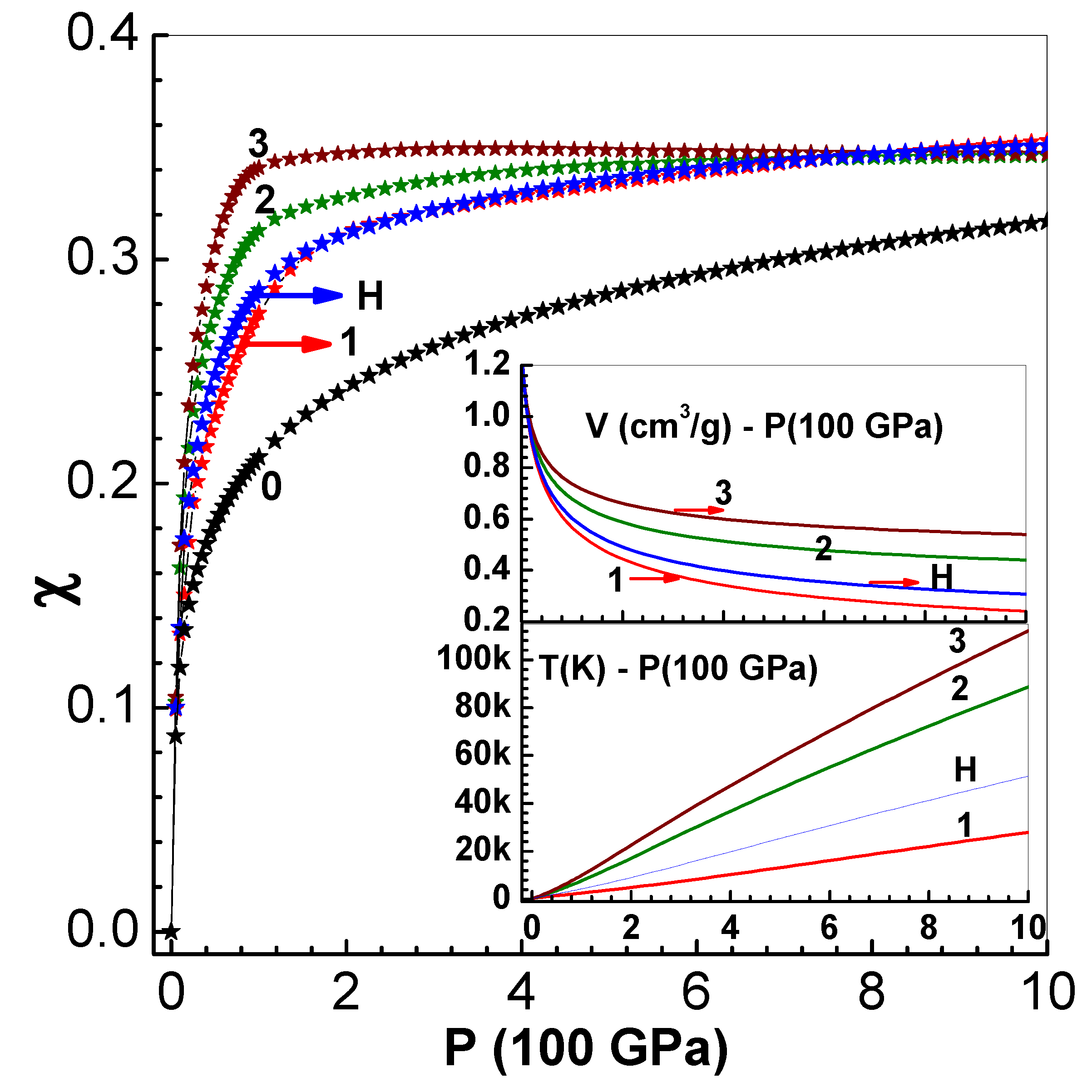
Figure 2.
Variation of V versus P along the compaction curve for Cu with initial porosity and solid density . The symbols are experimental data of Boade [35]. The inset figure shows the change in internal energy versus P as per Menikoff’s modified model (see Section 3.2).
Figure 2.
Variation of V versus P along the compaction curve for Cu with initial porosity and solid density . The symbols are experimental data of Boade [35]. The inset figure shows the change in internal energy versus P as per Menikoff’s modified model (see Section 3.2).
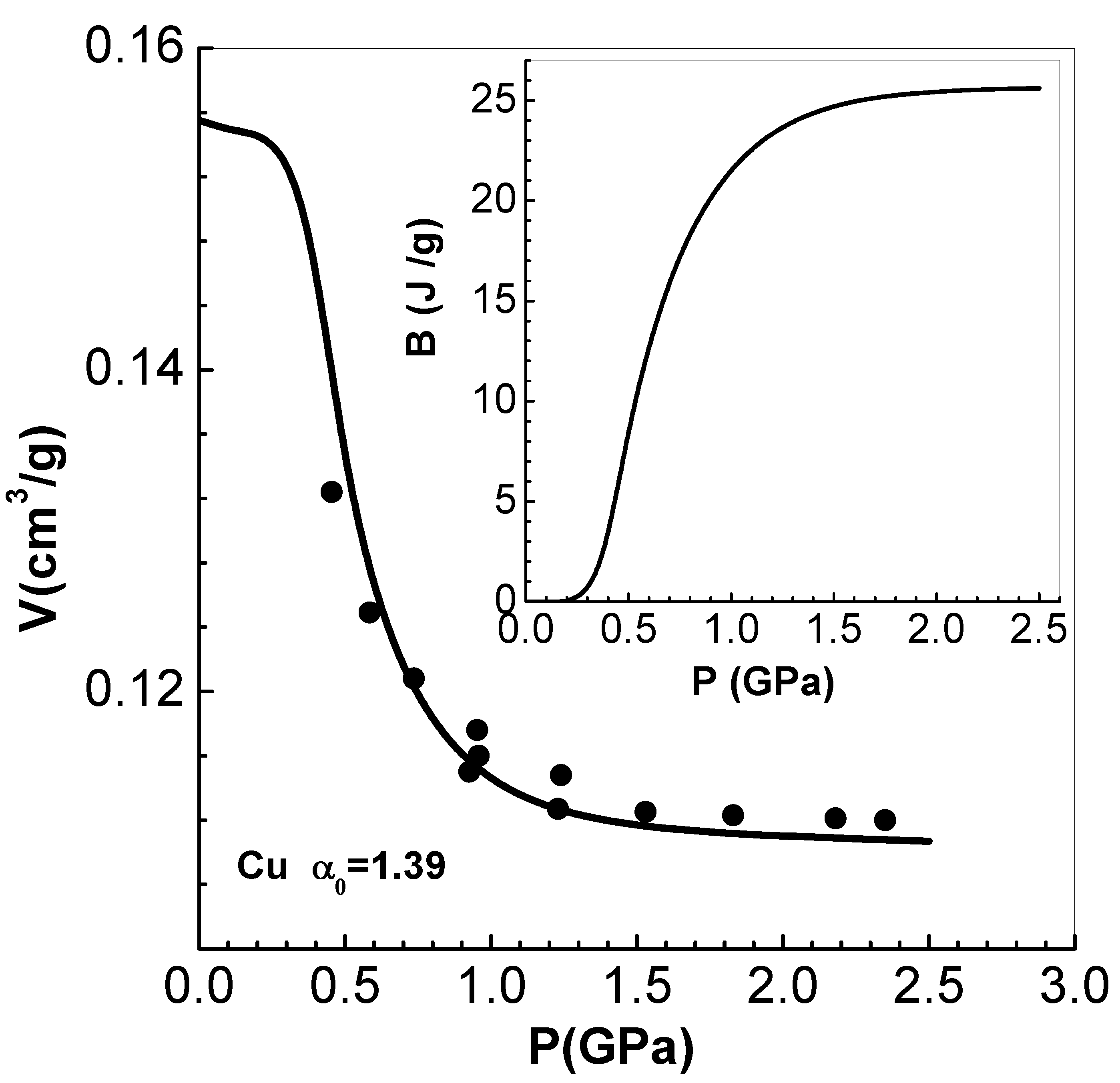
Figure 3.
Main figure compares theoretical isotherms of LiD-N (with ) at 300 K and 500 K with experimental data. Solid lines show the results of the EOS model, while the symbols are experimental data using high-pressure and high-temperature neutron diffraction [38]. The inset figure shows a comparison of Vinet’s zero-temperature isotherm with experimental data [39].
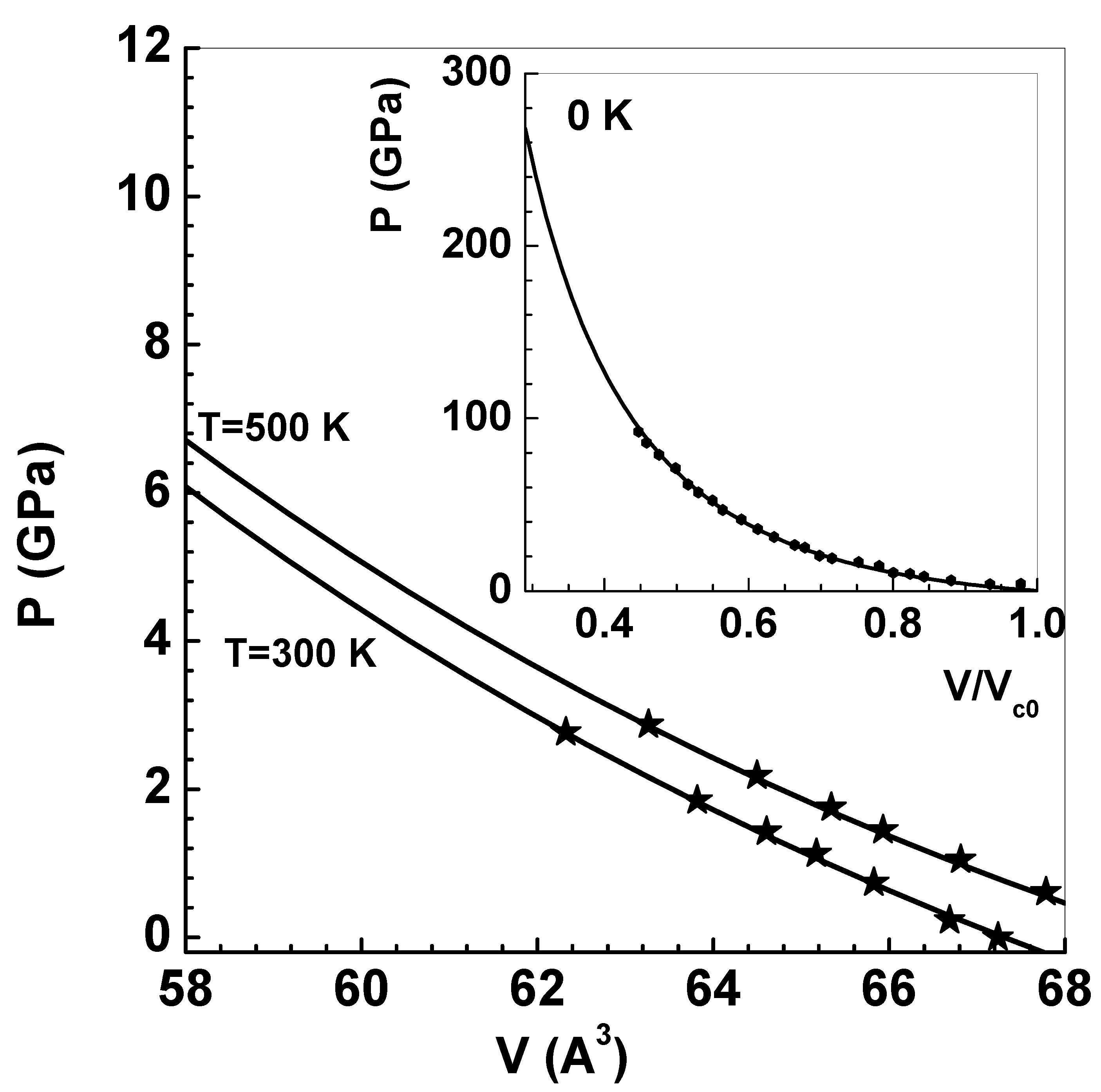
Figure 4.
Comparison of pressure P versus volume V along the principal Hugoniot with experimental data [40] (filled circles) and [41] (filled stars) up to about 1000 GPa. The inset figure shows temperature T versus pressure P and experimental data [40].
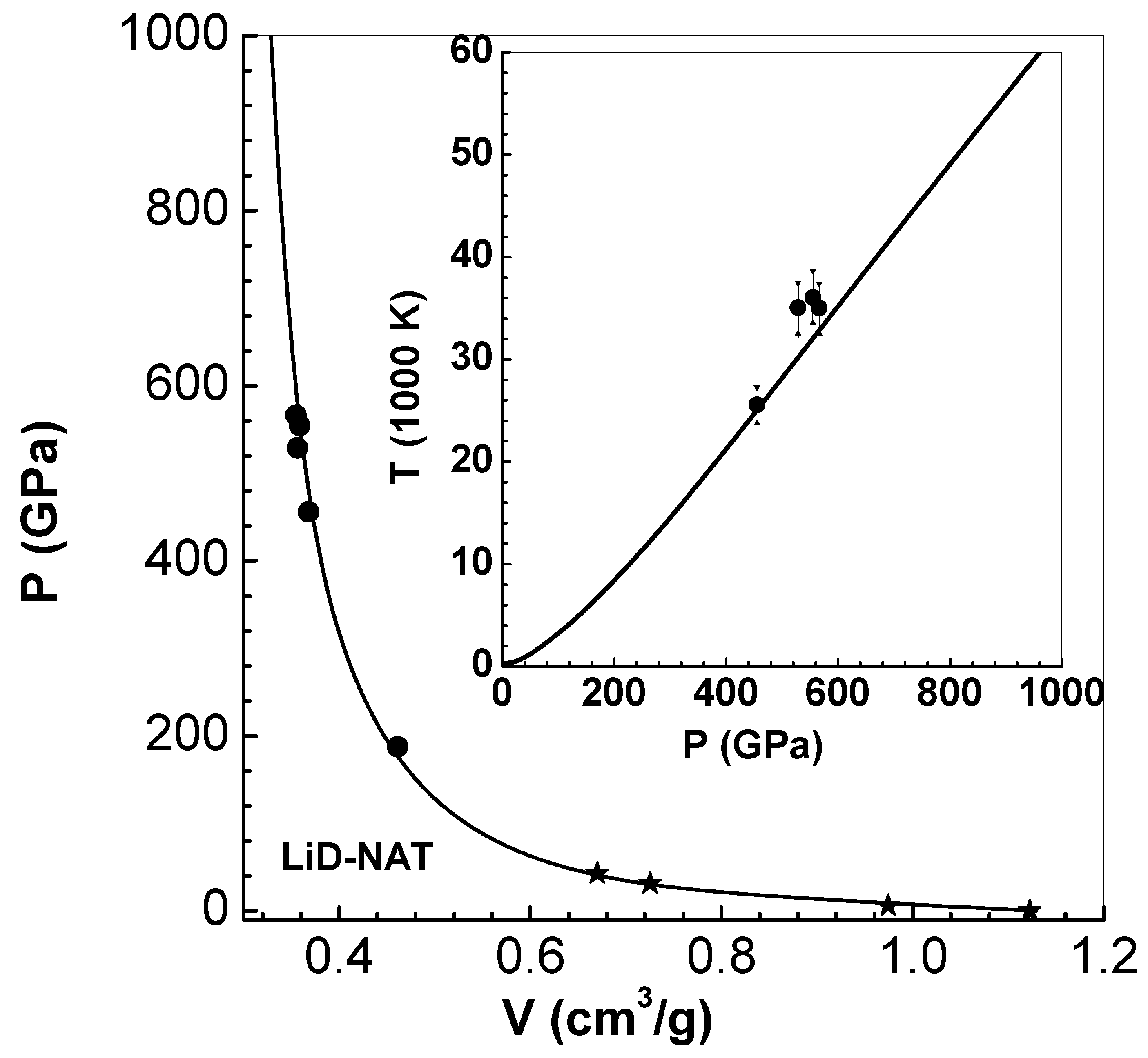
Figure 5.
Comparison of pressure P versus density along the principal and re-shock Hugoniot with experimental data [40] (filled circles) up to about 1000 GPa.
Figure 5.
Comparison of pressure P versus density along the principal and re-shock Hugoniot with experimental data [40] (filled circles) up to about 1000 GPa.
Figure 6.
Comparison of pressure P versus volume V along the principal Hugoniot, with experimental data from LASL compilation [41]. The graphs (from bottom) correspond to of solid LiD-N , solid and two porous samples. The initial porosity of the samples are shown in brackets in the legend, and successive graphs are shifted upwards by 10 units for clarity.
Figure 7.
Comparison of pressure P versus density (solid line) along the principal Hugoniot of solid ( g/cm3) with results of KSMD (filled stars for P > 100 GPa) and OFMD (filled circles) [42] (see text in Section 4.3). LASL experimental data [41] up to 45 GPa (filled stars) are also shown. The inset figure compares computed temperatures of EEOS model with those of KSMD (filled stars) and OFMD (filled circles) simulations.
Figure 8.
Comparison of pressure P versus density (solid lines) along the Hugoniot curves of solid and 4 porous ( and g/cm3) with results of OFMD (symbols) [42] (see text in Section 4.3). LASL experimental data [41] of the solid up to 45 GPa (filled stars) are also shown.
Figure 8.
Comparison of pressure P versus density (solid lines) along the Hugoniot curves of solid and 4 porous ( and g/cm3) with results of OFMD (symbols) [42] (see text in Section 4.3). LASL experimental data [41] of the solid up to 45 GPa (filled stars) are also shown.
Figure 9.
Pressure P versus fluid velocity in solid (initial density ) (curve-1), and targets with initial porosity (curve-2) and (curve-3). The symbols are LASL experimental data [41].
Figure 9.
Pressure P versus fluid velocity in solid (initial density ) (curve-1), and targets with initial porosity (curve-2) and (curve-3). The symbols are LASL experimental data [41].
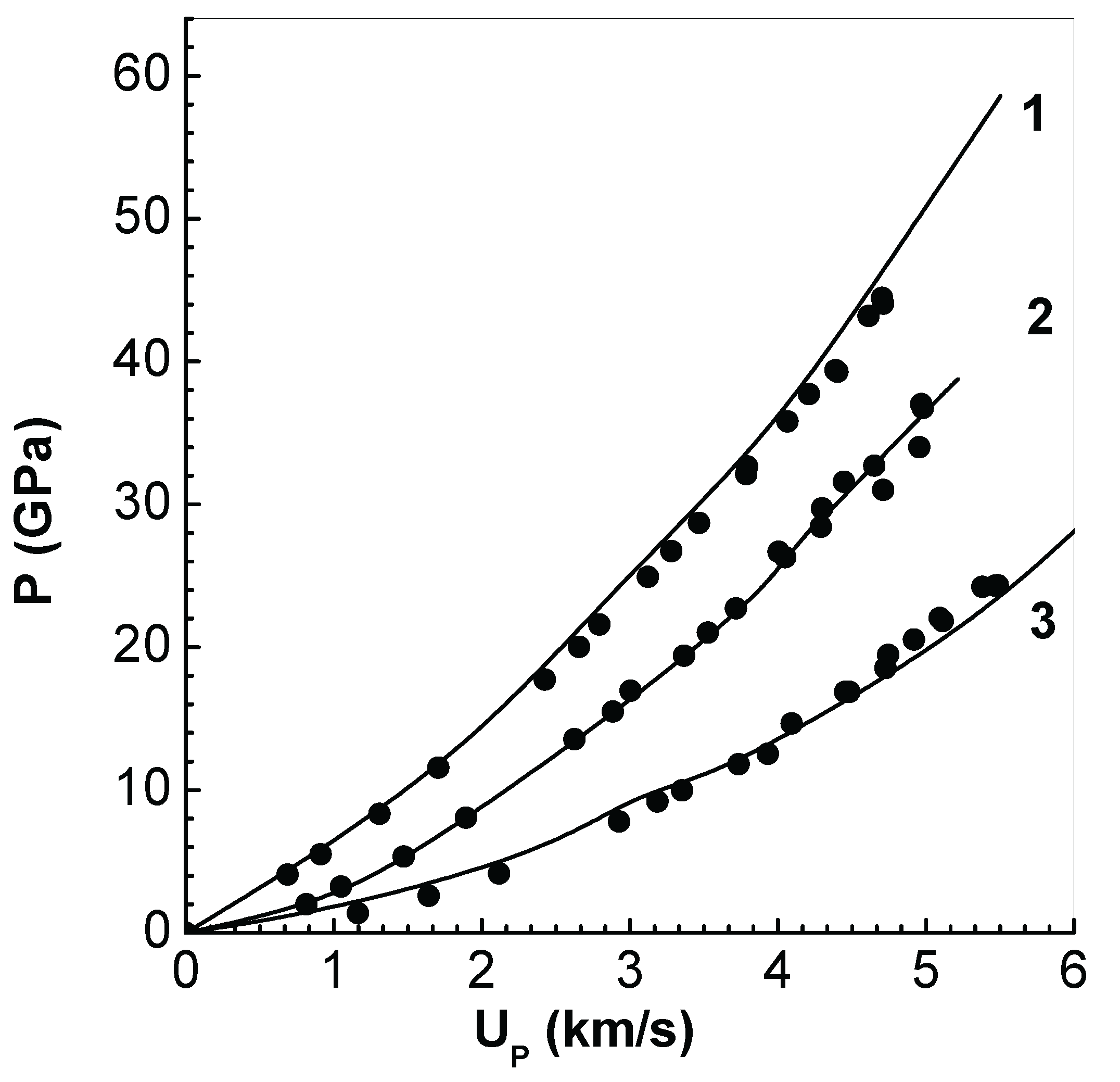
Table 1.
Fitting constants for and .
| 0 | 3.3623507 | 6.1852324 | 31.183606 | 13.860657 |
| 1 | -401.07293 | 3877.2639 | 3164.4352 | 9610.8263 |
| 2 | 2.8182514 | -0.62899210 | 7.5243122 | -1.2048560 |
| 3 | 2.9748254 | -0.71993507 | 6.9731093 | -1.1227845 |
| H | -0.42562677 | 24.168165 | 20.940494 | 62.256942 |
| 1 | 2564.6813 | -393.97924 | 701.49802 | 0.23548460 |
| 2 | 6027.1119 | 1319.3867 | 775.26105 | 0.098925459 |
| 3 | 7516.4853 | 2134.3297 | 1344.5431 | 0.13534592 |
| H | 3662.1612 | 369.97967 | 173.67388 | 0.038177599 |
; .
Disclaimer/Publisher’s Note: The statements, opinions and data contained in all publications are solely those of the individual author(s) and contributor(s) and not of MDPI and/or the editor(s). MDPI and/or the editor(s) disclaim responsibility for any injury to people or property resulting from any ideas, methods, instructions or products referred to in the content. |
© 2025 by the authors. Licensee MDPI, Basel, Switzerland. This article is an open access article distributed under the terms and conditions of the Creative Commons Attribution (CC BY) license (http://creativecommons.org/licenses/by/4.0/).
Copyright: This open access article is published under a Creative Commons CC BY 4.0 license, which permit the free download, distribution, and reuse, provided that the author and preprint are cited in any reuse.


