
Submitted:
25 July 2025
Posted:
29 July 2025
You are already at the latest version
Abstract
To demonstrate the difference between non-ideal experiments and idealized analytical models, bending vibrations of a frame structure have been analyzed in the context of hands on teaching in structural dynamics. Both experimental modal analysis and model based evaluation of system dynamics have been performed. The investigations have been limited to mechanical vibrations in the low frequency range. It has been found that even simple mechanical models are very useful to explain, to understand, and to validate experimental results. The latter have been derived from one key principles of analytical dynamics – the LAGRANGE formalism. The article is written for students in mechanical engineering and related fields as well as for the academic community. The latter could use the results as a benchmark problem in academic teaching as well as in applied research.
Keywords:
structural dynamics
; experimental modal analysis
; analytical dynamics
1. Introduction
Structural dynamics is an important topic in the theory of mechanical vibrations [1,2]. It is a traditional but still relevant field in many engineering studies. It especially important for mechanical and civil engineering as well as for automotive, aeronautical and aerospace engineering [3,4]. Beside these classical disciplines structural dynamics is closely connected to engineering acoustics [5], analytical and numerical methods of applied mathematics [6] as well as to the theory of signals and systems [7] including experimental methods [8,9,10,11]. Thus, structural dynamics is a cross-disciplinary approach (as also shown in the present paper) and it is therefore impossible to honor the important contributions of all scientists working in this field. For this reason, the list of text book references presented in the present paper is limited to a very small number that nonetheless allows for finding a starting based on well-established text books.
Furthermore, structural dynamics is an academic field with ongoing actual development. This is true for theoretical research as well as for the development and application of experimental methods (such as experimental modal analysis) in several disciplines of engineering. A general overview on advances in vibration engineering and structural dynamics covering a broad range of topics such as rotor dynamics, structural vibrations of beam and shell structures, and structural vibrations in civil engineering is given in [12]. A particular problem in structural dynamics is given by the presence of non-linear effects. The latter have to be taken into account in numerical simulations [13,14] as well as in experimental investigations [15,16].
Another novel trend in structural dynamics is the application of wavelet transform methods [17] in modal analysis and damage detection approaches. Identification of modal parameters using the wavelet transform has been discussed in [18]. A case study in which the continuous wavelet transform (CWT) has been applied to perform structural dynamic analysis of a beam structure has been presented in [19]. Experimental modal analysis based on CWT applied to the transient response of a beam structure is discussed in [20], whereas the damage detection based on a wavelet method has been presented in [21].
Recent studies in which experimental modal analysis has been applied to aircraft structures have been published in [22-26]. Model analysis applied to vehicle structures have been discuses in [27-30]. Naturally, modal analysis plays also an important role for the analysis of classical structures in civil engineering such as buildings and bridges, compare [30,31]. However, also timber structure have been analyzed and characterized by the application of modal analysis [32,33]. Furthermore, experimental modal analysis is nowadays also an established approach in polymer science [34].
Considering all these references it can be concluded that structural dynamics including some highly specialized analysis methods such as experimental modal analysis or wavelet transform methods is still an evolving a research area that is relevant for many disciplines of engineering. Thus, it is still also a relevant topic in the development of academic curricula [35].
If so many references can be found, one question arises. This question can be formulated in the following way: Is it necessary to publish a paper on a particular problem? To answer this question it can be useful to remember a typical challenge in teaching structural dynamics. The latter is connected with the establishment of proper non-trivial models. On the one hand these models must be capable to describe the vibrational behavior of the analyzed system. On the other hand these models must not be sophisticated in order to find solutions without high-end simulation techniques. However, the mechanical models that can be found in many textbooks on structural dynamics are highly idealized. Therefore, it is possible to derive analytical solutions for many sample problems.
But, it is not easy to design simple experiments that are useful to demonstrate the results derived from some of these basic models. This is especially true in the context of hands on teaching in structural dynamics including class-room experiments based on structures with non-ideal properties such as incomplete realization of symmetry conditions or imperfections in the realization of boundary conditions. Furthermore, the application of sensors as well as the connection of actuators can cause effects that are not included in a basic mechanical model of a structure. Unfortunately, the effects caused by these imperfections will be found in the experimental data. The task for the engineer is however, to interpret the measurement data based on simple but at the same time also adequate and reliable models.
The present paper is an attempt to contribute to this teaching challenge. It is written for the academic community as well as for master students in engineering science. Even if it is not a classical research article, the problem described in the present paper in great detail can contribute to applied research, if it is used as a benchmark model. The latter is designed to demonstrate the difference between non-ideal experiments and idealized analytical models used to describe bending vibrations of a frame structure.
The paper is structured as follows. Experimental investigations in time-domain and in frequency-domain including experimental modal analysis are described in section 2. Analytical models (applied to understand the experimental findings) are discussed in section 3. The paper closes with section 4 presenting a short summary of the main findings.
2. Experimental Investigations
2.1. Description of Frame Structure
The frame structure analyzed in a particular class-room setting is shown in figure 1. It consists of two vertical parts of length and one horizontal part of length . It is clamped at both ends. The structure has a rectangular cross section with width and height . It is made of aluminum. As also shown in figure 1 three concentrated weights are connected at the positions . The specific data are given in table 1.
As also shown in figure 1, three ordinary acceleration sensors (labeled with “Left”, “Middle”, and “Right”, each having a weight of approximately 0.01 kg) are connected to the horizontal part of the frame structure. The structure is driven by an electro-dynamical exciter. The connection between structure and actuator is established by a soft rubber band. The excitation signal is generated by the soundcard of an ordinary personal computer using a sampling rate of 44.1 kHz. All cables have been arranged in such a way that any friction between structure and cable has been avoided.
2.2. Time-Domain and Frequency-Domain Analysis
At first the system response to a step-input signal (manually applied by hand) has been analyzed. Only the system outputs have been determined. The results are shown in figure 2. The time-domain response is shown left considering the acceleration signals normalized to the peak value for each channel. The associated magnitudes of the Fourier spectra are shown right. The latter are also normalized to the maximum value.
It can be seen that the frame structure is slightly damped and the system response is based on four natural modes. It can clearly be seen that the first natural mode dominates the response measured at the center position (“Middle”) of the frame structure. Furthermore, it can be seen that the acceleration sensor at the center position is located close to nodal points of the second and the third mode.
To analyze transfer behavior of the structure the experiment has been repeated using a sine-sweep as input signal. Thus, the response (acceleration) is measured at three positions due the single system input (voltage) applied to the electro-dynamical exciter. The time-domain behavior and the frequency-domain behavior of the input signal is shown in figure 3. Because the highest natural frequency is below 25 Hz, the frequency range for the excitation signal is between 0 Hz and 25 Hz. It can be seen that the magnitude of the excitation signal is constant over the main part of the analyzed frequency range.
The time-domain representation and the frequency-domain representation of the three output signals are shown in figure 4. The system output peaks at the resonance frequencies. Because the system is only slightly damped it can be expected that natural frequencies and resonance frequencies are nearly identical.
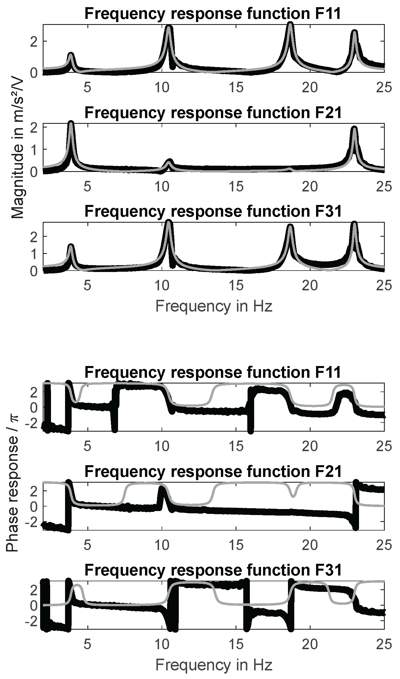
In order to identify both natural frequencies and the associated mode shapes the frequency response functions (FRF) have been determined. Magnitude response and phase response curves are shown in figure 5. The associated real part of the FRF’s as well as the imaginary part of the FRF’s are shown in figure 6. The resonance frequencies and the associated modes (identified on the basis of these FRF’s) are listed in Table 2 und Table 3. All modes are normalized to the response measured at the “Left” sensor position.
It can be seen that the second and third mode are not identical in frequency but identical in shape. This is an interesting result. In both modes the signals measured at the “Left” and the “Right” sensor position are opposite in phase and more or less identical in magnitude. The “Middle” sensor position is a nodal point for both mode shapes.
To confirm this result the modal assurance criteria proposed in [36] has been applied. This criteria is valid for both real valued and complex eigenvectors. It is calculated according to equation (1)
where, is the i-th eigenvector and is the j-th eigenvector. The value is in the range . The minimum value indicates that the modes i and j are completely independent to each other. The maximum value indicates that the mode shape of the i-th mode is completely identical to the mode shape of the and j-th mode.
All calculated modal assurance values are listed in table 4. The results presented in this table proof that the eigenvectors and represent identical mode shapes. However, these mode shapes are orthogonal to the eigenvectors represented by and . Furthermore, the eigenvector is orthogonal to the eigenvector .
2.3. Synthesis of Mode Shapes
To complete the experimental investigations models for the FRF’s have been analyzed by experimental model analysis. Because the resonance frequencies are clearly separated the simple method of peak-pinking (PP) [10] has been applied. This method is based on the i FRF’s of each modal degree of freedom (DOF) – also known as generalized coordinates. These FRF’s can be represented by rational functions such as
where is the i-th generalized mass, is the modal damping in the i-th mode, is the angular frequency associated to the i-th natural frequency , and is the angular frequency associated with the frequency of excitation . The modal damping parameter have been determined by the half-bandwidth-method [10] for each resonance frequency such as
where is the frequency at the -3dB point left to the i-th resonance frequency, and is the frequency at the -3dB point right to the i-th resonance frequency. All modal damping parameter are listed in table 5. The data indicate that the system is indeed slightly damped. The maximum modal damping is below 3%.
To perform experimental modal analysis using PP it is also necessary to determine the peak value of the magnitude response, compare figure 5, for each resonance frequency.
These data are summarized in table 6. They are required to calculate the modal contribution of the i-th mode to the system response at position r according to the excitation acting at position s such as
The connection between the real world FRF’s and the FRF’s of the modal coordinates is established by the modal transformation such as
where the modal matrix
contains the eigenvector of each mode such as
It is a strait forward calculation to proof that the three real world FRF’s of the analyzed system can be represented by the following transfer function models (TFM’s)
A comparison between the measured FRF’s and the identified TFM’s is shown in figure 5. The match in magnitude is nearly perfect and the similarity in phase is sufficient considering the application of the simple PP method.
Figure 5.
Identified transfer function models (in gray) compared to measured FRF’s.
However, even if adequate response models can be identified by a very simple approach, it is still necessary to explain the similarities between the mode shape of the second resonance on the one hand and the mode shape of the third resonance on the other hand. To explain this result analytical analysis of simple models can be helpful.
3. Theoretical Analysis – Understanding the Experimental Data
The interpretation of experimental data is much more intuitive, if the results can be mapped to the behavior of models of vibrating structures. These models should be as exact as necessary and as simple as possible at the same time. It is obvious that the frame structure shown in figure 1 executes bending vibrations in vertical direction. As shown in [2] the associated vibration modes can be described by a combination of global shape functions and generalized coordinates such as
In our investigation we will consider only the first three bending modes assuming simply supported boundary conditions. For this reason the set of shape functions reads
Because the kinetic energy and the potential energy of the physical structure vibrating in the i-th mode is equivalent to the kinetic energy and potential energy of the i-th generalized structure, compare [2], we can calculate the elements of the mass matrix such as
where is the DIRAC distribution and is the n-th concentrated mass at the position . The elements of the stiffness matrix depend on the curvature as known from BERNOULLI’s beam theory. These elements are given by the following integral
Considering a constant density as well as a constant cross section the mass matrix is given by the superposition of the contributions of the continuous beam structure, compare first summand in equation (13),
and the contributions of the concentrated point mases. The latter are given by symmetric matrices that in general contain non-zero off-diagonal elements. These contributions are defined by equation (14)
where
is a dimensionless length, indicating the position of the n-th concentrated mass on the horizontal part of the frame structure, compare figure 1 and table 1. Considering a constant bending stiffness the solution of equation (12) reads
In order to derive the equation of motion we have to formulate the expressions for both the kinetic energy T and the potential energy U based on the generalized coordinates such as
Applying LAGRANGE’s principle
the equations of motion are given by
To determine the natural frequencies for the bending modes it is necessary to find the zeros of the associated characteristic polynomial. This problem reads
However, the solution of equation (2) only yields three natural frequencies associated with three bending modes. A simple model that can be used to explain the fourth resonance frequency determined in the experimental investigation is still needed. Such a model can be derived, if the bending vibration of the vertical parts of the frame structure is taken into account. If the horizontal part of the frame structure (including the three concentrated mass points) is seen as a concentrated rigid mass connected to two springs acting in parallel (horizontal parts of the frame structure) we can establish a fourth DOF. The mass associated with this horizontal DOF is given by
whereas the associated effective stiffness reads
The multiplier “2” represents the fact that the two vertical parts of the frame structure are acting in parallel. The second term in equation (22) represents the bending stiffness of a beam that is fixed at one and free at the other end, compare [2]. The formula for the associated natural frequency is given in equation (23).
Numerical data for the four natural frequencies and based on the parameter given in table 1 are listed in table 7. It can be seen that the three natural frequencies calculated for bending vibrations in vertical direction are in fair agreement with the resonance frequencies determined for the 1st, 2nd, and 4th mode shape in the experimental investigations.
The natural frequency calculated from the simple model describing the horizontal vibration is in fair agreement with the 3rd resonance frequency determined in the experimental investigations. It can be concluded that due to imperfections in the experimental setup this horizontal mode couples with the 2nd vertical bending mode that is in its shape similar to 3rd mode shape determined for a resonance frequency of 18.7 Hz.
4. Conclusions
The intension of this paper was to present an intuitive but not trivial problem of structural dynamics. This problem has been demonstrated to students of aeronautical engineering, automotive engineering and mechatronics in many courses over the last decade. The demonstration by itself is simple. However, because of imperfections – going hand in hand with hands on teaching – it is not easy to interpret the results. In order to overcome this problem it is helpful to apply adequate dynamical models that can be derived from the principles used in structural dynamics. The main conclusion can be summarized as follows:
- The established methods of experimental modal analysis are useful to demonstrate the determination of modal parameters such as resonance frequencies, mode shapes and modal damping for non-trivial test structures.
- The interpretation of experimental results is easier, if models capable to describe the dynamical behavior of the structure are taken into account. These models should not be sophisticated in order to derive robust analytical solutions in a short period of time.
As written in the introduction this paper has been written for both the scientific community and students of engineering science. The analyzed problem has been described in great detail. It is very easy to reproduce. Thus, it could serve as a benchmark model to validate new experimental techniques. However, it is also possible to use the results for the validation of new numerical approaches.
The paper contains all relevant data and equations. All findings can be reproduced without knowledge of the few but very excellent references. This can be advantageous for students of advanced coursed in structural dynamics and related field, because a non-trivial problem is described by experimental and analytical methods in a compact and contestant way. Furthermore, everyone teaching structural dynamics can easily derive a simple demonstration experiment based on the published data. Perhaps it is for this reason a small contribution to stimulate a deeper interest in structural dynamics.
Finally it is necessary to comment on the following question: How the presented setup and analysis may be used for benchmarking experimental techniques or validating numerical approaches? One answer to this question can be given considering non-standard analysis methods such as wavelet transform methods, compare [17-21]. These methods are not necessary to analyze the problem presented in the present paper. However, if new methods in structural health monitoring [11] and damage detection [21] based on experimental structural analysis have to be validated, the presented experiment could be used as a starting point for the undamaged structure. Because it is simple to manufacture copies of the presented structure it is also easy to produce twins including defined artificial damage (represented by slots and gaps of different size and shape). Thus, the original structure in combination with artificially damaged twins can serve as benchmark models to validate damage detection approaches.
Another benchmark-possibility is given by the fact that the point masses shown in figure 1 are connected by screws. In imperfect connection (this could also be interpreted as a particular aspect of damage) would result in additional damping caused by dry-friction. Thus, the experiment presented in this paper could also be used to validate non-linear models in structural dynamics that include damping models based on dry friction between a base structure (beam) and attached substructures (concentrated point masses).
A last benchmark-idea can be motivated considering the fact that a detailed modal analysis of large structures results in a large data set that has to be analyzed. At this point artificial intelligence and machine learning methods become relevant. Machine learning in the context of non-linear structural dynamics has been discussed in [37]. However, a simplified analytical model has been used to generate the data. The presented experiments could be a simple alternative to generate a sufficient set of real world data. This is especially true, if random excitation signals are used. A machine-learning based approach to structural health monitoring and its application to a realistic bridge structure has been presented in [38]. The structure analyzed in this reference is more sophisticated compared to the structure presented in this paper. However, the methodology applied in [38] could be verified using the well-defined simple structure presented in this article. The same holds for the approach presented in [39].
The state of the art in automated operational modal identification has been summarized in [40], considering various AI-driven approaches. The authors conclude that: “Challenges such as identifying double and multiple modes, modes with low observability, damped modes and systems with high damping, and systems subjected to combined excitations (random and harmonic) can be considered key challenges faced by intelligent system identification algorithms.” The system presented in this article generates a double mode (as shown for the 2nd and 3rd mode shape), if the excitation is not harmonic. Furthermore, it is easy to choose nodal points at which a mode shape is difficult to observe (this is especially true for center position of the bean at the 2nd and 3rd natural frequency). Finally, the presented problem is well suited to combine harmonic and random excitation signals. Thus, it is possible for the reader to define research questions inspired by [40] that could be investigated on the basis of the presented well-defined benchmark model.
References
- Seto, W. W. Mechanical Vibrations, 1st ed.; McGRAW-HILL, New York, USA, 1964.
- Brommundt, E.; Sachau, D. Schwingungslehre mit Maschinendynamik, 1st ed.; Springer Berlin, Heildelberg, Germany, 2008.
- Gasch, R.; Knothe, K. Strukturdynamik – Band1: DiskreteSysteme, 1st ed.; Springer, Berlin, Germany, 1987.
- Gasch, R.; Knothe, K. Strukturdynamik – Band2: Kontinua und ihre Diskretisierung, 1st ed.; Berlin, Germany, 1989.
- Fahy, F.; Gardonio, P. Sound and structural vibration, 1st ed.; Academic Press, UK, 2007.
- Börm, S.; Mehl, C. Numerical methods for eigenvalue problems, 1st ed.; De Gruyter, Berlin, Germany, 2012.
- Oppenheim, A. V.; Willsky, A. S.; Nawab, S. H. Signals and Systems, 2nd.; Prentice Hall, New Jersey, USA, 1997.
- Randall, R. R. Application of B&K equipment to frequency analysis, 2st ed.; Nærum, DK, 1977.
- Broch, J. T. Mechanical vibration and shock measurements, 2st ed.; Larsen and Søn, Søborg, DK, 1980.
- Ewins, D. J. Modal testing. Theory, practice and application, 2nd ed.; WILEY, Hoboken, USA, 2000.
- Randall, R. R. Vibration based condition monitoring, 1st ed.; WILEY, Hoboken, USA, 2021.
- Beltrán-Carbajal, F. Advances in vibration engineering and structural dynamics, 1st ed.; INTECH, Rijeka, Croatia, 2019.
- Lee, Y.-y. Free Vibration Analysis of Nonlinear Structural-Acoustic System with Non-Rigid Boundaries Using the Elliptic Integral Approach. Mathematics 2020, 8(12), 2150. [CrossRef]
- Maio, D. D. A novel analysis method for calculating nonlinear frequency response functions. Journal of Structural Dynamics 2025, 3, pp. 30-57, DOI: 10.25518/2684-6500.242.
- Xu, Z.; Pei-yao, X.; Hui, L.; Chen, C.; Peng-yao, S.; Da-wei, G.; Da-shuai, S.; He, L.; Qing-kai, H.; Wen, B. The analysis of nonlinear vibration characteristics of fiber-reinforced composite thin wall truncated conical shell: Theoretical and experimental investigation. European Journal of Mechanics - A/Solids 2024, 105, 105268. [CrossRef]
- Dolbachian, L.; Harizi, W.; Aboura, Z. Experimental linear and nonlinear vibration methods for the structural health monitoring (SHM) of polymer-matrix composites (PMCs): A literature review. Vibration 2024, 7, pp. 281-325. [CrossRef]
- Chui, C. An introduction to wavelets, 1st ed.; Academic Press, New York, USA, 1992.
- Lardies, J.; Gouttebroze, S. Identification of modal parameters using the wavelet transform. International Journal of Mechanical Sciences 2002, 44(11), pp. 2263-2283. [CrossRef]
- Oviedo, T. C. A.; Mendez, Q. J. E. Structural dynamic analysis using wavelets. Journal of Physics: Conference Series 2019, 1160 012016. [CrossRef]
- Régal, X.; Cumunel, G.; Bornert, M.; Quiertant, M. Assessment of 2D digital image correlation for experimental modal analysis of transient response of beams using a continuous wavelet transform method. Applied Sciences. 2023, 13, 4792. [CrossRef]
- Dziedziech, K.; Staszewski, W.J.; Mendrok, K.; Basu, B. Wavelet-based transmissibility for structural damage detection. Materials 2022, 15, 2722. [CrossRef]
- Gasparetto, V. E. L.; Machado, M. R.; Carneiro, S. H. S. Experimental modal analysis of an aircraft wing prototype for SAE Aerodesign Competition. Dyna 2020, 87(214), pp. 100-110.
- Molina-Viedma, Á.; López-Alba, E.; Felipe-Sesé, L.; Díaz, F. Full-field operational modal analysis of an aircraft composite panel from the dynamic response in multi-impact test. Sensors 2021, 21, 1602. [CrossRef]
- Radha Krishna, K. R.; Jadhav, S. D.; Mishra, A. K. Comparative modal analysis on different aircraft wing models. International Journal of Enhanced Research in Science, Technology & Engineering 2023, 12(12), pp. 42-49, ISSN: 2319-7463.
- Volkmar, R.; Soal, K.; Govers, Y.; Böswald, M. Experimental and operational modal analysis: Automated system identification for safety-critical applications. Mechanical Systems and Signal Processing 2023, 183, 109658. [CrossRef]
- Scinocca, F.; Nabarrete, A.; Santos, F. L. Uncertainty quantification in the modal analysis of aircraft stiffeners: A perturbation technique approach in SFEM. Engineering Structures 2025, 323, 119187. [CrossRef]
- Chen, H.; Lu, C.; Liu, Z.; Shen, C.; Sun, Y.; Sun,M. Structural Modal Analysis and Optimization of SUV Door Based on Response Surface Method. Shock and Vibration 2020. [CrossRef]
- Longoni, F.; Hägglund, A.; Ripamonti, F.; Pennacchi, P.L.M. Powertrain modal analysis for defining the requirements for a vehicle drivability study. Machines 2022, 10, 1120. [CrossRef]
- Peng, F.; Chen, L.; Ye, J.; Yan, F. A method for identifying common and unique issues in body in white dynamic stiffness based on modal contribution analysis. Sci Rep 2025, 15, 11911. [CrossRef]
- Li, J.; Bao, T.; Ventura, C. E. A robust methodology for output-only modal identification of civil engineering structures. Engineering Structures 2022, 270, 114764. [CrossRef]
- Golnary, F.; Kalhori, H.; Liu,W.; Li, B. Vehicle-based autonomous modal analysis for enhanced bridge health monitoring. International Journal of Mechanical Sciences 2025, 287, 109910. [CrossRef]
- Bondsman, B.; Peplow, A. Experimental modal analysis and variability assessment in cross-laminated timber. Mechanical Systems and Signal Processing 2025, 228, 112466. [CrossRef]
- Marciniak, P.; Pawlak, Z.M.; Wyczałek, I. The use of experimental modal analysis in modeling the complex timber structure of a historical building. Appl. Sci. 2024, 14, 8517. [CrossRef]
- Nguyen, H.T.; Crittenden, K.; Weiss, L.; Bardaweel, H. Experimental modal analysis and characterization of additively manufactured polymers. Polymers 2022, 14, 2071. [CrossRef]
- Yang, H.; Sun, J. Reform and practice of teaching “Structural Dynamics and Its Engineering Applications” Based on the OBE concept. Global Journal of Engineering Sciences 2024, pp. 1-4, ISSN: 2641-2039, DOI: 10.33552/GJES.2024.11.000772.
- Vacher, P.; Jacquier, B.; Bucharles, A. Extensions of the MAC criterion to complex modes, Proceedings of ISMA2010-USD2010 Conference, Leuven, Belgium, 2010, pp. 2713-2726, https://past.isma-isaac.be/isma2010/.
- Worden, K.; Green, P. L. A machine learning approach to nonlinear modal analysis. Mechanical Systems and Signal Processing 2015, 84(B), pp. 34-53. [CrossRef]
- Civera, M.; Mugnaini, V.; Fragonara, L. Z. Machine learning-based automatic operational modal analysis: A structural health monitoring application to masonry arch bridges. Structural Control and Health Monitoring 2022, 3, pp. 1-23. [CrossRef]
- Mugnaini, V.; Fragonara, L. Z.; Civera, M. A machine learning approach for automatic operational modal analysis. Mechanical Systems and Signal Processing 2022, 170, 108813. [CrossRef]
- Mostafaei, H.; Ghamami, M. State of the art in automated operational modal identification: Algorithms, Applications, and Future Perspectives. Machines 2025, 13, 39. [CrossRef]
Figure 1.
Setup for experimental investigations.
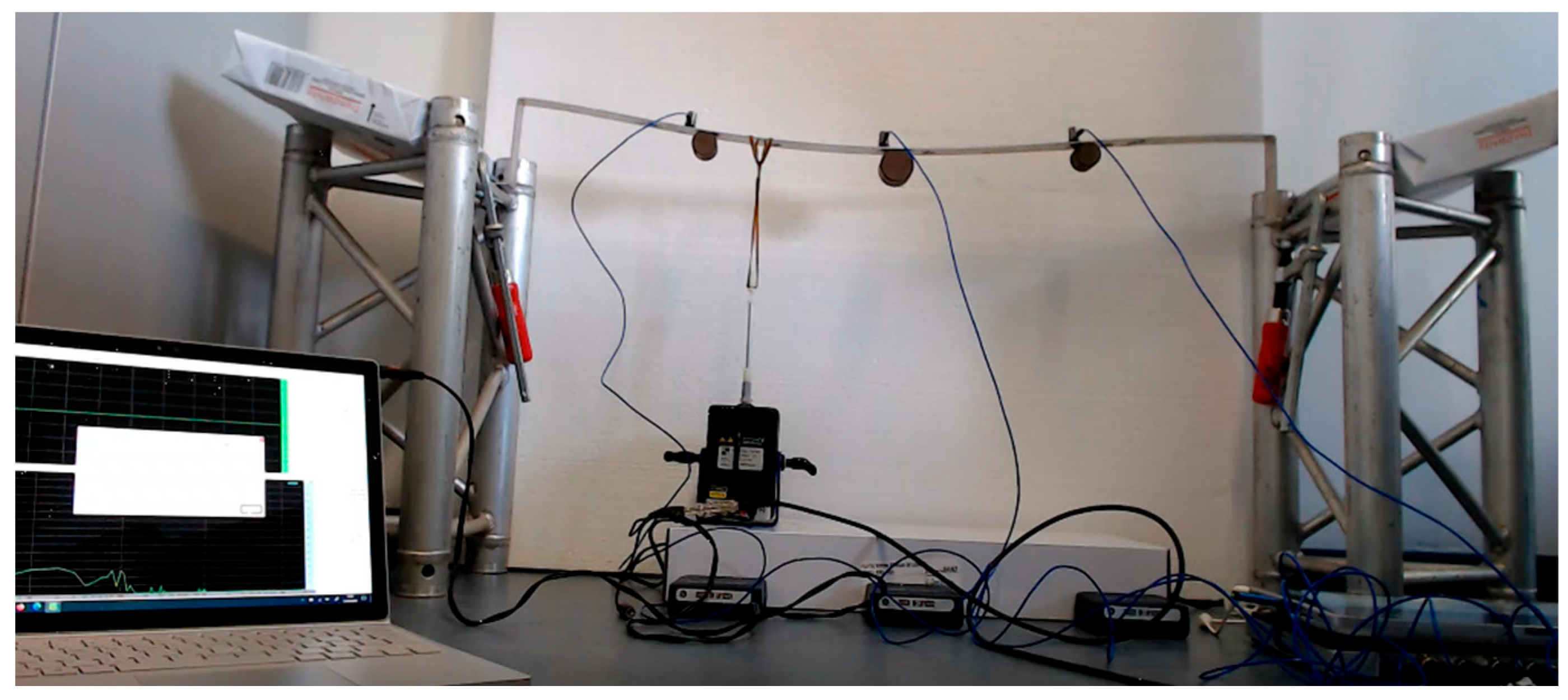
Figure 2.
Time response and frequency response of system to step-signal input.
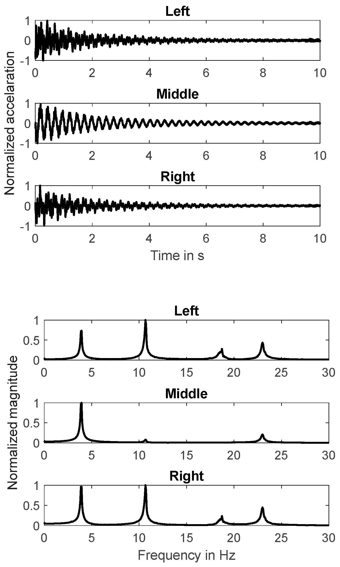
Figure 3.
Time series and power spectrum of sweep-signal input.
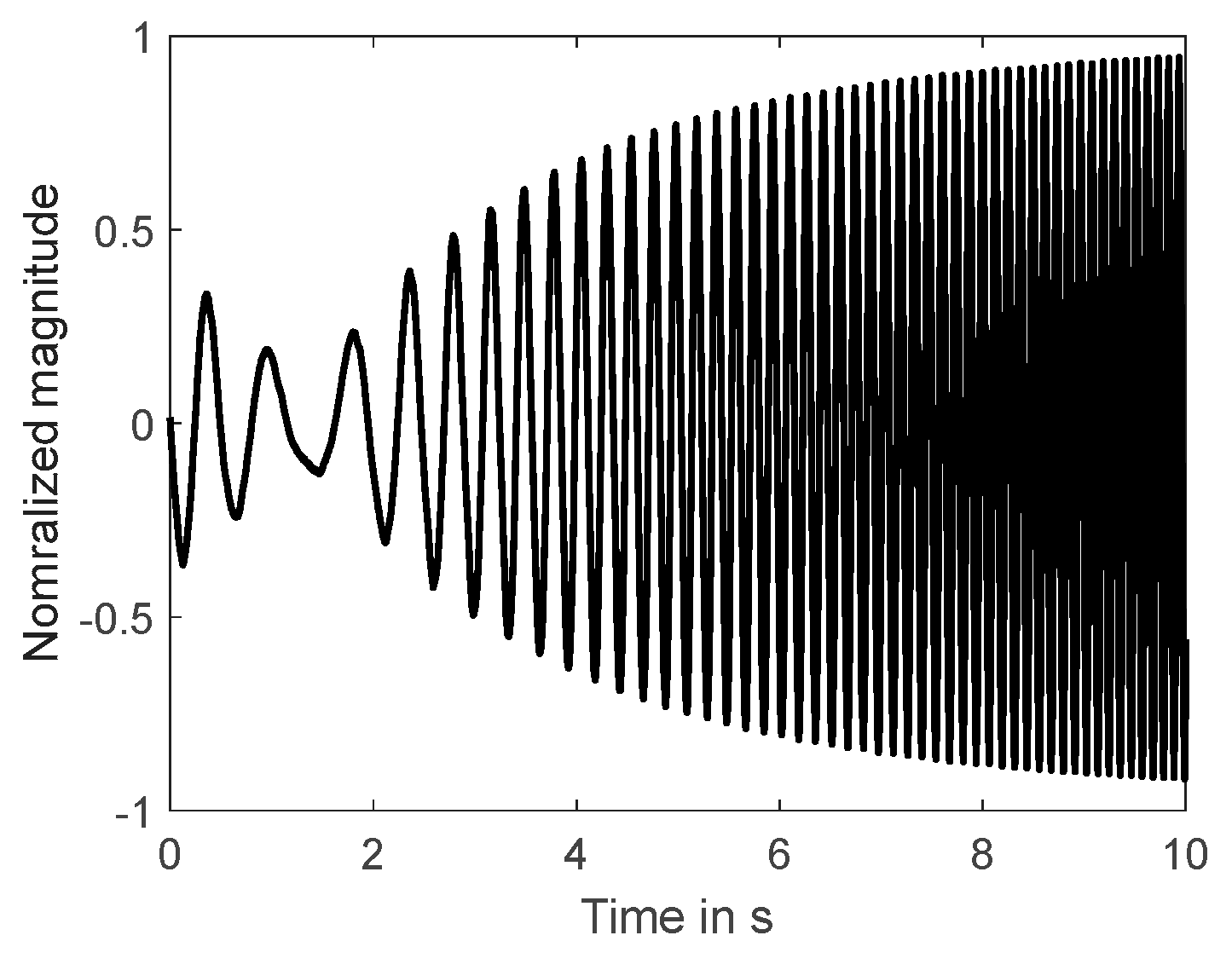
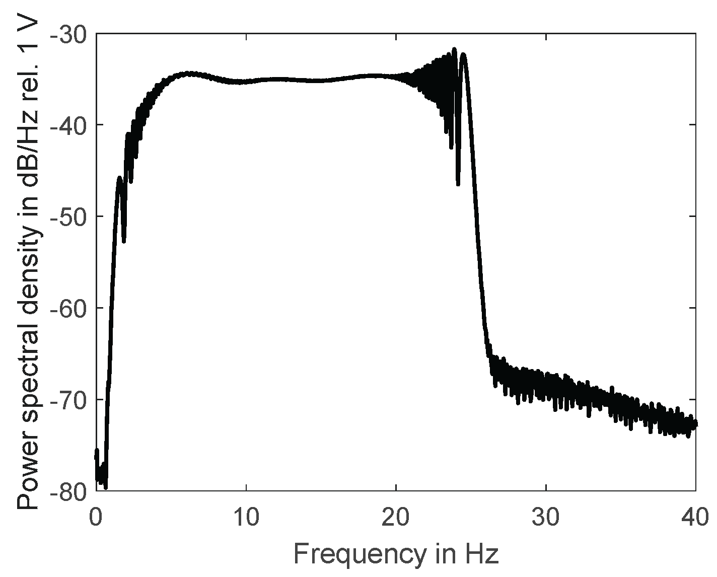
Figure 4.
Time response and frequency response of system to sweep-signal input.
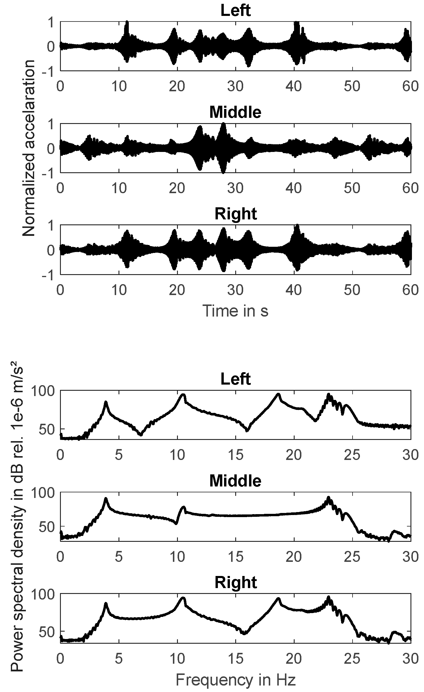
Figure 5.
Frequency response curves (F11 -> Left, F21 -> Middle, and F31 -> Right).
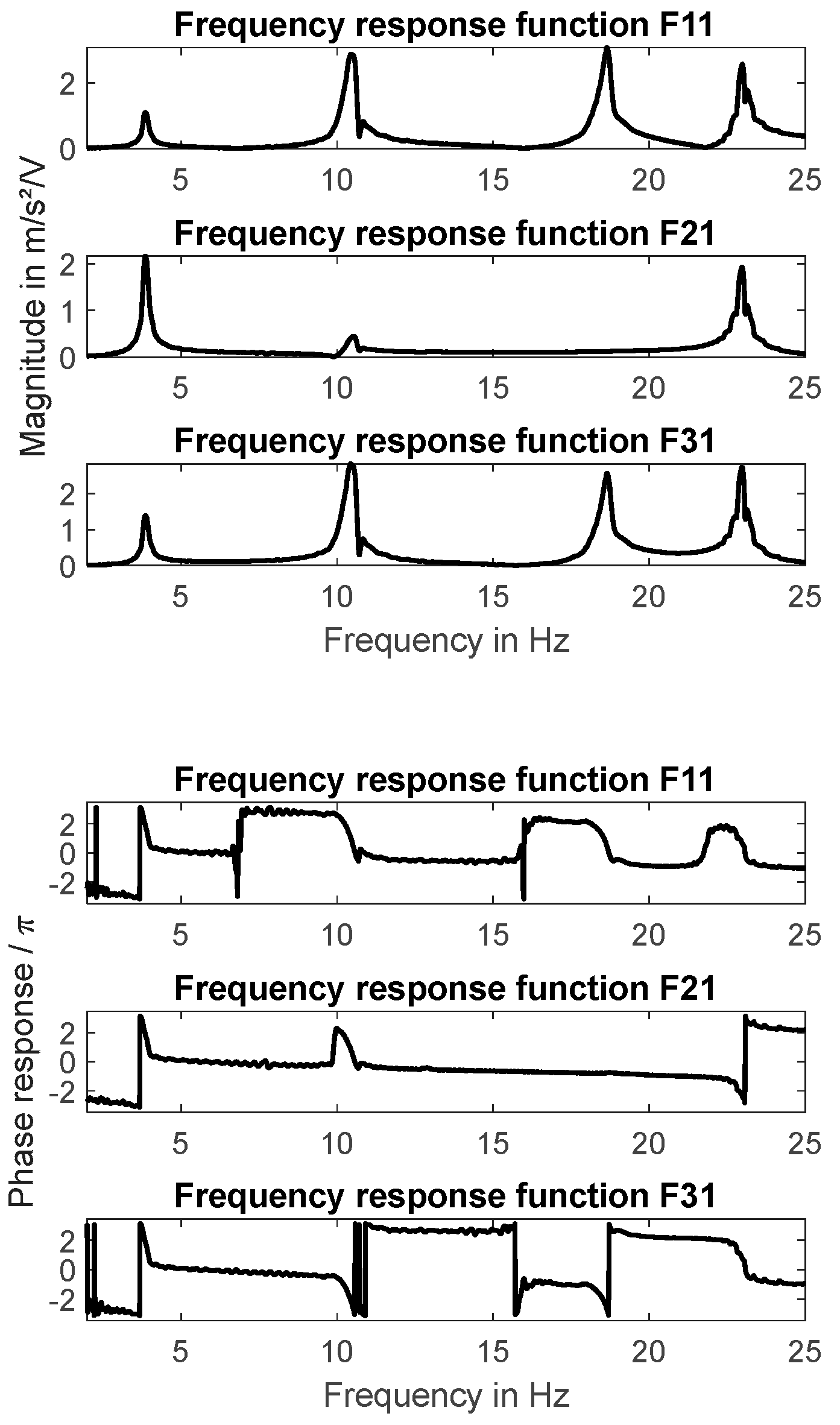
Figure 6.
Real part and imaginary part of FRF’s (F11 -> Left, F21 -> Middle, F31 -> Right).
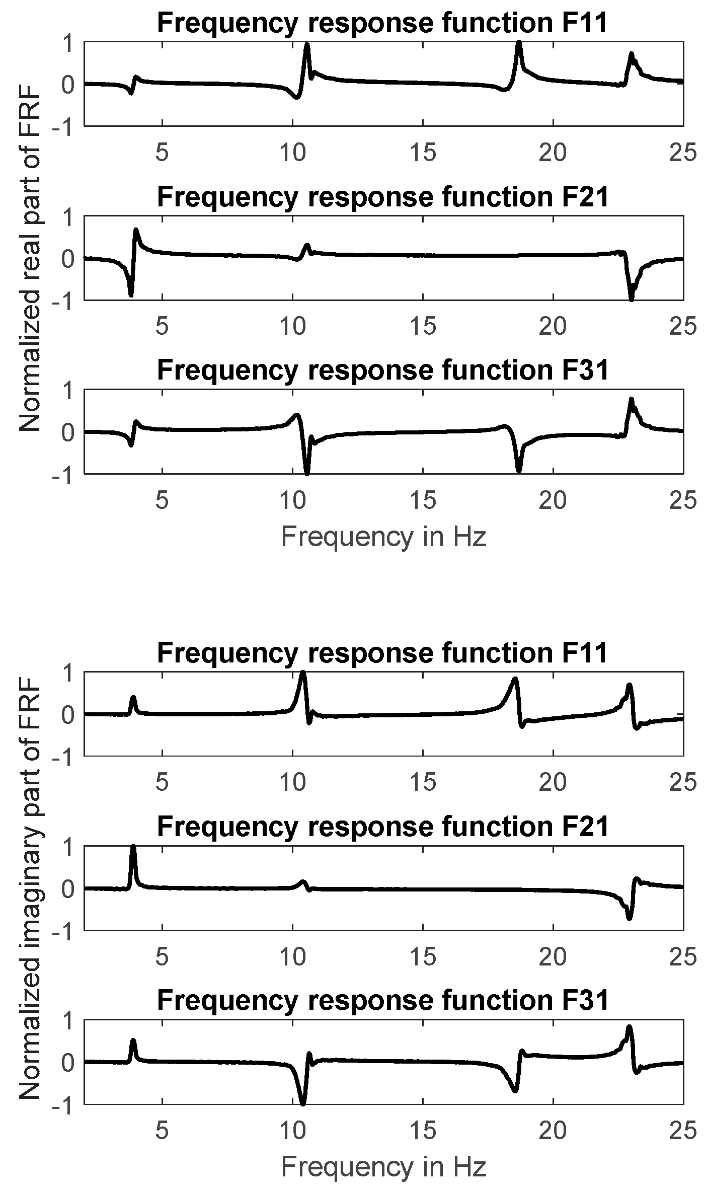

Table 1.
Physical parameter of frame structure.
| Parameter | Description | Value and Unit |
|---|---|---|
| Width cross section | 0.030 m | |
| Height cross section | 0.002 m | |
| Length of horizontal part of frame structure | 0.895 m | |
| Length of vertical part of frame structure | 0.010 m | |
| Horizontal position of 1st point mass | 0.224 m | |
| Horizontal position of 2nd point mass | 0.448 m | |
| Horizontal position of 3rd point mass | 0.671 m | |
| Density of frame structure material | 2700 kg/m3 | |
| Young's modulus of frame structure material | 79e9 N/m² | |
| Weight of mass at 1st point mass position | 0.158 kg | |
| Weight of mass at 2nd point mass position | 0.290 kg | |
| Weight of mass at 3rd point mass position | 0.158 kg |
Table 2.
Normalized magnitudes at resonance frequencies.
| fR / Hz | Left | Middle | Right |
|---|---|---|---|
| 3.87 | 1.00 | 1.98 | 1.27 |
| 10.5 | 1.00 | 0.14 | 0.99 |
| 18.7 | 1.00 | 0.04 | 0.84 |
| 23.0 | 1.00 | 0.75 | 1.07 |
Table 3.
Phase relations in grad at resonance frequencies.
| fR / Hz | Left | Middle | Right |
|---|---|---|---|
| 3.87 | 0.00 | -0.82 | -0.08 |
| 10.5 | 0.00 | -8.55 | -179 |
| 18.7 | 0.00 | -69.5 | 180 |
| 23.0 | 0.00 | -174 | 6.92 |
Table 4.
Modal assurance criteria values for measured mode shapes.
| Mode number | 1 | 2 | 3 | 4 |
|---|---|---|---|---|
| 1 | 1.00 | 0.00 | 0.00 | 0.04 |
| 2 | 0.00 | 1.00 | 0.98 | 0.01 |
| 3 | 0.00 | 0.98 | 1.00 | 0.01 |
| 4 | 0.04 | 0.01 | 0.01 | 1.00 |
Table 5.
Modal damping in resonance.
| Mode number | 1 | 2 | 3 | 4 |
|---|---|---|---|---|
| Modal Damping | 2.8% | 1.4% | 0.8% | 0.4% |
Table 6.
Peak magnitudes at resonance frequencies in m/s²/V.
| fR / Hz | Left | Middle | Right |
|---|---|---|---|
| 3.87 | 1.09 | 2.16 | 1.39 |
| 10.5 | 2.87 | 0.41 | 2.82 |
| 18.7 | 3.07 | 0.11 | 1.91 |
| 23.0 | 2.56 | 1.91 | 2.72 |
Table 7.
Natural frequencies for first three bending modes and first horizontal mode.
| Mode | Beding,1 | Bending,2 | Horizontal,1 | Bending,3 |
|---|---|---|---|---|
| f / Hz | 2.28 | 10.6 | 17.9 | 21.3 |
Disclaimer/Publisher’s Note: The statements, opinions and data contained in all publications are solely those of the individual author(s) and contributor(s) and not of MDPI and/or the editor(s). MDPI and/or the editor(s) disclaim responsibility for any injury to people or property resulting from any ideas, methods, instructions or products referred to in the content. |
© 2025 by the authors. Licensee MDPI, Basel, Switzerland. This article is an open access article distributed under the terms and conditions of the Creative Commons Attribution (CC BY) license (http://creativecommons.org/licenses/by/4.0/).
Copyright: This open access article is published under a Creative Commons CC BY 4.0 license, which permit the free download, distribution, and reuse, provided that the author and preprint are cited in any reuse.


