Submitted:
25 July 2025
Posted:
29 July 2025
You are already at the latest version
Abstract
The Zernike polynomials method is popular in the generation of atmospheric phase screen, but suffers from the high frequency components insufficiency. Hence, the higher terms of Zernike polynomials need to be calculated, creating new problems: computational inefficiency and numerical instability, their causes (calculating the Zernike radial polynomials with the direct method) and consequences are discussed and analyzed in detail in the following paper. Substituting the direct method with a recursive formula can solve these problems. Furthermore, four popular and excellent recursive methods are chosen, and their performances on phase screen generation are studied and discussed with respect to computational efficiency and numerical stability, respectively. The results shows an increase of 10-20 times in computational efficiency for phase screen generation and numerical stability maintained even for the thousands of terms arising from Zernike polynomials since the recursive radial formula is adopted.
Keywords:
phase screen
; atmospheric simulation
; zernike polynomials
; numerical stability
; recursive method
1. Introduction
When a light beam propagates through the atmosphere, it will be influenced by the turbulent effect that causes its wavefront to be disturbed, hence inducing the phenomena of light intensity scintillation, imaging distortion and beam drifting [1]. It is a big challenge in astronomical observation. As a consequence, the simulation of atmospheric turbulence provides a valuable technique to better understand these effects. The frozen flow hypothesis, also known as Taylor hypothesis [2], has shown that it is possible to simulate the turbulence effects with a thin screen on which the accumulated distorted wavefront is evaluated. In addition, the study of the atmospherically distorted wavefront is also closely associated with several other research fields, such as adaptive optics system debugging [3, 4], learning-based algorithms linked to atmospheric effects [5, 6], optical experiment simulations [7], etc.
Many methods have been proposed to generate the atmospheric phase screen [8-10]. The Zernike polynomials method is a popular method, first detailed by Roddier[10]. However, the Zernike polynomials method suffers from issues with high frequency components insufficiency, and the only solution is to calculate the higher orders of the Zernike polynomials as much as possible, which is numerically intense. This is especially true when generating a phase screen with a large aperture, thousands of terms are needed [11] in order to properly simulate the physical phenomena because a larger aperture corresponds to having a higher cut-off frequency in a diffraction-limited optical system. However, since the Zernike polynomials method is widely used for studies involving anisoplanatic turbulence simulations [12] and dynamic phase screen simulations [13, 14], it’s necessary to address the remaining issues first. The problems are computational inefficiency and numerical instability while numerically computing the values of Zernike polynomials. According to the Carbillet and Riccardi [11], Forbes [15] and Niu and Tian [16], using a recursive formula to calculate the Zernike radial polynomials is a possible solution. Moreover, it is worth discussing how the computational method of Zernike radial polynomials influences the phase screen generation.
In this paper, Section 2 details the generation of phase screen using the Zernike polynomials method and discusses the reasons and consequences of computational inefficiency and numerical instability. In order to solve these problems, four popular recursive radial formulas are introduced in Section 3 and presented in detail. Next, their performances in the generation of phase screen are experimented with and discussed in Section 4. Finally, a conclusion is provided in Section 5.
2. Theory and Problems
2.1. Atmospheric Phase Screen with Zernike Polynomials Method
An optical wavefront can be viewed as a two-dimensional function which can be decomposed into a linear combination of orthogonal bases. The Zernike polynomials have been offered such a set of bases that are orthogonal over a unit circle, and the mathematical expression of them under Noll’s definition[17] is as follows:
where
Equation(2) is the analytic expression of Zernike radial polynomials. Besides, n denotes the radial index number, and its repetition m is the azimuthal frequency. These indices must satisfy the following conditions: 0 ≤ m ≤ n and n − m = even, the transform relations between single index j to double indices n and m are detailed in[16].
As previously mentioned, a wavefront can be expressed as a linear combination of a series of Zernike polynomials since they are orthogonal with each other over the unit circle, its mathematical expression is written as:
where aj is the weighting coefficient of the j-th order of the Zernike polynomial Zj, and N corresponds to the maximum Zernike term used to generate the wavefront function. Besides, we summate equation(3) starts from j = 2 since the piston term(corresponds to j = 1 term in Zernike polynomials) does not contribute to the atmospheric screen. Additionally, for cases where the radius of aperture R is unequal to 1, the transform ρ = r/R can be made(r ranges from 0 to R), thereby ρ will be normalized within any given circle aperture size.
However, it is still ineffective to simulate the randomly distorted phase screen only by generating a series of Gaussian random numbers for coefficients aj(j = 2,3,...,N) for equation(3) since there exists a given covariance between them has to be taken into account, meaning the fact that Zernike polynomials are not statistically independent from each other[17]. The expression of covariance between any two Zernike coefficients under Kolmogorov spectrum consideration is given as[10, 17]:
where Kij is a factor given as:
where n,n′,m and m′ are the radial degrees and azimuthal frequencies of Zernike polynomials corresponding to aj and aj′. And δjj′ is a logical Kronecker symbol defined as:
where parity(j,j′) denotes whether the indexing number j and j′ have the same parity.
Then, the collection for the correlation of coefficients can be written as a covariance matrix where its elements are computed by equation(4):
and A is the vector of Zernike coefficients that is A = [a2,a3,...,aN]T.
Furthermore, correlated and random Zernike coefficients can be drawn from this covariance matrix. Decomposition through the Cholesky factorization method that is used by Nicholas Chimitt and Stanley H.Chan[12] was adopted in our work. Instead of the singular value decomposition(svd) method commonly used, since the covariance matrix C is a sparsely symmetric and positive definite matrix, a faster and more accurate programming operation will result if this strategy is taken. The Cholesky factorization is given as:
where L is a lower triangular matrix. Then creating a
Gaussian random vector B and
its elements are zeros indicating mean Gaussian random numbers with unit
variance. The transformed coefficient vector:
will be satisfied by E[AAT] = C. So far, a simple and rapid method can be utilized to draw random samples of inter-mode correlated Zernike coefficients.
The coefficients vector(9) therefore can then be substituted into equation(3) to generate the random atmospheric phase screen, which satisfies the statistical properties of Kolmogorov turbulence.
After all this preparation, equation(3) can then be written into numerical vector-matrix format for programming, which can be compactly written as:
where W is a column vector with elements evaluated within the aperture under linear indexing, the length of which is equal to the number of grid points on the aperture circle. Z can be expressed as Z = [Z2|Z3|...|ZN] while Z2,Z3 etc. which are column vectors with linear-indexed Zernike polynomials values on the aperture, and the length of each term is same as W.
2.2. Evaluation of The Generated Phase Screens
Calculating the structure function is a common method for confirming if performance of the generated phase screens satisfies the specified statistical property, it is computed by definition:
where "⟨...⟩" stands for the average value. Theoretically, for a good approximation to Kolmogorov turbulence, D(r) should follows:
where r = |r|.
In Figure 1, the
experiments are plotted with parameters: aperture radius R = 1m, Fried constant
r0 = 0.1, numbers of grid size(resolution) 256 and variant parameter
nmax, and transformation: N =  can
be applied to compute the total terms of Zernike polynomials used in
phase screen generation. The theoretical curve(black curve) was plotted from equation(12). As observed in Figure 1, ignoring the red color curves for a moment, the low frequency part of the experimental and theoretical values fit well, while the high frequency part of the experimental values is insufficient. However, as the number of terms of the Zernike polynomial increases (nmax from 10 up to 40), the high frequency components of experimental values approach the theoretical value curve. Roddier[10] pointed out that the result simulated by a few hundred terms of Zernike polynomials is satisfactory, of course, it is enough for long-range imaging scenarios. However, it will probably be necessary to use thousands of terms of polynomial to estimate the blurring effect induced by high-order aberrations when large aperture and astronomical imaging are taken into account. Besides, the experimental values of the red curves (dash-dot line for nmax = 50, solid line for nmax = 55) significantly deviate from the theoretical curve producing an abnormal phenomenon, which is due to the numerical instability in the calculation of high-order Zernike polynomials as detailed in the next section.
can
be applied to compute the total terms of Zernike polynomials used in
phase screen generation. The theoretical curve(black curve) was plotted from equation(12). As observed in Figure 1, ignoring the red color curves for a moment, the low frequency part of the experimental and theoretical values fit well, while the high frequency part of the experimental values is insufficient. However, as the number of terms of the Zernike polynomial increases (nmax from 10 up to 40), the high frequency components of experimental values approach the theoretical value curve. Roddier[10] pointed out that the result simulated by a few hundred terms of Zernike polynomials is satisfactory, of course, it is enough for long-range imaging scenarios. However, it will probably be necessary to use thousands of terms of polynomial to estimate the blurring effect induced by high-order aberrations when large aperture and astronomical imaging are taken into account. Besides, the experimental values of the red curves (dash-dot line for nmax = 50, solid line for nmax = 55) significantly deviate from the theoretical curve producing an abnormal phenomenon, which is due to the numerical instability in the calculation of high-order Zernike polynomials as detailed in the next section.In conclusion, the experimental phase structure functions indicate that the Zernike polynomial method has a problem: it is insufficient in high frequency components, using the terms of Zernike polynomials, as many as possible, to generate the phase screen is the only way to overcome while bringing two new challenges: (1) a corresponding increase in computation; and (2) the numerical instability issue existing in the calculation of high-order of Zernike polynomials.
2.3. Challenges in Computational Efficiency and Numerical Stability
In the previous section, equation(2) is denoted as the direct method for computation of Zernike radial polynomials. One drawback is that, as can be seen from the direct method, abundant computational requirements are needed since the equation(2) is heavily dependent on repeated factorial calculation and power series of radius ρ(by the way, it is an extensive vector for phase screen generation, e.g., with 51420 grid points within the aperture circle for 256 × 256 resolution screen). Therefore, the computational efficiency of the entire program suffers from the direct method; a simple experiment illustrating the issue is shown in Figure 2.
Figure 2 identifies the huge computational cost of elapsed CPU time for computing the Zernike radial polynomials using the direct method adopting the programming strategy provided earlier. Comparatively, in the left graph, the solid line represents the total runtime for executing the entire phase screen generation program, where the dash-dot line corresponds to the cost contributed by radial polynomials computed using
the direct method, and the right graph represents the proportion of computational assumption of the direct method over the entire program as a percentage, which are the results of the dash-dot line divided by the solid line for different color lines, respectively. Where in both graphs, the different color lines: red, blue, purple and black correspond to phase screens generated with resolution(Number of grid points) of 64 × 64,128 × 128,256 × 256,512 × 512, respectively.
The Left graph in Figure 2 shows that, for different color lines, solid lines and dash-dot lines are very close together, indicating the considerable time-demand that the direct method consumes for the entire program. Therefore, the right graph in Figure 2 is an illustration of quantification of the direct method influences the computational consumption for the whole program. As can be seen, the curves are almost over 85%. Moreover, for cases of generation of the exact screen(high values of nmax), the value of percentage proportion is about 93%(excepting 512×512 resolution, which still higher than 85%). Thus, we believe the results in Figure 2 proved the direct method is the root cause of the computational problem for the Zernike method. It is clear that, based on the right graph, the curves stabilize gradually and separate distinctly after nmax exceeds 30, and higher resolution corresponds to a lower proportion. The results indicate that the computational efficiency in phase screen generation suffers more from secondary operations(e.g. Zernike angular polynomials, decomposition of covariance matrix, and matrix manipulation, etc.) as screen resolution increases. However, their computational consumption still can not be comparable with the radial polynomials.
Further, another problem in equation(2) remains. It is
simple to verify that , which is contributes to
the numerical crumble in Zernike radial polynomials, because the magnitude of
coefficients of Rnm(ρ) reaches up to 100.7n[15], this means that, for cases of equation(2)
concerning high-index number n and the evaluation of radius ρ close to 1, where
heavy cancellation in decimal parts happens when the summation of an enormous
number will eventually shrink to the value close to 1, example for numerical
catastrophe on radial polynomials and phase screen can be seen in Figure 3. Therefore, it’s no longer possible to
guarantee numerical stability for computing radial functions with direct method
once index n exceeds 40(calculate with double precision)[18], resulting in problems in the generation of
higher precision phase screen using the Zernike method.
Figure 3 illustrates the numerical instability problem when using Zernike polynomials for phase screen generation. The left graph shows that Zernike radial polynomials computed using the direct method encountered critical numerical instability due to the aforementioned reason. The right one depicts the phase screen generated by the direct method for radial polynomials computation, of which ”burr effects” occurred at the edge of the screen which corresponded to the numerical instability phenomenon where values of radius ρ approximate to 1. Where the oscillated values result in the structure function deviating strongly from the theoretical curve, as shown in Figure 1, the red curves.
In summary, the Zernike polynomials method uses the direct method, equation(2), when calculating radial polynomials, resulting in computational inefficiency and numerical instability problems in the generation of phase screens. Accordingly, recursive radial formulas were recommended to eliminate the drawbacks of the direct method for calculating Zernike radial polynomials[15, 19]. However, the performance of radial recursive formulas in the study of phase screen generation still needs to be completed.
3. Recursive Methods of Zernike Radial Polynomials
Compared with the direct radial method, the recursive formula accelerates the computation speed by reducing repetitive operations, i.e., factorials and vector multiplication. It prompts robust computation by avoiding the heavy cancellation of digital numbers. In this section, four different recursive formulas are selected and introduced: Barmak’s method[20], q-recursive method[19], Prata’s method[21] and Kintner’s method[22].
3.1. Barmak’s Method
Barmak Hornarvar Shakibaei and Raveendran Paramesran[20] proposed the following recurrence expression, denoted as Barmak’s method, deriving based on the Chebyshev polynomials of the second kind. The formula is given as:
With the initial value and Rmn
(ρ) = 0 when n < m, it is possible to use equation(13) to generate
the necessary terms. Further, compared to the other three recursive formulas
discussed below, Barmak’s formula is the only method independent on the
computation of coefficients.
3.2. q-Recursive Method
Chong et al.[19] proposed the q-recursive method for fast computation of Zernike radial polynomials. The q-recursive method uses radial polynomials with fixed index n and higher index m to derive the radial polynomial with a lower index m. The recurrence formula is given as:
where the coefficients H1,H2, and H3 are given by
Formula(14) is not applicable in cases where n − m = 0 and n − m = 2, for these exceptional cases, the following recurrence relations can be applied:
Using the computational strategy above, instead of the direct method, in cases n−m = 0 and n−m = 2, boosting computational speed by avoiding the repeating computation of the power series of radius and calculation of coefficients. Besides, once the initial values, Rmn (ρ) with cases n − m ≤ 2, are calculated, then the remaining polynomials can be recursively computed using equation(14). Furthermore, n-th order polynomials can be computed individually since they are independent of the other n-th order polynomials. Therefore, the q-recursive method is ideal with regards to parallel computation in programming[19].
3.3. Prata’s Method
Prata[21] derived a three-term recurrence relation for calculating the Zernike radial polynomials, given as:
where the coefficients L1 and L2 are defined as:
With the initial valuesR00 (ρ) = 1 and Rmn (ρ) = 1 when n < m, which is the same approach as Barmak’s method, it is also possible to recursively derive all terms of radial polynomials that enable the higher order radial polynomials to be derived from the linear combination of lower order polynomials.
3.4. Kintner’s Method
Kintner[22] derived a three-term recurrence relation, based on the recursive properties of Jacobi polynomials, to calculate the higher order Zernike radial polynomials with lower degree n of a fixed azimuthal order m, which is given as:
where the coefficients K1,K2,K3 and K4 are given by
Similarly, formula(19) also breaks down in cases of n−m = 0 and n−m = 2, which is similar to the q-recursive method. Therefore, Chong et al.[19] modified Kintner’s method by applying equation(16) cases where n − m ≤ 2.
Thus, the four popular recursive radial computation methods are introduced. In the next section, their performance in applying phase screen generation will be studied and discussed.
4. Performance and Discussion
In this section, we will assess the performance of four recursive methods for phase screen generation in computational efficiency and numerical stability. Finally, the optimal results for both problems are reached.
4.1. Computational Efficiency of Phase Screen Generation with Different Recursive Methods
In this part, for experimentally studying of phase screen generation using the four different recursive methods to determine the performance of computational efficiency. This process utilized four variant sizes of screens(64×64,128×128,256×256,512×512), and the maximum terms of the Zernike polynomials (N) used in equation(3) are computed from 231 to 5151(corresponding to nmax values from 20 to 100). As shown in Table 1, and comparing these values with the results in Figure 2, we can conclude that operating speed increases 10-20 times for the phase screen generated program after substituting the direct method by recursive method for the computation of Zernike radial polynomials. The subtle and not tremendous differences in CPU elapsed time being existed for variant recursive methods which are also shown in Table 1.
According to Table 1, Barmak’s method performs well for situations with low resolution(64×64, 128× 128) because of MATLAB is better at computing matrix operations. We can observe from equation(13) that the formula depends only on three radial polynomial terms to derive the new term without the tedious computation of coefficients. However, it also means that Barmak’s method suffers heavier vector operations, therefore its effectiveness decreases with increasing screen resolution(256 × 256, 512 × 512).
Examining the rest of the recursive methods. They all consist of a three-term formula but suffered more from the expensive computation of coefficients than Barmak’s method. As shown in Table 1, Prata’s method performs faster in circumstances of low resolution nmax ≤ 256×256 since the coefficients computation is straightforward. Nevertheless, differences are reduced between the three methods with the increasing data matrix size (relates to parameters: resolution and nmax) where vector operation takes up the majority of computing consumption instead of coefficients calculation. However, both qrecursive and Kintner’s methods are more stable with respect to numerical computation, as detailed in the following section. Then, they all perform better with increasing screen resolution compared to Barmak’s method.
4.2. Numerical Stability of Different Recursive Methods
As we have verified, radial polynomials computed by direct method is the root cause of the numerical crumble problem. Thereby, to quantitatively study the numerical problem in recursive radial methods, Mohammed Sadeq Al-Rawi[18] defined a quality-factor for verifying the numerical stability of orthogonal polynomials which has been used to show that, in Zernike radial polynomials, where the numerical instability starts: nmax ≥ 40 for direct method, nmax ≥ 80 for Prata’s method, but heavy numerical crumble problem does not appears in Kintner’s method or q-recursive method even when nmax ≥ 250. Furthermore, according to G.A.Papakostas et al.[23, 24], the numerical error in Zernike radial recursive computation methods occurs from ill-posed subtraction and overflow. In other words, the subtraction between two similar numbers and a tremendous number of values divided by a small number in the computation of coefficients are the causes of numerical instability in recursive formulas, instead of vector operations. Therefore, Barmak’s method, equation(13), can be considered without suffering from heavy numerical error since its computational equation is dependent only on vector operations, which without the illposed and overflow problems mentioned above, theoretically means that Barmak’s method is the most stable formula for recursive computation of Zernike radial polynomials.
Nevertheless, for thousands order of Zernike polynomials in turbulence simulation, their weighting coefficients aj are extremely small(the random numbers with zero means and about 10−5 variances). Further problems still need to be solved: Will the numerical quality of the phase screen itself be destroyed by such small coefficients multiplied by the unstable polynomials? Which is done to verify the instability effect on the phase screen instead of on the polynomials. Therefore, we define a Quality-factor ”Q” by computation as follows:
where W is the mean value of over the aperture. According to the theory of mean-square wavefront aberration of Zernike-generated screen[25], the values of ”Q” should be theoretically close to zero if numerical instability does not exist. Alternatively, the values of ”Q” should deviate from zeros in circumstances where numerical problems arise.
Figure 4 illustrates the value of Quality-factor ”Q” changes with the increase of nmax(corresponds N ranges from 23 to 7381), the data for q-recursive and Kintner’s method are not plotted on the graph since their curves are coincident with Barmak’s method curve. Moreover, Figure 4 indicates that numerical catastrophe has been happening on the phase screens, where the values of Quality-factor ”Q” dramatically increase for radial polynomials computed by the direct method and Prata’s method where nmax ≥ 40 and nmax ≥ 80, respectively. This coincides with previous analyses in the theory of numerical crumble in Zernike radial polynomials. Hence, we can conclude that the numerical quality of phase screen is strongly correlated to the numerical stability of Zernike radial polynomials. Combined with results from the radial polynomials discussed previously, we have proved that Barmak’s method, q-recursive, Kintner’s, and Prata’s method(nmax ≤ 80) are all numerically stable in the application of phase screen generation.
4.3. Discussion
The results, shown in Table.1 was obtained using Matlab 2020a with default calculation precision(16 significant digits). As previously mentioned, Prata’s method usually performs well in computational speed but not in numerical stability when nmax ≥ 80. Additionally, we can conclude that with the increase in screen resolution(even for a resolution higher than 512×512), Barmak’s method is not recommended with respect to computational efficiency. The differences in computational speed(measured in CPU elapsed time) between the other three methods(q-recursive, Prata and Kintner) will not be separated clearly since the majority gradually become vector operations instead of coefficients computation. Where Barmak’s method is recommended for low resolution situations(e.g. 64 × 64,128 × 128) and q-recursive or Kintner’s method is recommended for high resolution situations(e.g., 256×256,512×512 or larger cases) both with respect to efficiency and stability. In addition, the results shown in Table 1 are measured using CPU elapsed time rather than actual CPU running time. Therefore, perhaps the program will perform faster by adopting the q-recursive method in a high-performance machine since the q-recursive method can work for calculating the radial polynomials with parallel computation in programming[19].
Further, let us combine the results shown at Section 2 and Section 4. On the one hand, to evaluating the increase in computing speed, focusing on Figure 2 and Table 1, supposing that the direct method were substituted with Prata’s method, when nmax = 40 , we can estimate that there will be an increase from 10 to 20 times for the efficiency of the overall program for phase screen generation. Alternatively, adopting the recursive radial computing method to remove the coefficient explosion issue for the direct method, means that an more exact phase screen can stably generated, corresponding to cases where nmax ≥ 40 at which point the radial polynomials computed by direct method begin to oscillate.
By the way, employing the programming strategy from equation(10) for phase screen generation with respect to high precision and resolution, is where the storage challenge arises. E.g., a phase screen with size 256 × 256 and maximum terms of Zernike polynomials jmax = 3321(corresponds nmax = 80), with double precision arithmetic, memory capacity for saving matrix Z is up to 1.3GB. Hence, it can be derived that about 83GB memory capacity is necessary for saving matrix Z for a screen of size 4096 × 4096. Therefore, the Zernike method is not feasible for a low-performance computer to simultaneously generate a phase screen with both high resolution and precision. Hence, a method proposed by Cressida M. Harding et al.[26] can be referenced, in which the Zernike method first generates a screen with low resolution but high precision, then the interpolations are implemented to increase the resolution. In other words, combining the Zernike method and the fractal method. We can not only mitigate the effects of random errors in the fractal method if we start interpolations on a theoretically precise screen, but also avoiding the large-scale matrix operation present in the Zernike polynomials method.
5. Conclusions
This paper discusses computational inefficiency and numerical instability problems found in phase screen generation using the Zernike polynomials method, while the root cause is computing radial polynomials via direct method. As a solution, recursive radial methods are introduced to substitute for the direct method in the calculation of Zernike radial polynomials. Experiments show that for phase screen generation, an increase of 10 to 20 times occurs with computational efficiency for a recursive radial method adopted as a substitute for the direct method. Moreover, with suitable recursive methods for different cases, improvements in numerical stability can be guaranteed also even for thousands of terms for a Zernike polynomials generated screen. Thus, by adopting such a programming strategy, a more efficient and precise phase screen generation program can be implemented effectively improving its application to atmospheric turbulence-related work.
Funding
Project supported by the National Natural Science Foundation of China (Grant No.42004134) Shanxi Basic Research Program (Grant No. 202303021221051).
Acknowledgements
The authors would like thank Dr. Maurice Lineman, a Canadian expatriate working in China, for editing the paper for English grammar and contextual understanding.
Conflicts of Interest
The authors declare no conflicts of interest.
References
- Robert, K. Tyson. Principles of Adaptive Optics(Chinese version), pages 21–22. National Defense Industry Press, Beijing, China, 3-rd edition, 2017.
- G. I. Taylor. The Spectrum of Turbulence. Proceedings of the Royal Society of London. Series A Mathematical and Physical Sciences, 164(919):476–490, 1938.
- Peng Jia, Dongmei Cai, Dong Wang, and Alastair Basden. Simulation of atmospheric turbulence phase screen for large telescope and optical interferometer. Monthly Notices of the Royal Astronomical Society, 2015, 447, 3467–3474. [CrossRef]
- Sandrine Thomas. A simple turbulence simulator for adaptive optics. In SPIE Astronomical Telescopes + Instrumentation, page 766, USA, October 2004.
- Peng Jia, Weihua Wang, Runyu Ning, and Xiaolei Xue. Digital twin of atmospheric turbulence phase screens based on deep neural networks. Optics Express, 2022, 30, 21362. [CrossRef] [PubMed]
- Qi-Wei Xu, Pei-Pei Wang, Zhen-Jia Zeng, Ze-Bin Huang, Xin-Xing Zhou, Jun-Min Liu, Ying Li, ShuQing Chen, and Dian-Yuan Fan. Extracting atmospheric turbulence phase using deep convolutional neural network. Acta Physica Sinica, 2020, 69, 014209.
- S. M. Zhao, J. Leach, L. Y. Gong, J. Ding, and B. Y. Zheng. Aberration corrections for free-space optical communications in atmosphere turbulence using orbital angular momentum states. Optics Express, 2012, 20, 452. [CrossRef] [PubMed]
- Benjamin, L. McGlamery. Conputer simulation studies of compensation of turbulence degraded images. Image Processing, pages 225–233, 1976.
- Huili Zhai, Bulan Wang, Jiankun Zhang, and Anhong Dang. Fractal phase screen generation algorithm for atmospheric turbulence. Applied Optics, 2015, 54, 4023.
- Nicolas A. Roddier. Atmospheric wavefront simulation using Zernike polynomials. Optical Engineering, 1990, 29, 1174. [CrossRef]
- Marcel Carbillet and Armando Riccardi. Numerical modeling of atmospherically perturbed phase screens: New solutions for classical fast Fourier transform and Zernike methods. Applied Optics, 49(31):G47, November 2010.
- Nicholas Chimitt and Stanley H. Chan. Simulating Anisoplanatic Turbulence by Sampling Intermodal and Spatially Correlated Zernike Coefficients. In 2020 IEEE INTERNATIONAL CONFERENCE ON COMPUTATIONAL PHOTOGRAPHY (ICCP), number arXiv:2004.11210. arXiv, June APR 24-26, 2020.
- Christopher, C. Wilcox. Performance of a flexible optical aberration generator. Optical Engineering, 50(11):116601, November 2011.
- Esdras Anzuola and Szymon Gladysz. Modeling dynamic atmospheric turbulence using temporal spectra and Karhunen–Loève decomposition. Optical Engineering, 56(07):1, March 2017.
- G. W. Forbes. Robust and fast computation for the polynomials of optics. Optics Express, 18(13):13851, June 2010.
- Kuo Niu and Chao Tian. Zernike polynomials and their applications. Journal of Optics, 24(12):123001, December 2022.
- Robert, J. Noll. Zernike polynomials and atmospheric turbulence. Journal of the Optical Society of America, 66(3):207, March 1976.
- Mohammed Sadeq Al-Rawi. Numerical Stability Quality-Factor for Orthogonal Polynomials: Zernike Radial Polynomials Case Study. In Image Analysis and Recognition, volume 7950, pages 676–686. June 2013.
- Chee-Way Chong, P. Raveendran, and R. Mukundan. A comparative analysis of algorithms for fast computation of Zernike moments. Pattern Recognition, 2003, 36, 731–742. [CrossRef]
- Barmak Honarvar Shakibaei and Raveendran Paramesran. Recursive formula to compute Zernike radial polynomials. Optics Letters, 2013, 38, 2487. [CrossRef] [PubMed]
- Aluizio Prata and W. V. T. Rusch. Algorithm for computation of Zernike polynomials expansion coefficients. Applied Optics, 1989, 28, 749. [CrossRef] [PubMed]
- Eric, C. Kintner. On the Mathematical Properties of the Zernike Polynomials. Optica Acta: International Journal of Optics, 23(8):679–680, August 1976.
- G.A. Papakostas, Y.S. G.A. Papakostas, Y.S. Boutalis, C.N. Papaodysseus, and D.K. Fragoulis. Numerical error analysis in Zernike moments computation. Image and Vision Computing, 24(9):960–969, September 2006.
- G.A. Papakostas, Y.S. Boutalis, C.N. Papaodysseus, and D.K. Fragoulis. Numerical stability of fast computation algorithms of Zernike moments. Applied Mathematics and Computation, 2008, 195, 326–345. [CrossRef]
- Jason, D. Schmidt. Numerical Simulation of Optical Wave Propagation with examples in MATLAB, pages 76–77. SPIE PRESS, Bellingham, Washington, USA, 2010.
- Cressida M. Harding, Rachel A. Johnston, and Richard G. Lane. Fast simulation of a kolmogorov phase screen. Applied Optics, 1999, 38, 2161. [CrossRef] [PubMed]
Figure 1.
Structure function compared between theoretical and experimental results with parameters D/r0 = 20 for atmospheric phase screens with Kolmogorov statistics, averaging 1000 screens for each curve.
Figure 1.
Structure function compared between theoretical and experimental results with parameters D/r0 = 20 for atmospheric phase screens with Kolmogorov statistics, averaging 1000 screens for each curve.
Figure 2.
Left: CPU elapsed time of the entire program(solid line) and direct method(dash-dot line). Right: the proportion of elapsed time of direct method over the entire program(The program was executed by a laptop with Intel-1240P CPU and 4800MHZ memory, averaging 300 iterations, performed on Matlab 2020a).
Figure 3.
Left: Zernike radial polynomials computed by direct method with n = 46,m = 0. Right: Phase screen generated by Zernike polynomials method with direct method(simulated with parameters: r0 = 0.1,D = 2(m),nmax = 50).
Figure 3.
Left: Zernike radial polynomials computed by direct method with n = 46,m = 0. Right: Phase screen generated by Zernike polynomials method with direct method(simulated with parameters: r0 = 0.1,D = 2(m),nmax = 50).
Figure 4.
The values of Quality-factor ”Q” in phase screen changes with respect to nmax, the radial polynomials are computed with three different recursive methods, experimented with parameters: 256× 256 resolution, D/r0 = 20, averaging 300 iterations.
Figure 4.
The values of Quality-factor ”Q” in phase screen changes with respect to nmax, the radial polynomials are computed with three different recursive methods, experimented with parameters: 256× 256 resolution, D/r0 = 20, averaging 300 iterations.
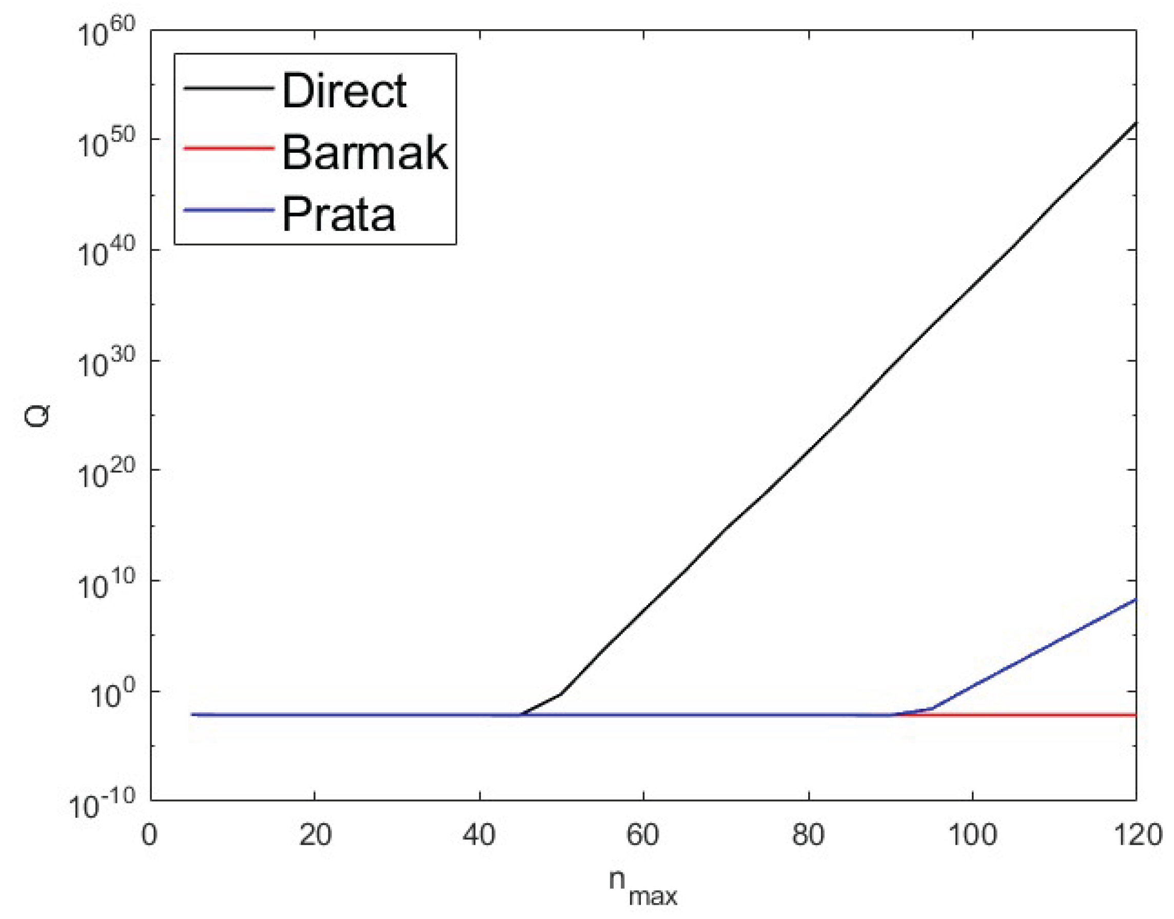

Table 1.
This is a table. Tables should be placed in the main text near to the first time they are cited.
Table 1.
This is a table. Tables should be placed in the main text near to the first time they are cited.
| nmax | Barmak’s | q-recursive | Prata’s | Kintner’s |
| method | method | method | method | |
| (a) 64 × 64 resolution 20 |
0.0188 | 0.0287 | 0.0142 | 0.0295 |
| 40 | 0.0959 | 0.1469 | 0.0883 | 0.1559 |
| 60 | 0.3556 | 0.4786 | 0.3474 | 0.5001 |
| 80 | 0.9323 | 1.1018 | 0.9153 | 1.1492 |
| 100 | 2.0232 | 2.2256 | 1.9924 | 2.3105 |
| (b) 128 × 128 resolution 20 |
0.0881 | 0.0902 | 0.0757 | 0.0980 |
| 40 | 0.3095 | 0.3356 | 0.2916 | 0.3723 |
| 60 | 0.7716 | 0.8674 | 0.7956 | 0.9589 |
| 80 | 1.9233 | 2.0885 | 2.0042 | 2.2449 |
| 100 | 4.1382 | 4.3408 | 4.2708 | 4.6017 |
| (c) 264 × 264 resolution 20 |
0.2909 | 0.2907 | 0.2858 | 0.3028 |
| 40 | 1.1555 | 1.1232 | 1.0904 | 1.1513 |
| 60 | 2.8843 | 2.7611 | 2.7011 | 2.8290 |
| 80 | 5.5887 | 5.3755 | 5.2905 | 5.4948 |
| 100 | 9.8839 | 9.5431 | 9.4223 | 9.7540 |
| (d) 512 × 512 resolution 20 |
1.6054 | 1.6578 | 1.5208 | 1.5549 |
| 40 | 6.5728 | 6.1043 | 5.5739 | 5.5705 |
| 60 | 15.6108 | 13.6742 | 12.7198 | 12.6816 |
| 80 | 28.6644 | 24.4980 | 22.9985 | 22.8596 |
| 100 | 51.4420 | 44.4752 | 42.0310 | 41.8682 |
Disclaimer/Publisher’s Note: The statements, opinions and data contained in all publications are solely those of the individual author(s) and contributor(s) and not of MDPI and/or the editor(s). MDPI and/or the editor(s) disclaim responsibility for any injury to people or property resulting from any ideas, methods, instructions or products referred to in the content. |
© 2025 by the authors. Licensee MDPI, Basel, Switzerland. This article is an open access article distributed under the terms and conditions of the Creative Commons Attribution (CC BY) license (http://creativecommons.org/licenses/by/4.0/).
Copyright: This open access article is published under a Creative Commons CC BY 4.0 license, which permit the free download, distribution, and reuse, provided that the author and preprint are cited in any reuse.


