
Submitted:
27 July 2025
Posted:
28 July 2025
You are already at the latest version
Abstract
Accurate prediction of extreme rainfall events during the Indian Summer Monsoon is critical for disaster preparedness and mitigation. This study evaluates the performance of two operational numerical weather prediction models, a high resolution version of Global Forecast System (GFS T1534) and the control member of the Met Office Global and Regional Ensemble Prediction System -Global (MOGREPS-G) in forecasting such events over the Indian region during the JJAS seasons from 2020 to 2023. Results show that both models tend to underestimate the mean and variability of rainfall, with GFS T1534 represents the mean and correlation better while MOGREPS-G represents the variability better over the Indian Landmass. Further a statistics based extreme rainfall threshold (50 mm/day) is fixed to compute the skill scores including Probability of Detection (POD), False Alarm Rate (FAR), and Bias. GFS T1534 shows moderate POD values but is limited by high FAR and underestimation biases. In contrast, MOGREPS-G displays higher POD at shorter lead times but suffers from elevated FAR and a strong over-forecasting tendency, particularly beyond 24 hours. The findings highlight strengths and limitations of both models in context of their operational use in extreme rainfall forecasting and early warning systems in India.
Keywords:
forecast skill
; extreme rainfall
; global forecast system
1. Introduction
The rise of extreme rainfall in different parts of the globe is well documented and reported by many previous studies [1,2,3,4,5] and mainly attributed this as a consequence of global warming. The wet regions in the tropics are getting wetter and dry regions are getting drier [6]. The extreme events also have various social, economic and environmental impacts [7]. Additionally extreme events demand preparedness for emergency response in different sectors including health sector [8]. A recent study reported that extreme rainfall reduces worldwide macroeconomic growth rates which in turn slows down the global economy [9]. In this rising trend of extreme rainfall events India is not an exception. Many previous studies have reported a significant rise in extreme rainfall events over Indian landmass [10,11,12,13]. The number of wet days with rainfall over 99th percentile is increasing over Indian region [14]. Additionally, there is also a significant rise in the intensity of rainfall over Indian landmass [15]. Another recent study highlighted that the widespread extreme rainfall rose to three-fold over central Indian region [16].
Keeping the socio-economic impact in mind the accurate prediction of these events is the need for the hour. Past studies highlighted that extreme rainfall is generally underestimated by current-generation climate models. Climate models tend to underestimate the frequency and intensity of extreme rainfall events [17,18]. A high resolution Global Forecast System (GFS T1534) for short and Medium range prediction is being implemented by the Indian Institute of Tropical Meteorology for operational requirements of Indian Meteorological Department (IMD). This model shows reasonable skill to capture broader structure of rainfall probability distribution functions [19]. It was also reported that UK Met Office Global and Regional Ensemble Prediction System (MOGREPS) shows better skill than the Global Ensemble Forecast System (NGEFS) of the National Centre for Medium Range Weather Forecasting (NCMRWF) across different rainfall threshold over Indian region [20]. Therefore, in this study we aim to evaluate the fidelity of GFS T1534 and MOGREPS-G in forecasting extreme rainfall events during JJAS season for the period 2020 to 2023. By comparing the predictions of extreme rainfall events from these two models, we aim to assess their accuracy and reliability. This evaluation will help us understand the strengths and limitations of each model in forecasting extreme rainfall events, ultimately contributing to improved weather prediction and risk management.
2. Materials and Methods
2.1. Model Description
The Global Forecast System (GFS) is a spectral model with 1534 triangular truncation and a horizontal resolution of around 12.5 km. It has c. The model is adopted from the NCEP and based on version 14 of GFS. It has a two-time level, semi-implicit, semi-Lagrangian discretization approach based dynamical core [21]. It uses the revised simplified Arakawa–Schubert (RSAS) convective parameterization scheme and mass-flux-based SAS shallow convection scheme [22]. For microphysics, it uses Zhao–Carr microphysics parameterization scheme [23]. This model is operationally used for short-range prediction in India [20]. The initial condition for the model run is generated by NCMRWF using ensemble Kalman filter (EnKF) component of hybrid global data assimilation system (GDAS) [24]. The model run is carried out at the Mihir HPC system of NCMRWF, New Delhi under the Ministry of Earth Sciences.
The Met Office Global and Regional Ensemble Prediction System-Global (MOGREPS-G) is a high-resolution (≈ 20 km) ensemble forecasting system for medium-range weather predictions [25]. It is a critical component of the UK Met Office’s numerical weather prediction (NWP) suite, providing both standalone global forecasts as well as the boundary conditions for nested regional models such as MOGREPS-UK. MOGREPS-G is a fully coupled to a quarter-degree ocean model, enabling two-way interaction between atmosphere and ocean. The model grid is based on an Arakawa A configuration, with equirectangular projection and a nominal resolution of N640. MOGREPS-G has 70 vertical levels extending up to 80Km altitude. Vertical levels are defined by height above ground as well as pressure levels, supporting a wide range of meteorological diagnostics. The MOGREPS-G uses a mass-flux convection scheme [26]. The microphysics used is a single-moment scheme [27] with extensive modifications [28]. MOGREPS-G provides forecasts up to 10 days and 6 hours (T+252). In this study, we have exclusively utilized the control simulation.
2.2. Data and Methodologies
To evaluate the model rainfall forecast we have used a high resolution gridded data set from IMD-GPM. IMD-GPM rainfall data is created by merging Global Precipitation Measurement (GPM) data with available rain gauge observations from Indian Meteorological department, and is available at resolution [29].
To evaluate the model forecast we have used statistical techniques such as mean, standard deviation, percentile analysis. Furthermore, to assess the forecast skill of the models, standard verification metrics including the Probability of Detection (POD), False Alarm Rate (FAR), and Bias Score are computed [30]. These skill scores are derived from a 2×2 contingency table constructed using observed and forecasted events, categorized as hits (a), false alarms (b), misses (c), and correct negatives (d). The POD represents the proportion of correctly forecasted ‘yes’ events relative to the total number of observed ‘yes’ events. The POD can range from 0 to 1 with 1 being the perfect score. It is calculated as,
The FAR shows the ratio of forecasted ‘yes’ events that did not occur. It also ranges from 0 to 1 with 0 being the ideal score and is calculated as follows,
Subsequently, the Bias score is a metric that calculates the ratio of forecasted ‘yes’ to the observed ‘yes’ occurrences. The perfect score is 1 while a score of < 1 (> 1) indicates under forecasting (over forecasting). It is calculated as,
3. Results and Discussion
It is important to recognize that extreme rainfall events are characterized by anomalously large deviations from the climatological mean rainfall. Therefore, understanding the ability of numerical weather prediction models to realistically simulate the mean rainfall distribution is a critical step before evaluating their skill in forecasting extremes. An accurate representation of the seasonal mean rainfall is essential, as systematic biases in the mean field can influence the reliability of extreme event simulations and forecasts.
Figure 1 illustrates the spatial distribution of the mean Indian Summer Monsoon (JJAS) rainfall as simulated by the two models under consideration (GFS T1534 and MOGREPS-G) at lead times of up to three days. Both models tend to underestimate the mean rainfall over most parts of the Indian region, with GFS T1534 showing relatively better agreement with observations over the Indian landmass. On the other hand MOGREPS-G appears to capture the mean rainfall more realistically over the Bay of Bengal region compared to GFS T1534.
To quantify the models’ performance in simulating mean rainfall patterns, spatial correlation analysis was conducted between the model-simulated and observed rainfall fields, as illustrated in Figure 2. The spatial correlation provides an overall measure of pattern agreement and is a key diagnostic in assessing model fidelity. Results indicate that the GFS T1534 exhibits positive spatial correlation with observations, with values reaching up to 0.5 at 24hr lead. However the correlation values are reducing with increasing lead time. On the other hand, the correlation coefficient between observation and MOGREPS-G is similar to that of with GFS T1534 at 24hr lead time but reduces drastically with increase of lead time and even becoming slight negative at 48hr and 72hr lead time in some of the region.
Another important statistical measure relevant to the assessment of extreme rainfall is the standard deviation, which quantifies the variability or fluctuation of rainfall from the mean. The standard deviation of JJAS rainfall over Indian region is illustrated in Figure 3. It can be seen that the standard deviation is underestimated by both the model implying a limited ability to reproduce the observed rainfall variability. The magnitude of underestimation is even more in GFS T1534 specially over Central India, North east and Bay of Bengal region. It should also be noted that MOGREPS-G overestimates the standard deviation in some parts of North East India. This underestimation of standard deviation indicates models inability to produce observed variability.
To investigate the prediction of extreme rainfall events we have fixed the threshold of extreme rainfall statistically by using percentile values. Figure 4 shows the spatial distribution of 95th percentile values from model and observation over Indian region. Figure 4 demonstrate that both models underestimate the 95th percentile threshold over large part of Indian Landmass. This underestimation increases with increase in lead time. The simulation by MOGREPS-G over Western Ghats, North East India is quite close to the observation. Furthermore both model underestimates the 95th percentile threshold quite a bit over Bay of Bengal, however comparatively MOGREPs-G is able to simulate spatial structure close to observation.
It should also be noted that in most of the central Indian region the threshold of 95th percentile is ranging between 30–50 mm/day, while only over western ghats and some parts of North East India the threshold exceeds over 80 mm/day. Hence, for our study we define extreme as rainfall over 50 mm/day. One of the important metric to evaluate in the context of extreme rainfall is R50 days, which denotes number of days with rainfall over 50 mm/day. Figure 5 shows the spatial pattern of R50 days over Indian region derived from Observation and models. It can be seen from observation (Figure 5a) that most of the central Indian region the magnitude of R50 days during our period of study (2020–2023) is between 20–40 days whereas in wester ghats and part of Northeast region is it going above 70 days. The number of R50 days simulated by GFS T1534 (Figure 5b–d) quite reasonable over the western ghats and parts of North east India, but underestimated very much over the Central Indian region at all lead times.
On the other hand the number of R50 days simulated by MOGREPS-G is much closer to the observation except some overestimation at western ghats and parts of North east India. We have also computed spatial pattern of R150 days following extreme rainfall threshold used by the past studies [11,12,17]. Result is shown in Figure 6. It can be seen that the number of R150 days are very small in models as well as observation, reaching up to 3–4 days over major parts of Indian landmass. This also strengthens the reasoning for defining extreme rainfall threshold as 50mm/day for this study. It is interesting to note that while GFS T1534 is underestimating the number of R150 days, MOGREPS-G found to be overestimate R150 days over parts of Central Indian region, Himalayan foothills region and the overestimation increases with the lead days.
To comprehensively assess the capability of the models in forecasting extreme rainfall events, skill scores such as the Probability of Detection (POD), False Alarm Rate (FAR), and Bias Score were computed. These categorical verification metrics are essential in quantifying the ability of a model to correctly identify extreme events, while also accounting for false alarms and systemic biases. In this analysis, extreme rainfall events are defined as instances where daily accumulated rainfall exceeds 50 mm/day. Figure 7 presents the spatial distribution of POD across the Indian region for both models at various lead times. The POD values for the GFS T1534 model at 24-hour lead time range from 0.3 to 0.7 across several key monsoonal zones, including Central India, Northwest India, Northeast India, and the Western Ghats. Among these, the Western Ghats exhibit the highest POD values, indicating a relatively higher model skill in capturing extreme events in this region.
However, a consistent decline in POD values is observed with increasing forecast lead time, reflecting a typical reduction in predictive skill at longer leads. In contrast, MOGREPS-G demonstrates generally higher POD values than GFS T1534 at the 24-hour lead time, particularly over Central India and Himalayan foothills region, suggesting better predictability at 24hr lead. Surprisingly, the model’s skill deteriorates markedly with lead time. At 48 and 72 hours, POD values decline substantially, with values dropping below 0.2 over large parts of the Central Indian region at 72 hours lead.
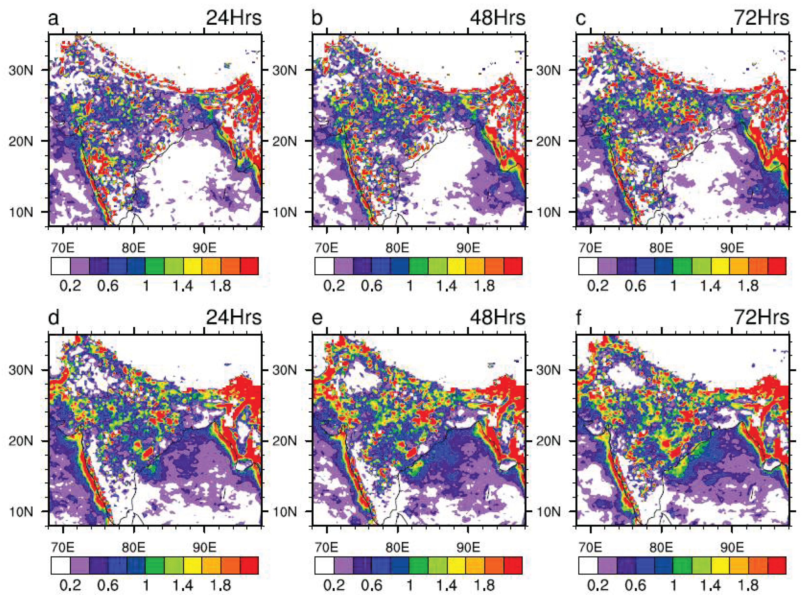
While the Probability of Detection (POD) assesses the model’s ability to correctly forecast the occurrence of extreme rainfall events, the False Alarm Rate (FAR) complements this by quantifying the frequency of incorrect or false forecasts, i.e., instances where the model predicts an event that does not occur. Together, these metrics provide a more comprehensive evaluation of forecast reliability and utility, especially in the context of high-impact events where both missed detections and false alarms carry significant consequences.
Figure 8 illustrates the spatial distribution of FAR for both GFS T1534 and MOGREPS-G at different lead times. At a 24-hour lead time, GFS T1534 exhibits relatively high FAR values across much of the Indian region, with most areas displaying FAR in the range of 0.6–0.8 (Figure 8a). This implies that a large fraction of the model’s extreme rainfall forecasts do not materialize in observations, thereby reducing the confidence in these predictions. Furthermore, the FAR values tend to increase with longer lead times, as seen in Figure 8b–c, reaching values above 0.8 in several regions by the 72-hour lead. This steady increase in FAR with forecast horizon suggests a degradation in the reliability of the GFS T1534 model in simulating extreme rainfall as the lead time extends. Furthermore analysis of FAR for MOGREPS-G, presented in Figure 8d–-f, reveals even higher values across the Indian landmass compared to GFS T1534. Despite MOGREPS-G showing relatively higher POD values at the 24-hour lead (Figure 7d), it simultaneously exhibits higher false alarm rates over majority of Indian landmass. This indicates that while the model is more successful in capturing the occurrence of extreme events, it is also more prone to over-predicting them. Interestingly, regions with higher POD values in MOGREPS-G tend to coincide with regions exhibiting higher FAR values. This spatial overlap suggests that increased detection may come at the cost of increased false alarms, raising concerns about the trade-off between sensitivity and precision in the model’s forecasts.
To evaluate the tendency of model to under/over forecast the extreme rainfall events, bias score is computed for both models and shown in Figure 9. As discussed in the methodology section a bias score of 1 implies perfect forecast while <1 (>1) implies under (over) forecast. Results obtained from GFS T1534 (Figure 9a–c) shows that model has a tendency to predominantly under-forecasts extreme rainfall events across most parts of the Indian region at all lead times. However, there are exceptions to this general behavior. The Western Ghats, Northeast India, and isolated pockets of Central India exhibit Bias Scores greater than 1.0, indicating localized over-forecasting. With increasing lead time, the model begins to exhibit over-forecasting tendencies in additional small patches across Central India, suggesting a lead-time-dependent shift in rainfall signal that could be possibly due to accumulated model errors or evolving biases in convective parameterizations.
In contrast to GFS T1534, the patches of under forecast are much less in case of MOGREPS-G over Indian region at all lead times (Figure 9d-f). MOGREPS-G displays widespread over-forecasting behaviour across the Indian landmass, with Bias Scores exceeding 1.0 in most regions even at the shortest lead time. This tendency to over-forecast becomes more pronounced as the lead time increases, indicating a systematic bias in the ensemble forecasts toward generating more extreme rainfall events than observed. These results are consistent with the previously discussed False Alarm Rate (Figure 8), where MOGREPS-G was found to have high FAR values across large parts of the country. The concurrence of high FAR and high Bias Score suggests that the over-forecasting tendency in MOGREPS-G contributes directly to the generation of numerous false alarms. Although a higher Probability of Detection (POD) was noted in MOGREPS-G at shorter lead times, the accompanying high Bias and FAR values indicate that this detection comes at the expense of forecast precision and reliability. Finally, while GFS T1534 exhibits a general tendency to under-predict extreme rainfall, MOGREPS-G shows a systematic overestimation, particularly at longer lead times. These contrasting biases underscore the need for model-specific post-processing and calibration techniques if these forecasts are to be used effectively for operational decision-making, especially in applications sensitive to both missed events and false alarms.
4. Conclusions
This study presents a comprehensive evaluation of the forecast skill of GFS T1534 and MOGREPS-G models in predicting extreme rainfall events over the Indian region during the monsoon seasons (JJAS) from 2020 to 2023. Both models generally underestimate mean seasonal rainfall and its variability, while GFS T1534 found to represent relatively better seasonal mean rainfall over the Indian landmass, MOGREPS-G performs better over the Bay of Bengal. The spatial correlation of model forecasts with observed rainfall declines with increasing lead time, more rapidly in MOGREPS-G, indicating loss of spatial coherence in forecasts beyond 24 hours. Standard deviation analysis reveals that both models fail to reproduce observed rainfall variability, a critical component for realistic simulation of extremes. GFS T1534 shows more underestimation, while MOGREPS-G occasionally overestimates variability in certain regions. To evaluate the skill of the models in predicting the extremes we fixed a uniform threshold of 50mm/day based on the values of 95th percentile rainfall. The number of R50 days were also assessed and it is found that MOGREPS-G simulates the number relatively closer to the observation over Central Indian region as compared to GFS T1534. Furthermore, POD values suggest moderate skill in detecting extreme rainfall events at short lead times, with MOGREPS-G slightly outperforming GFS T1534 at 24-hour lead. However, this advantage diminishes rapidly with longer lead times. FAR and Bias Score analyses indicate that MOGREPS-G, despite its higher detection capability, suffers from excessive over-forecasting and false alarms. GFS T1534, on the other hand, under-forecasts extremes but is somewhat relatively more conservative in its predictions. The relatively better performance of the MOGREPS-G (GFS T1534) model for day 1 (day 2 and day 3) in predicting extreme rainfall for short lead times contributes to the understanding of model performance and reliability.
Overall, while both models demonstrate potential in short-range forecasting, particularly within 24 hours, their limitations at longer lead times highlight the challenges associated with accurate prediction of extreme rainfall events. This calls for the need of further model developments and regional post-processing techniques. These insights are crucial for improving early warning systems and disaster risk reduction strategies related to extreme rainfall events in India.
Author Contributions
Conceptualization: T.G., S.R.K.; Methodology: T.G.; Formal analysis: T.G., S.R.K.; Data curation: M.G., S.R.K.; Writing original draft: T.G.; Review and editing: M.D., S.R.K., S.C. All authors have read and agreed to the published version of the manuscript.
Funding
The Indian Institute of Tropical Meteorology (Pune, India) is fully funded by the Ministry of Earth Sciences, Government of India, New Delhi. The contribution to this work by Dr. Seshagirirao Kolusu was funded by the Met Office Weather and Climate Science for Service Partnership (WCSSP) India project which is supported by the UK Department for Science, Innovation and Technology (DSIT). WCSSP India is a collaborative initiative between the Met Office and the Indian Ministry of Earth Sciences (MoES).
Data Availability Statement
The IMD-GPM data is available at IMD Pune’s website (https://imdpune.gov.in/lrfindex.php). The GFS T1534 data can be availed by requesting Director, IITM via email (director@tropmet.res.in). The MOGREPS-G data can be availed by email to Dr. Seshagirirao Kolusu (seshagirirao.kolusu@metoffice.gov.uk).
Acknowledgments
We thank IMD for providing the IMD-GPM merged data. Model runs are carried out on Mihir High Performance Computing (HPC) system at NCMRWF, New Delhi. Authors thank IITM Pratyush HPCS and NCMRWF Mihir HPCS support team for all the necessary help. Authors thank Director, IITM, Pune for motivation and encouragement in the study. The contribution to this work by SK was funded by the Met Office Weather and Climate Science for Service Partnership (WCSSP) India project which is supported by the UK Department for Science, Innovation and Technology (DSIT). WCSSP India is a collaborative initiative between the Met Office and the Indian Ministry of Earth Sciences (MoES).
Conflicts of Interest
The author SC is the Guest Editor of a Special Issue, Novel Approaches to Predict Extreme Events in Atmospheric Flows: From Turbulence to Climate.
References
- Gordon, H.; Whetton, P.; Pittock, A.; Fowler, A.; Haylock, M. Simulated changes in daily rainfall intensity due to the enhanced greenhouse effect: Implications for extreme rainfall events. Climate Dynamics 1992, 8, 83–102. [Google Scholar] [CrossRef]
- Hennessy, K.; Gregory, J.M.; Mitchell, J. Changes in daily precipitation under enhanced greenhouse conditions. Climate Dynamics 1997, 13, 667–680. [Google Scholar] [CrossRef]
- Easterling, D.R.; Evans, J.L.; Groisman, P.Y.; Karl, T.R.; Kunkel, K.E.; Ambenje, P. Observed variability and trends in extreme climate events: A brief review. Bulletin of the American Meteorological Society 2000, 81, 417–426. [Google Scholar] [CrossRef]
- Trenberth, K.E.; Dai, A.; Rasmussen, R.M.; Parsons, D.B. The changing character of precipitation. Bulletin of the American Meteorological Society 2003, 84, 1205–1218. [Google Scholar] [CrossRef]
- Min, S.K.; Zhang, X.; Zwiers, F.W.; Hegerl, G.C. Human contribution to more-intense precipitation extremes. Nature 2011, 470, 378–381. [Google Scholar] [CrossRef] [PubMed]
- Allan, R.P.; Soden, B.J.; John, V.O.; Ingram, W.; Good, P. Current changes in tropical precipitation. Environmental Research Letters 2010, 5, 025205. [Google Scholar] [CrossRef]
- Wernberg, T.; Smale, D.A.; Tuya, F.; Thomsen, M.S.; Langlois, T.J.; De Bettignies, T.; Bennett, S.; Rousseaux, C.S. An extreme climatic event alters marine ecosystem structure in a global biodiversity hotspot. Nature Climate Change 2013, 3, 78–82. [Google Scholar] [CrossRef]
- Curtis, S.; Fair, A.; Wistow, J.; Val, D.V.; Oven, K. Impact of extreme weather events and climate change for health and social care systems. Environmental Health 2017, 16, 128. [Google Scholar] [CrossRef] [PubMed]
- Liang, S.; Wang, D.; Ziegler, A.D.; Li, L.Z.; Zeng, Z. Madden–Julian Oscillation-induced extreme rainfalls constrained by global warming mitigation. npj Climate and Atmospheric Science 2022, 5, 67. [Google Scholar] [CrossRef]
- Goswami, B.N.; Venugopal, V.; Sengupta, D.; Madhusoodanan, M.; Xavier, P.K. Increasing trend of extreme rain events over India in a warming environment. Science 2006, 314, 1442–1445. [Google Scholar] [CrossRef]
- Rajeevan, M.; Bhate, J.; Jaswal, A.K. Analysis of variability and trends of extreme rainfall events over India using 104 years of gridded daily rainfall data. Geophysical research letters 2008, 35. [Google Scholar]
- Ajayamohan, R.; Merryfield, W.J.; Kharin, V.V. Increasing trend of synoptic activity and its relationship with extreme rain events over central India. Journal of Climate 2010, 23, 1004–1013. [Google Scholar] [CrossRef]
- Pattanaik, D.; Rajeevan, M. Variability of extreme rainfall events over India during southwest monsoon season. Meteorological Applications 2010, 17, 88–104. [Google Scholar] [CrossRef]
- Pal, L.; Ojha, C.S.P.; Dimri, A. Characterizing rainfall occurrence in India: Natural variability and recent trends. Journal of Hydrology 2021, 603, 126979. [Google Scholar] [CrossRef]
- Singh, D.; Tsiang, M.; Rajaratnam, B.; Diffenbaugh, N.S. Observed changes in extreme wet and dry spells during the South Asian summer monsoon season. Nature Climate Change 2014, 4, 456–461. [Google Scholar] [CrossRef]
- Roxy, M.K.; Ghosh, S.; Pathak, A.; Athulya, R.; Mujumdar, M.; Murtugudde, R.; Terray, P.; Rajeevan, M. A threefold rise in widespread extreme rain events over central India. Nature communications 2017, 8, 708. [Google Scholar] [CrossRef]
- Durman, C.; Gregory, J.M.; Hassell, D.C.; Jones, R.; Murphy, J. A comparison of extreme European daily precipitation simulated by a global and a regional climate model for present and future climates. Quarterly Journal of the Royal Meteorological Society 2001, 127, 1005–1015. [Google Scholar] [CrossRef]
- Li, F.; Collins, W.D.; Wehner, M.F.; Williamson, D.L.; Olson, J.G. Response of precipitation extremes to idealized global warming in an aqua-planet climate model: Towards a robust projection across different horizontal resolutions. Tellus A: Dynamic Meteorology and Oceanography 2011, 63, 876–883. [Google Scholar] [CrossRef]
- Mukhopadhyay, P.; Prasad, V.; Krishna, R.P.M.; Deshpande, M.; Ganai, M.; Tirkey, S.; Sarkar, S.; Goswami, T.; Johny, C.; Roy, K.; et al. Performance of a very high-resolution global forecast system model (GFS T1534) at 12.5 km over the Indian region during the 2016–2017 monsoon seasons. Journal of Earth System Science 2019, 128, 155. [Google Scholar] [CrossRef]
- Arora, K.; Ashrit, R.; Iyengar, G.; Rajagopal, E. MOGREPS Temperatures and Total Precipitation Climatology Over India. Technical report, NCMRWF, 2016.
- Sela, J.G. The derivation of the sigma pressure hybrid coordinate semi-Lagrangian model equations for the GFS. Technical report, NOAA, 2010.
- Han, J.; Pan, H.L. Revision of convection and vertical diffusion schemes in the NCEP Global Forecast System. Weather and Forecasting 2011, 26, 520–533. [Google Scholar] [CrossRef]
- Zhao, Q.; Carr, F.H. A prognostic cloud scheme for operational NWP models. Monthly Weather Review 1997, 125, 1931–1953. [Google Scholar] [CrossRef]
- Prasad, V.; Johny, C.; Sodhi, J.S. Impact of 3D Var GSI-ENKF hybrid data assimilation system. Journal of Earth System Science 2016, 125, 1509–1521. [Google Scholar] [CrossRef]
- Bowler, N.E.; Arribas, A.; Mylne, K.R.; Robertson, K.B.; Beare, S.E. The MOGREPS short-range ensemble prediction system. Quarterly Journal of the Royal Meteorological Society 2008, 134, 703–722. [Google Scholar] [CrossRef]
- Gregory, D.; Kershaw, R.; Inness, P. Parametrization of momentum transport by convection. II: Tests in single-column and general circulation models. Quarterly Journal of the Royal Meteorological Society 1997, 123, 1153–1183. [Google Scholar] [CrossRef]
- Wilson, D.R.; Ballard, S.P. A microphysically based precipitation scheme for the UK Meteorological Office Unified Model. Quarterly Journal of the Royal Meteorological Society 1999, 125, 1607–1636. [Google Scholar] [CrossRef]
- Walters, D.; Baran, A.J.; Boutle, I.; Brooks, M.; Earnshaw, P.; Edwards, J.; Furtado, K.; Hill, P.; Lock, A.; Manners, J.; et al. The Met Office Unified Model global atmosphere 7.0/7.1 and JULES global land 7.0 configurations. Geoscientific Model Development 2019, 12, 1909–1963. [Google Scholar] [CrossRef]
- Mitra, A.K.; Prakash, S.; Pai, D. Operational 24-hour accumulated rainfall dataset over Indian region by merging rain gauge and multi-satellite estimate from ‘Global Precipitation Measurement’mission. Journal of Earth System Science 2025, 134, 1–12. [Google Scholar] [CrossRef]
- Wilks, D.S. Statistical methods in the atmospheric sciences; Vol. 100, Academic press, 2011.
Figure 1.
Spatial pattern of mean JJAS rainfall (mm/day) from (a) IMD-GPM, (b–d) GFS T1534, (e–g) MOGREPS-G. (b,e), (c,f) and (d,g) represents 24hr, 48hr and 72hr forecast respectively.
Figure 1.
Spatial pattern of mean JJAS rainfall (mm/day) from (a) IMD-GPM, (b–d) GFS T1534, (e–g) MOGREPS-G. (b,e), (c,f) and (d,g) represents 24hr, 48hr and 72hr forecast respectively.
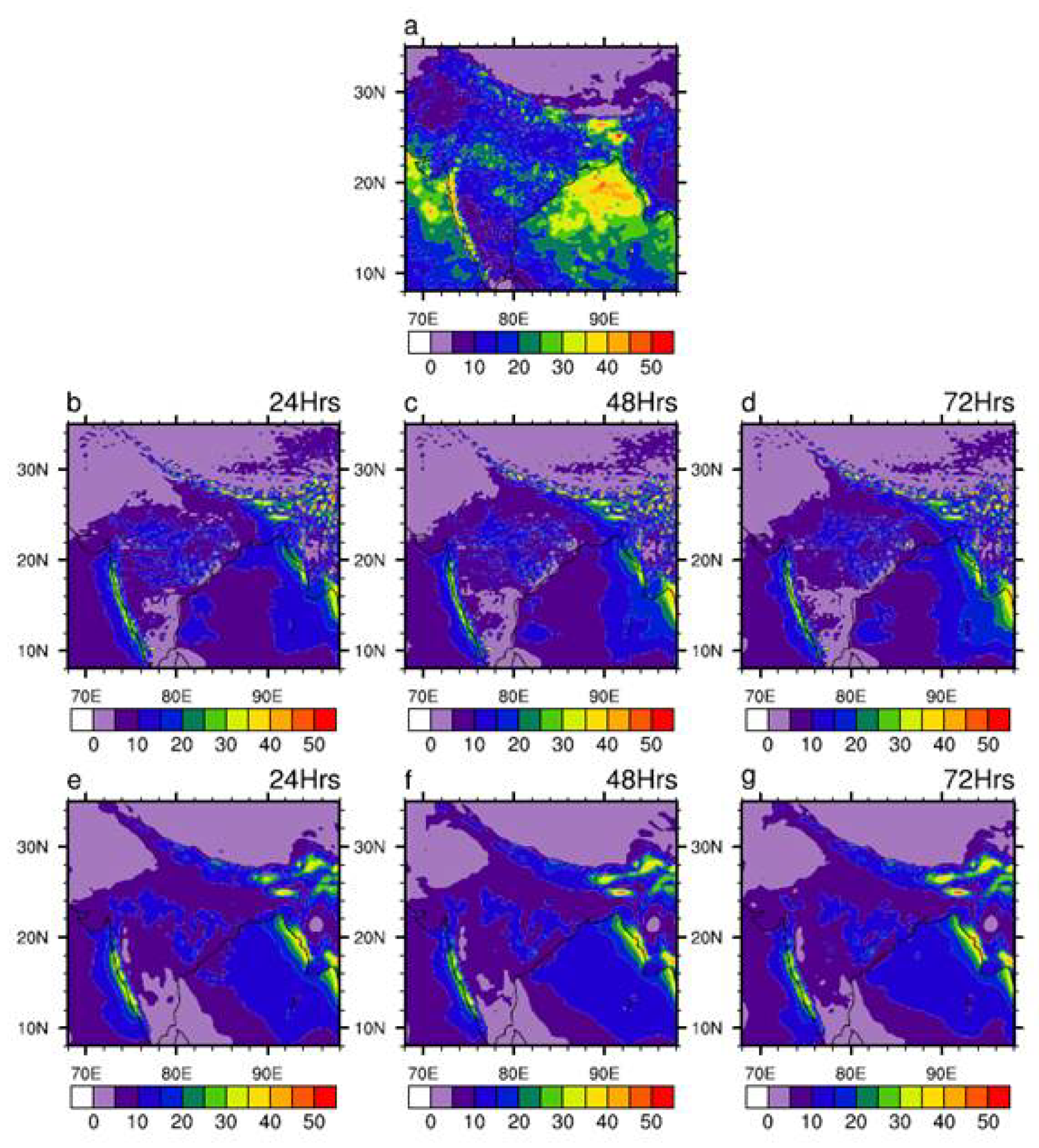
Figure 2.
Spatial pattern of correlation between observation and models. (a-c) GFS T1534 and (d-f) MOGREPS-G. First, second and third column represents 24hr, 48hr and 72hr forecast respectively.
Figure 2.
Spatial pattern of correlation between observation and models. (a-c) GFS T1534 and (d-f) MOGREPS-G. First, second and third column represents 24hr, 48hr and 72hr forecast respectively.
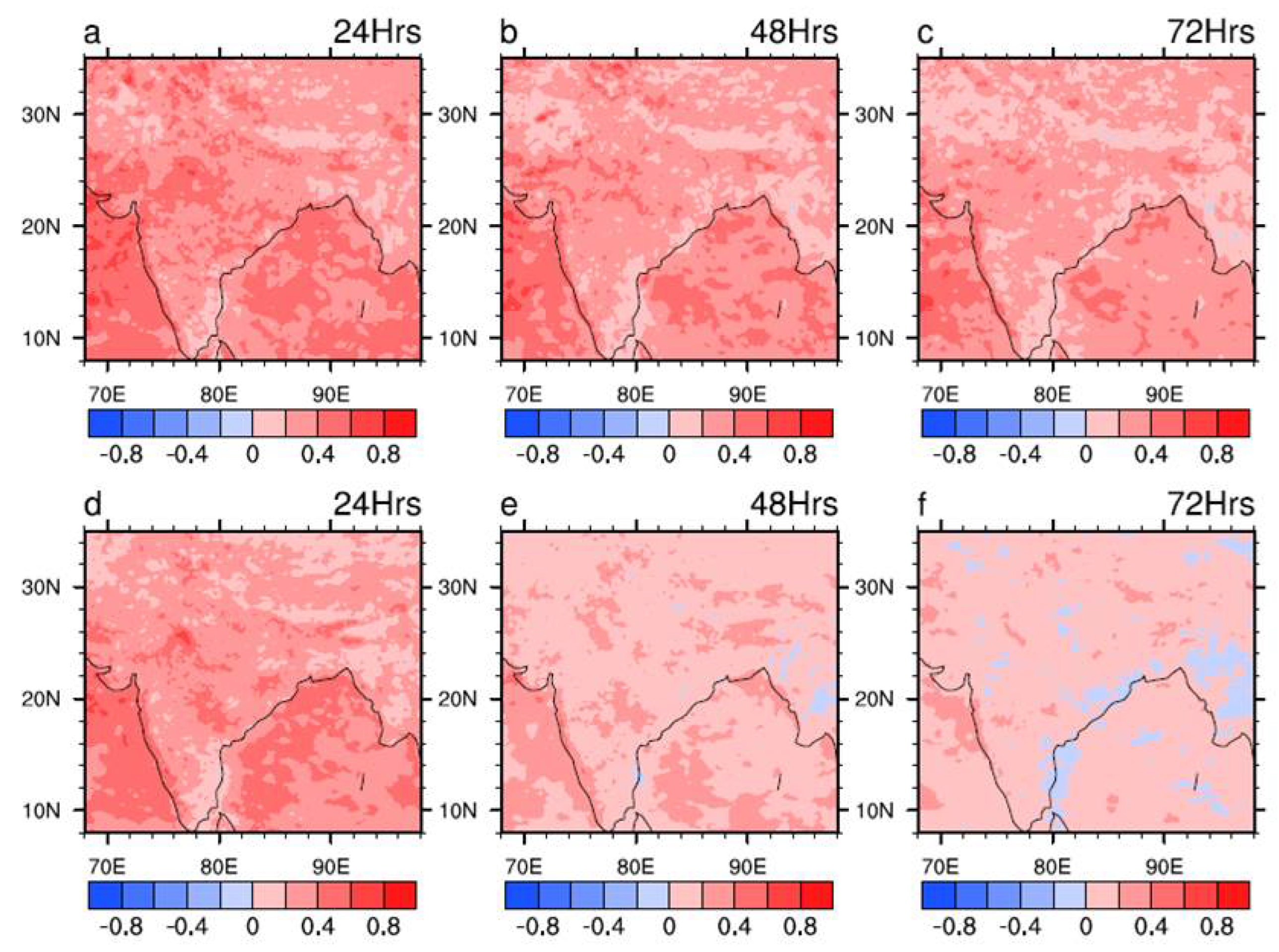
Figure 3.
Spatial pattern of standard deviation (mm/day) of JJAS rainfall derived from (a) IMD-GPM, (b-d) GFS T1534, (e–g) MOGREPS-G. (b,e), (c,f) and (d,g) represents 24hr, 48hr and 72hr forecast respectively.
Figure 3.
Spatial pattern of standard deviation (mm/day) of JJAS rainfall derived from (a) IMD-GPM, (b-d) GFS T1534, (e–g) MOGREPS-G. (b,e), (c,f) and (d,g) represents 24hr, 48hr and 72hr forecast respectively.
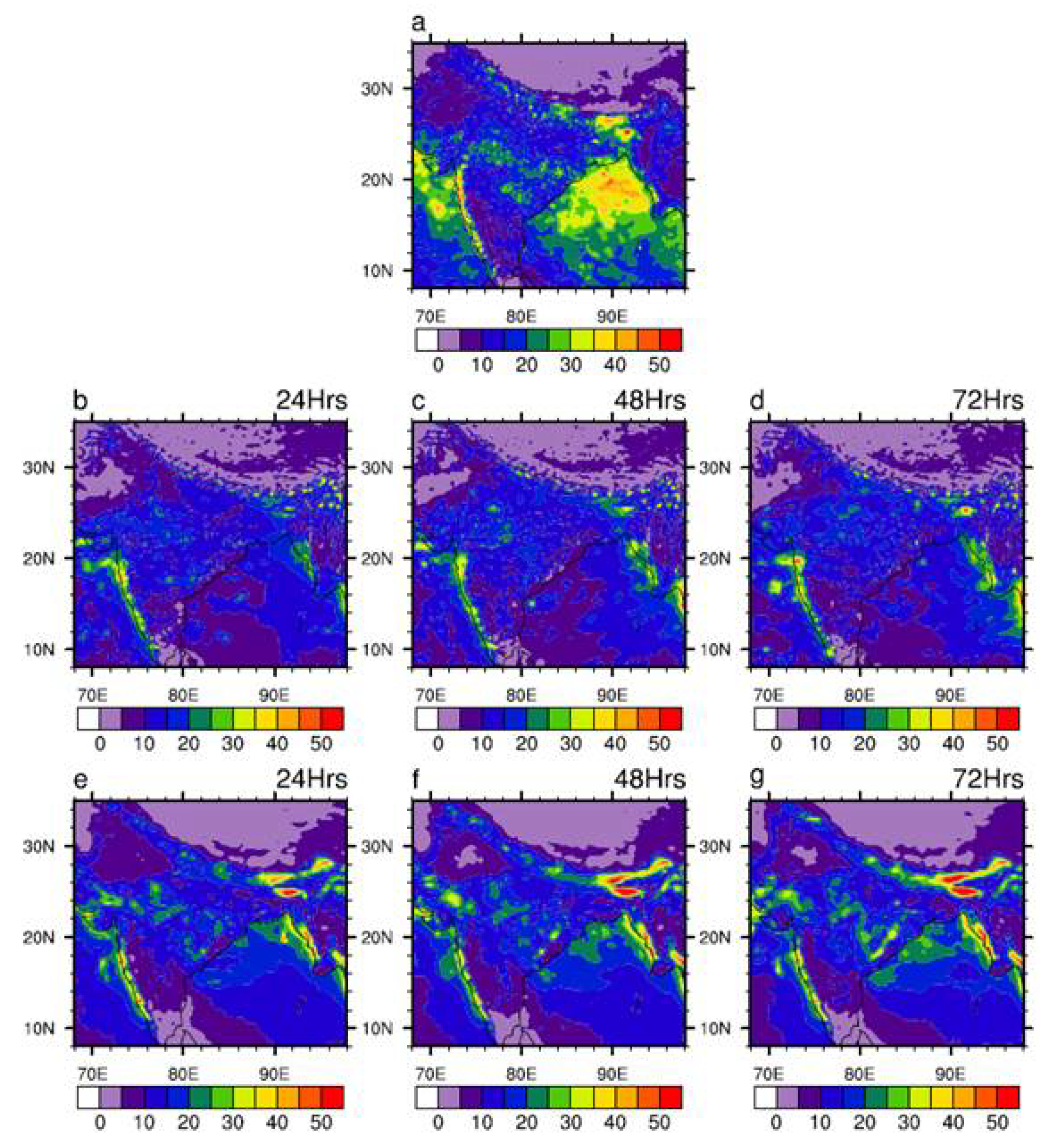
Figure 4.
Spatial pattern of 95th percentile threshold (mm/day) of JJAS rainfall derived from (a) IMD-GPM, (b-d) GFS T1534, (e–g) MOGREPS-G. (b,e), (c,f) and (d,g) represents 24hr, 48hr and 72hr forecast respectively.
Figure 4.
Spatial pattern of 95th percentile threshold (mm/day) of JJAS rainfall derived from (a) IMD-GPM, (b-d) GFS T1534, (e–g) MOGREPS-G. (b,e), (c,f) and (d,g) represents 24hr, 48hr and 72hr forecast respectively.
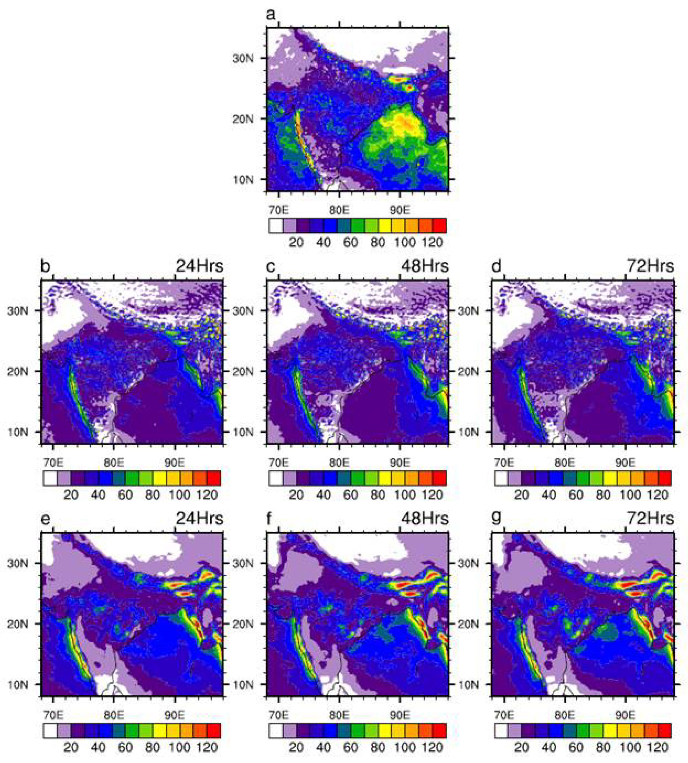
Figure 5.
Spatial pattern of R50 days during JJAS derived from (a) IMD-GPM, (b–d) GFS T1534, (e–g) MOGREPS-G. (b,e), (c,f) and (d,g) represents 24hr, 48hr and 72hr forecast respectively.
Figure 5.
Spatial pattern of R50 days during JJAS derived from (a) IMD-GPM, (b–d) GFS T1534, (e–g) MOGREPS-G. (b,e), (c,f) and (d,g) represents 24hr, 48hr and 72hr forecast respectively.
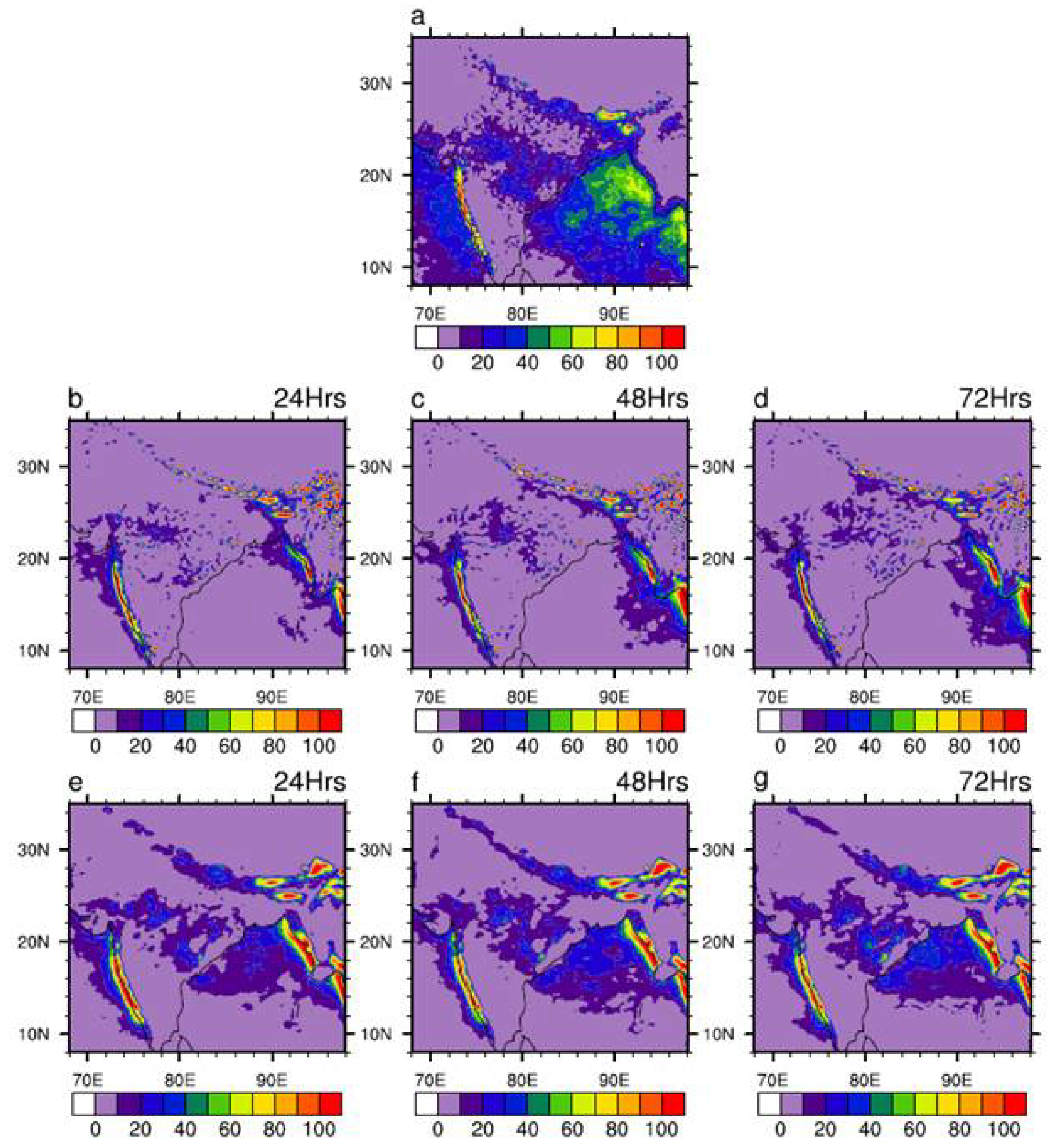
Figure 6.
Spatial pattern of R150 days during JJAS derived from (a) IMD-GPM, (b–d) GFS T1534, (e–g) MOGREPS-G. (b,e), (c,f) and (d,g) represents 24hr, 48hr and 72hr forecast respectively.
Figure 6.
Spatial pattern of R150 days during JJAS derived from (a) IMD-GPM, (b–d) GFS T1534, (e–g) MOGREPS-G. (b,e), (c,f) and (d,g) represents 24hr, 48hr and 72hr forecast respectively.
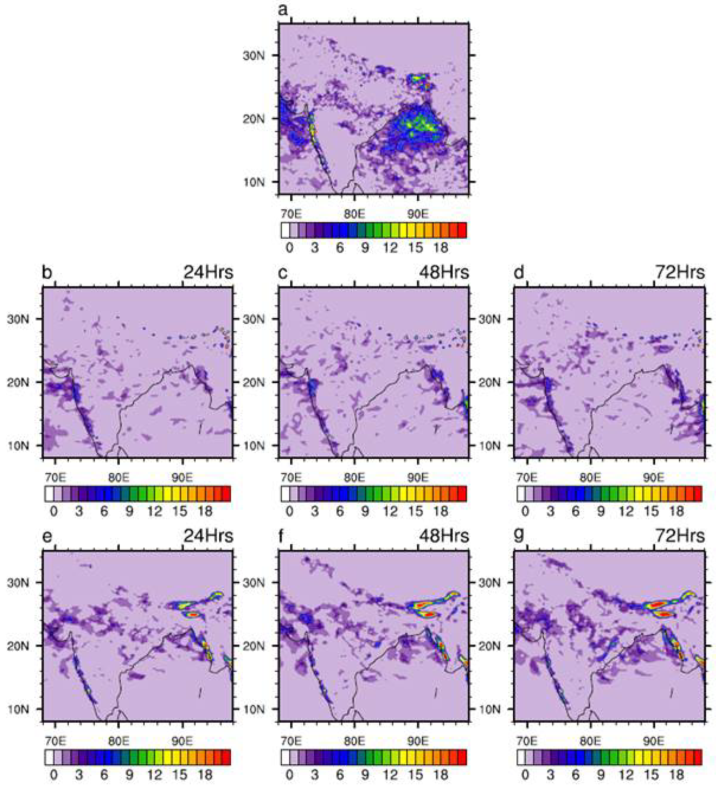
Figure 7.
Spatial distribution of Probability of Detection (POD) for rainfall over 50 mm/day obtained from (a–c) GFS T1534 and (d–f) MOGREPS-G. First, second and third column represents 24hr, 48hr and 72hr forecast respectively.
Figure 7.
Spatial distribution of Probability of Detection (POD) for rainfall over 50 mm/day obtained from (a–c) GFS T1534 and (d–f) MOGREPS-G. First, second and third column represents 24hr, 48hr and 72hr forecast respectively.
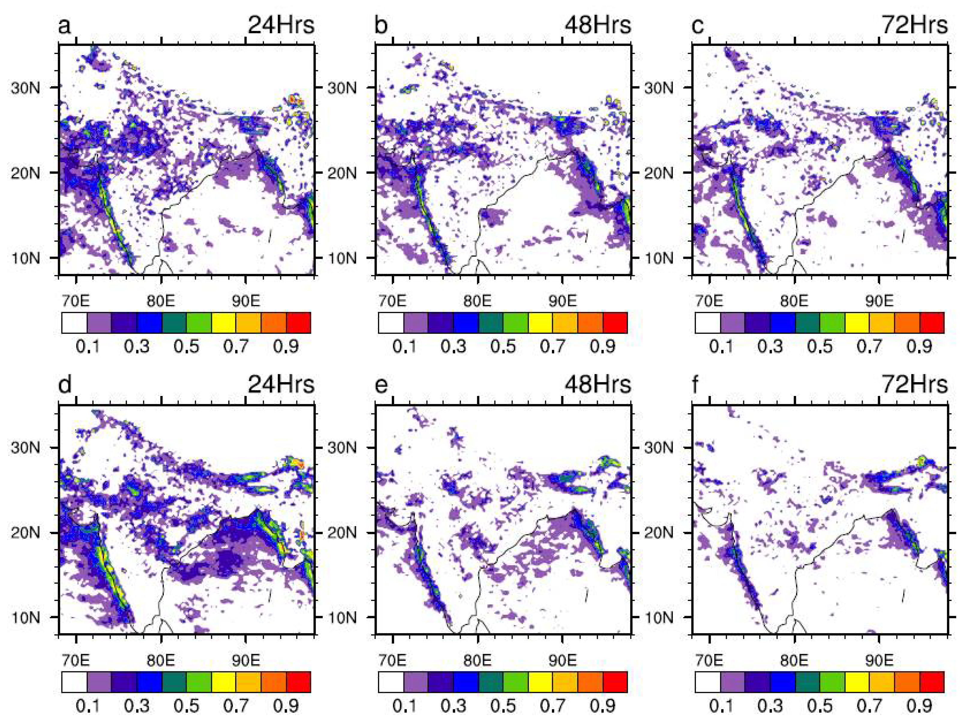
Figure 8.
Spatial distribution of False Alarm Rate (FAR) for rainfall over 50 mm/day obtained from (a-c) GFS T1534 and (d-f) MOGREPS-G. First, second and third column represents 24hr, 48hr and 72hr forecast respectively.
Figure 8.
Spatial distribution of False Alarm Rate (FAR) for rainfall over 50 mm/day obtained from (a-c) GFS T1534 and (d-f) MOGREPS-G. First, second and third column represents 24hr, 48hr and 72hr forecast respectively.
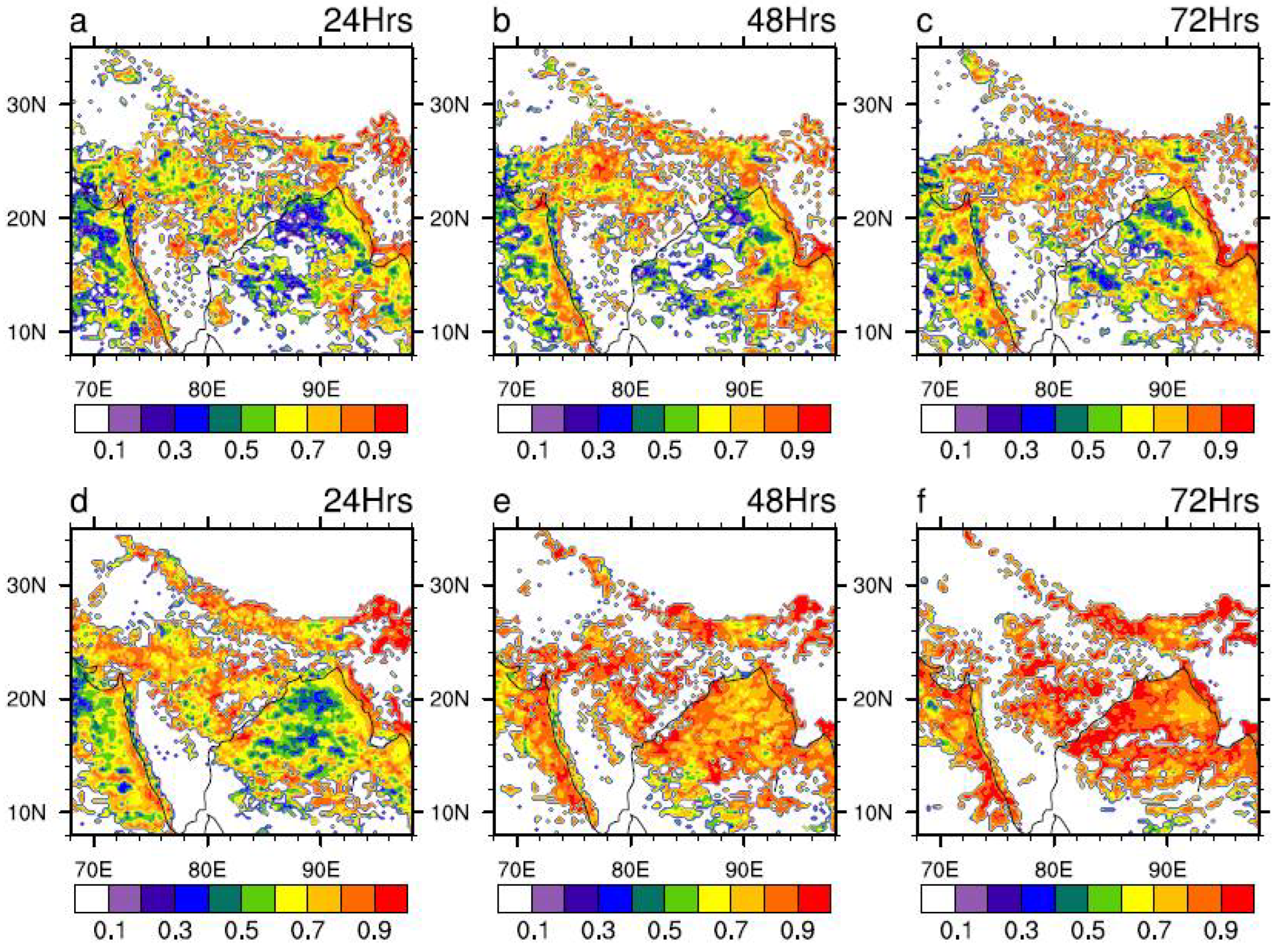
Figure 9.
Spatial distribution of forecast Bias for rainfall over 50 mm/day computed from equation 3 for (a-c) GFS T1534 and (d-f) MOGREPS-G. First, second and third column represents 24hr, 48hr and 72hr forecast respectively.
Figure 9.
Spatial distribution of forecast Bias for rainfall over 50 mm/day computed from equation 3 for (a-c) GFS T1534 and (d-f) MOGREPS-G. First, second and third column represents 24hr, 48hr and 72hr forecast respectively.
Disclaimer/Publisher’s Note: The statements, opinions and data contained in all publications are solely those of the individual author(s) and contributor(s) and not of MDPI and/or the editor(s). MDPI and/or the editor(s) disclaim responsibility for any injury to people or property resulting from any ideas, methods, instructions or products referred to in the content. |
© 2025 by the authors. Licensee MDPI, Basel, Switzerland. This article is an open access article distributed under the terms and conditions of the Creative Commons Attribution (CC BY) license (http://creativecommons.org/licenses/by/4.0/).
Copyright: This open access article is published under a Creative Commons CC BY 4.0 license, which permit the free download, distribution, and reuse, provided that the author and preprint are cited in any reuse.


