
Submitted:
26 July 2025
Posted:
28 July 2025
You are already at the latest version
Abstract
This work addresses the mathematical modeling of the Inverse Problem in cardiac electrophysiology. The Forward Problem aims to compute the potential field on the body surface generated by electrical sources within the heart, while the Inverse Problem seeks to reconstruct these internal sources based on body surface measurements. This research focuses on solving the Inverse Problem by formulating it in terms of transmembrance potentials (TMPs) rather than current density vectors, which significantly reduces the solution domain and computational cost. Three modeling scenarios are explored: an isotropic volume source in an infinite homogeneous volume conductor, an anisotropic source in a homogeneous medium, and an anisotropic source in an inhomogeneous medium. Each scenario leads to a different lead field transfer matrix formulation, ultimately enabling the reconstruction of cardiac TMPs from body surface potential maps (BSPMs). The linearity of the resulting system validates the application of advanced linear regularization methods.
Keywords:
Cardiac electrophysiology
; Inverse problem
; Transmembrance potential (TMP)
; Body surface potential map (BSPM)
1. Introduction
There are two problems in modeling the electrophysiology of the heart: the Forward Problem and the Inverse Problem [1]. The heart Forward Problem involves designing a model that is capable of determining the field on the surface of known body (conductor) that is generated by electrical-sources inside the heart. Solving the Forward Problem requires the development of electrical models which are capable of describing the bioelectrical criteria of the heart and the body (Figure 1).
Formulating the Inverse Problem requires identifying the configuration of the volume source. The heart can be considered as one dipole source that generate the field as introduced in [2,3,4], where in Cartesian coordinates, six parameters are required to identify that source; three for location and three for direction. One of the most used source models is the potential distribution on the Epicardium surface from the body surface reading as described in [5,6,7,8,9,10,11,12,13,14,15,16,17,18,19]. This will provide an indication about the source distribution inside the heart. Finally, the most recent models use the multiple pole source distribution, where it is required to identify the distribution of electrical sources in the heart volume directly [20,21,22,23,24,25,26,27]. Instead of formulating the Inverse Problem in terms of current densities distributions as demonstrated in other research, the formulation of the problem in this research will be in terms of transmembrance potentials.
Formulating the problem in terms of TMP reduces the solution domain size to the 1/3 of the current density solutions, as each location inside the heart will be represented as one variable instead of the three variables for each component of the current density vector. Some operations (matrix multiplication and matrix inversion) of the Inverse Problem solutions are of cubic complexity, O(N3), and so reducing the solution domain size will decrease the computation cost.
Moreover, reducing the solution domain size will reduce the ‘underdeterminity’ of the system since providing fewer unknowns (independent variables) to the regularization process with the same number of results (dependent variables) will lead to a better solution.
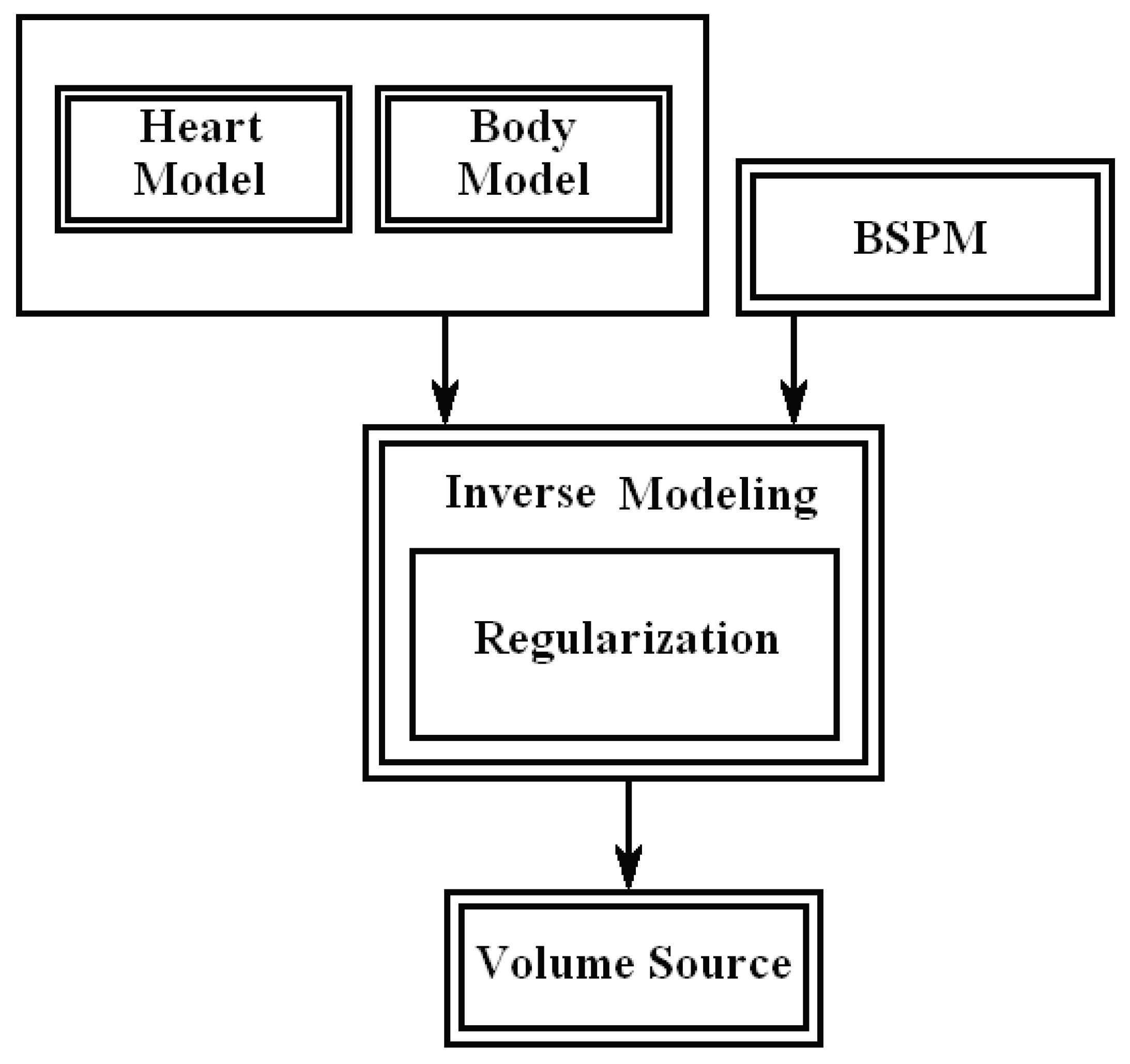
The stages of the Inverse Problem solution are performed as shown in Figure 2, where the heart model [28,29,30,31,32,33,34] and the body model [35] are used to build the lead field transfer matrix and the BSPM (the output of the Forward Model solution) [36] is used as the dependent variables vector.
The main objective here is to build a transfer matrix A that maps the transmembrance potentials x to the body surface potential b such that
where A is MxN transfer matrix, b is Mx1 body surface reading vector, and x is Nx1 TMP vector.
Formulation of the Inverse Problem is introduced for both homogeneous and inhomogeneous volume conductor and the volume source conductivity-tensor can be either isotropic or anisotropic, leading to different lead field transfer matrices. Three settings are introduced in this research, isotropic volume source in infinite homogeneous volume conductor, anisotropic volume source in infinite homogeneous volume conductor and anisotropic volume source in inhomogeneous volume conductor. The first is the simplest setting which requires the least information about the volume source and the volume conductor, but it is also the most inaccurate model among the three models.
2. Transfer Matrix of Isotropic Volume Source in Infinite Homogeneous Volume Conductor
Consider the equation of calculating the potential in an infinite homogenous volume conductor:
where σ0 is the homogeneous volume conductor conductivity, σi is the volume source conductivity tensor, Vm is the transmembrance potential, and r is the observation point to source point vector.
By assuming isotropic conductivity-tensor of the source and equal to the conductivity of the volume source medium then equation (2) can be written as
and then
where N is the number of sources and δv is a unit volume. The gradient of transmembrance potential and the vector r can be written in Cartesian coordinates as
then
using Taylor’s theorem
Then in the X direction, the current element will contribute by to the next element and by to the previous element, and so on for Y and Z directions.
Finally, each element in the transfer matrix A can be built as
where these elements represents the six orthogonal neighbors of the current node with respect to an observation point in the Cartesian coordinate system. Then, for M body-surface locations, the forward solution of the infinite homogeneous volume conductor can be written as
where b0 is the vector of the dependent variables, x is the vector of the independent variables, and A0 is the lead field transfer matrix.
3. Transfer Matrix of Anisotropic Volume Source in Infinite Homogeneous Volume Conductor
The approach is taken as the previous section, but the conductivity tensor of the source is considered here to be anisotropic. Due to orthogonality of the conductivity tensor, the calculations can be in terms of the principal direction (first eigenvector) of the tensor. Equation (11) shows the equation in terms of principal direction e as
where e is the tensor’s principal direction vector, eT is the transpose of this vector, and σl and σt is the longitudinal and traverse conductivities, respectively. The term can be written in the X coordinate as
Finally, each element in the transfer matrix A(i,j) can be built as
and the forward solution will be the same as equation (10)
4. Transfer Matrix of a Volume Source in Inhomogeneous Volume Conductor
The equation that calculates the potential field at any point inside an inhomogeneous volume conductor is defined as [Ref_102]:
where is the potential of the infinite homogeneous volume conductor (eq. 2), k is the organ’s number, L is the number of organs, Sk is the surface of the organ, and are the conductivities just inside and just outside the organ’s boundary, is the equation (2), is the displacement vector from primary source to a point on the organ boundary, is the displacement vector from boundary surface (secondary source) to body surface and is the normal vector on the organ’s boundary surface and it points to the outside of the organ. Then, for an observation point W, and can be written as in equation (10) as the following
such that AkT represents the row of elements (a vector transpose) belonging to the observation point W in the matrix A of the organ k. For any point W on the body surface, equation (14) can be written as
where Pk denotes the number of surfaces in the organ k, δS is a surface element area, r is the vector from an observation point W to a point on the surface of an organ k, and n is the normal vector at this point. Then for each organ, the partial transfer matrix will be
Building the partial transfer matrix using equation (17) can be performed as follows
- 1-
- Compute the transfer matrix A of the organ or the body torso to all sources inside the heart using Equation 13. (Equation 9 can be used also in case of no information about fibers directions).
- 2-
- Tessellate the organ’s surface into triangular elements and calculate the normal vectors on each surface element done by cross product of any two edges of the triangle in anti-clock-wise direction and calculate the area of the triangle element can be derived from the dot product of two these edges.
- 3-
- From each point on the body surface, compute the vector r to a point on an organ surface element.
- 4-
- Compute the scalar
- 5-
- Multiply the last scalar by the corresponding row (the row of the current observation point) in the corresponding A matrix, and add this row in a new matrix .
When applying these steps to all organs, Equation 16 becomes
which can be written as
or in the form of equation (1)
5. Conclusions
This research develops a comprehensive framework for modeling and solving the cardiac Inverse Problem using transmembrance potentials. By reformulating the problem in terms of TMPs instead of current densities, the solution space is reduced by two-thirds, resulting in significant computational efficiency and improved system conditioning. The study derives and constructs lead field transfer matrices under three increasingly complex biophysical conditions: isotropic-homogeneous, anisotropic-homogeneous, and anisotropic-inhomogeneous conductors. The final formulation maintains linearity, ensuring compatibility with established linear regularization techniques such as MN, WMN, and LORETA. This approach provides a robust foundation for accurate non-invasive cardiac source imaging, potentially enhancing clinical diagnosis and treatment planning in electrophysiology.
References
- Malmivuo, J.; Plonsey, R. Bioelectromagnetism: Principles and Applications of Bioelectric and Biomagnetic Fields, 1st ed.; Oxford Univ. Press, 1995; ISBN 0195058232. [Google Scholar]
- Nenonen, J.; Purell, C.J.; Horacek, B.M.; Stroink, G.; Katila, T. Magnetocardiographic functional localization using a current dipole in a realistic torso. IEEE Trans. Biomed. Eng. 1991, 38, 658–664. [Google Scholar] [CrossRef]
- Purcell, C.J.; Stroink, G. Moving dipole inverse solutions using realistic torso models. IEEE Trans. Biomed. Eng. 1991, 38, 82–84. [Google Scholar] [CrossRef]
- Tan, G.A.; Brauer, F.; Stroink, G.; Purcell, C.J. The effect of measurement conditions on MCG inverse solutions. IEEE Trans. Biomed. Eng. 1992, 39, 921–927. [Google Scholar] [CrossRef]
- Seger, M. Modeling the Electrical Function of the Human Heart. Ph.D. Thesis, Institute of Biomedical Engineering, University for Health Sciences, Medical Informatics and Technology, Austria, 2006. [Google Scholar]
- Brooks, D.H.; MacLeody, R.S. Electrical Imaging of the Heart: Electrophysical Underpinnings and Signal Processing Opportunities. IEEE Signal Processing 1996, 14, 24–42. [Google Scholar] [CrossRef]
- Hintermuller, C. Development of a Multi-Lead ECG Array for Noninvasive Imaging of the Cardiac Electrophysiology. Ph.D. Thesis, Institute of Biomedical Engineering, University for Health Sciences, Medical Informatics and Technology, Austria, 2006. [Google Scholar]
- Messinger-Rapport, B.J.; Rudy, Y. Noninvasive recovery of epicardial potentials in a realistic heart- torso geometry. Normal sinus rhythm. American Heart Association 1990, 66, 1023–1039. [Google Scholar]
- Oster, H.S.; Taccardi, B.; Lux, R.L.; Ershler, P.R.; Rudy, Y. Electrocardiographic Imaging : Noninvasive Characterization of Intramural Myocardial Activation From Inverse-Reconstructed Epicardial Potentials and Electrograms. American Heart Association 1998, 97, 1496–1507. [Google Scholar] [CrossRef]
- Berger, T.; Fischer, G.; Pfeifer, B.; Modre, R.; Hanser, F.; Roithinger, F.X.; Stuehlinger, M.; Pachinger, O.; Hintringer, F. Single-Beat Noninvasive Imaging of Cardiac Electrophysiology of Ventricular Pre-Excitation. J. Am. Coll. Cardiol. 2006, 48, 2045–2052. [Google Scholar] [CrossRef]
- Cheng, L. Non-Invasive Electrical Imaging of the Heart. Ph.D. Thesis, The University of Auckland, New Zealand, 2001. [Google Scholar]
- Ramanathan, C.; Jia, P.; Ghanem, R.; Calvetti, D.; Rudy, Y. Noninvasive Electrocardiographic Imaging (ECGI):Application of the Generalized Minimal Residual (GMRes) Method. Ann. Biomed. Eng. 2003, 31, 981–994. [Google Scholar] [CrossRef] [PubMed]
- Ghanem, R.N.; Ramanathan, C.; Ryu, K.; Markowitz, A.; Rudy, Y. Noninvasive Electrocardiographic Imaging (ECGI): Comparison to intraoperative mapping in patients. Heart Rhythm. 2005, 2, 339–354. [Google Scholar] [CrossRef] [PubMed]
- Intini, R.; Goldstein, R.; Jia, P.; Ramanathan, C.; Stambler, B.S.; Rudy, Y.; Waldo, A.L. A novel diagnostic modality used for mapping of focal left ventricular tachycardia in a young athlete. Heart Rhythm. 2005, 2, 1250–1252. [Google Scholar] [CrossRef]
- Jia, P.; Rudy, Y. Electrocardiographic imaging of cardiac resynchronization therapy in heart failure: Observation of variable electrophysiologic responses. Heart Rhythm. 2006, 3, 296–310. [Google Scholar] [CrossRef]
- Ghanem, R.N.; Ramanathan, C.; Jia, P.; Rudy, Y. Heart-Surface Reconstruction and ECG Electrodes Localization Using Fluoroscopy, Epipolar Geometry and Stereovision:Application to Noninvasive Imaging of Cardiac Electrical Activity. IEEE Trans. Med. Imaging. 2003, 22, 1307–1318. [Google Scholar] [CrossRef]
- Berger, T.; Hintringer, F.; Fischer, G. Noninvasive Imaging of Cardiac Electrophysiology. Indian Pacing and Electrophysiology Journal 2007, 7, 160–165. [Google Scholar]
- Ramanathan, C.; Ghanem, R.N.; Jia, P.; Ryu, K.; Rudy, Y. Noninvasive electrocardiographic imaging for cardiac electrophysiology and arrhythmia. Nat Med. 2004, 10, 422–428. [Google Scholar] [CrossRef]
- Ghosh, S.; Rudy, Y. Accuracy of Quadratic Versus Linear Interpolation in Noninvasive Electrocardiographic Imaging (ECGI). Ann. Biomed. Eng. 2005, 33, 1187–1201. [Google Scholar] [CrossRef] [PubMed]
- Seger, M.; Modre, R.; Pfeifer, B.; Hintermuller, C.; Tilg, B. Non-invasive Imaging of Atrial Flutter. Computers in Cardiology 2006, 33, 601–604. [Google Scholar]
- Zhang, X.; Ramachandra, I.; Liu, Z.; Muneer, B.; Pogwizd, S.M.; He, B. Noninvasive three-dimensional electrocardiographic imaging of ventricular activation sequence. Am J Physiol Heart Circ Physiol 2005, 289, H2724–H2732. [Google Scholar] [CrossRef] [PubMed]
- Xanthis, C.G.; Bonovas, P.M.; Kyriacou, G.A. Inverse Problem of ECG for Direrent Equivalent Cardiac Sources. PIERS Online 2007, 3, 1222–1227. [Google Scholar] [CrossRef]
- He, B.; Li, G.; Zhang, X. Noninvasive Imaging of Cardiac Transmembrane Potentials Within Three-Dimensional Myocardium by Means of a Realistic Geometry Anisotropic Heart Model. IEEE Trans. Biomed. Eng. 2003, 50, 1190–1202. [Google Scholar]
- He, B.; Wu, D. Imaging and Visualization of 3-D Cardiac Electric Activity. IEEE Tran. Inf Tech. Biomed. 2001, 5, 181–186. [Google Scholar]
- Li, G.; Zhang, X.; Lian, J.; He, B. Noninvasive Localization of the Site of Origin of Paced Cardiac Activation in Human by Means of a 3-D Heart Model. IEEE Trans. Biomed. Eng. 2003, 50, 1117–1120. [Google Scholar]
- Liu, Z.; Liu, C.; He, B. Noninvasive Reconstruction of Three-Dimensional Ventricular Activation Sequence From the Inverse Solution of Distributed Equivalent Current Density. IEEE Trans. Med. Imag. 2006, 25, 1307–1318. [Google Scholar]
- He, B.; Liu, C.; Zhang, Y. Three-Dimensional Cardiac Electrical Imaging From Intracavity Recordings. IEEE Trans. Biomed. Eng. 2007, 54, 1454–1460. [Google Scholar] [CrossRef] [PubMed]
- Elaff, I. Modeling of realistic heart electrical excitation based on DTI scans and modified reaction diffusion equation. Turkish Journal of Electrical Engineering and Computer Sciences 2018, 26, 2. [Google Scholar] [CrossRef]
- El-Aff, I.A.I. Extraction of human heart conduction network from diffusion tensor MRI. The 7th IASTED International Conference on Biomedical Engineering, 217–222.
- Elaff, I. Modeling of the Human Heart in 3D Using DTI Images. World Journal of Advanced Engineering Technology and Sciences 2025, 15, 2450–2459. [Google Scholar] [CrossRef]
- Elaff, I. Modeling the Human Heart Conduction Network in 3D using DTI Images. World Journal of Advanced Engineering Technology and Sciences 2025, 15, 2565–2575. [Google Scholar] [CrossRef]
- Elaff, I. Modeling of realistic heart electrical excitation based on DTI scans and modified reaction diffusion equation. Turkish Journal of Electrical Engineering and Computer Sciences 2018, 26, 2. [Google Scholar] [CrossRef]
- Elaff, I. Modeling of The Excitation Propagation of The Human Heart. World Journal of Biology Pharmacy and Health Sciences 2025, 22, 512–519. [Google Scholar] [CrossRef]
- Elaff, I. Effect of the material properties on modeling of the excitation propagation of the human heart. World Journal of Biology Pharmacy and Health Sciences 2025, 22, 088–094. [Google Scholar] [CrossRef]
- Elaff, I. Modeling of 3D Inhomogeneous Human Body from Medical Images. World Journal of Advanced Engineering Technology and Sciences 2025, 15, 2010–2017. [Google Scholar] [CrossRef]
- Elaff, I. Modeling of the Body Surface Potential Map for Anisotropic Human Heart Activation. Research Square 2025. [CrossRef]
- Pascual-Marqui, R.D. Review of Methods for Solving the EEG Inverse Problem. Intr. J. Bioelectromagnetism 1999, 1, 75–86. [Google Scholar]
- MacLeod, R.S.; Brooks, D.H. Recent Progress in Inverse Problems in Electrocardiology; University of Utah, 1998. [Google Scholar]
- Burger, M. The Department of Computational and Applied Mathematics; University of Münster, 2007. [Google Scholar]
- Pascual-Marqui, R.D.; Michel, C.M.; Lehman, D. Low resolution electromagnetic tomography: A new method for localizing electrical activity in the brain. Inter. J. of Psych 1994, 18, 49–65. [Google Scholar] [CrossRef] [PubMed]
Figure 1.
The Forward and the Inverse Problems of the heart electrophysiology [1].
Figure 1.
The Forward and the Inverse Problems of the heart electrophysiology [1].
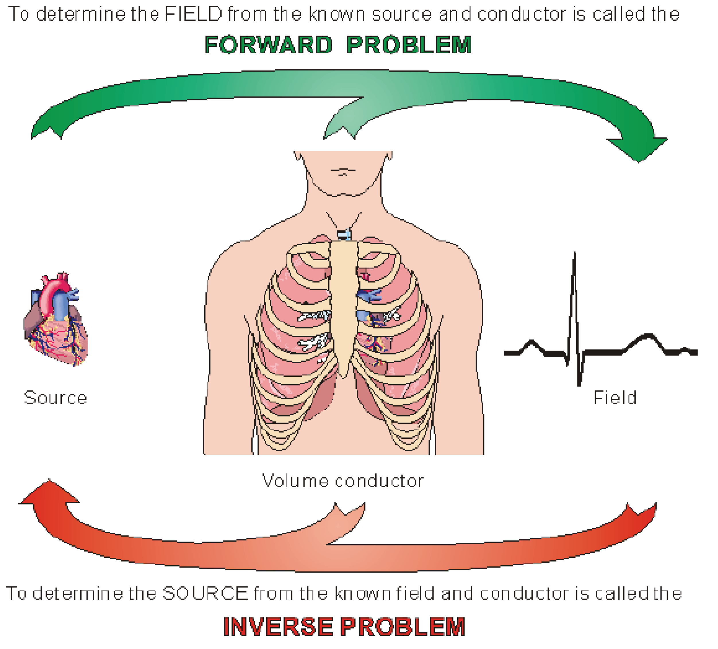
Figure 2.
Block diagram of Inverse Problem solution.
Disclaimer/Publisher’s Note: The statements, opinions and data contained in all publications are solely those of the individual author(s) and contributor(s) and not of MDPI and/or the editor(s). MDPI and/or the editor(s) disclaim responsibility for any injury to people or property resulting from any ideas, methods, instructions or products referred to in the content. |
© 2025 by the authors. Licensee MDPI, Basel, Switzerland. This article is an open access article distributed under the terms and conditions of the Creative Commons Attribution (CC BY) license (http://creativecommons.org/licenses/by/4.0/).
Copyright: This open access article is published under a Creative Commons CC BY 4.0 license, which permit the free download, distribution, and reuse, provided that the author and preprint are cited in any reuse.


