
Submitted:
29 July 2025
Posted:
30 July 2025
You are already at the latest version
Abstract
The electrophysiological modeling of the heart involves two critical challenges: the Forward Problem and the Inverse Problem. While the Forward Problem calculates body surface potentials from known internal cardiac sources, the Inverse Problem seeks to identify the internal bioelectric source distribution from external body surface potential measurements. This study focuses on solving the Inverse Problem using three regularization-based methods: Minimum Norm (MN), Weighted Minimum Norm (WMN), and exact Low Resolution Brain Electromagnetic Tomography (eLORETA). Each method addresses the ill-posed nature of the problem by minimizing error in reconstructing source distributions. The inverse solutions are evaluated using varying electrode configurations and multiple source settings. Results demonstrate that eLORETA provides superior localization accuracy, particularly with single-source scenarios and higher electrode counts. A novel approach to resolve the challenge of boundary point localization is also proposed, enhancing accuracy in problematic regions like the endocardium. Simulations validate the effectiveness of regularization techniques, with eLORETA consistently outperforming MN and WMN methods.
Keywords:
Inverse Problem
; electrophysiology
; regularization
; eLORETA
; Minimum Norm
; Weighted Minimum Norm
; bioelectric source localization
1. Introduction
There are two problems in modeling the electrophysiology of the heart: the Forward Problem and the Inverse Problem [1]. The heart Forward Problem involves designing a model that is capable of determining the field on the surface of known body (conductor) that is generated by electrical-sources inside the heart. Solving the Forward Problem requires the development of electrical models which are capable of describing the bioelectrical criteria of the heart and the body (Figure 1).
The Inverse Problem of the heart electrophysiology can be summarized as how to find detailed information about the distribution of the bioelectric sources in the heart from the electric potentials on the body surface (Body Surface Potential Maps BSPM) or the magnetic fields (MCG) outside the body.
To find the source, given the measured field, there are several approaches that have been used [1]. These include:
- 1-
- An empirical approach based on the recognition of typical signal patterns that are known to be associated with certain source configurations.
- 2-
- Imposition of physiological constraints based on the information available about the anatomy and physiology of the active tissue. This imposes strong limitations on the number of available solutions.
- 3-
- Modeling the source and the volume conductor using simplified models. The source is characterized by only a few degrees of freedom (for instance a single dipole which can be completely determined by three independent measurements).
- 4-
- Examining the lead field pattern, from which the sensitivity distribution of the lead and therefore the statistically most probable source configuration can be estimated.
Where it is difficult to compare one heart model against another [2], validation of the Inverse Problem solution is usually done by comparing results of the system to other real measurements. Real measurements are usually obtained from measuring the volume source potential (usually the Epicardium wall or the Endocardium wall potential) using invasive techniques [3,4,5,6,7,8,9,10,11,12,13,14,15,16,17]. Other methods tend to use simulators of the Forward Problem in the process and then compare the results obtained from the Inverse Model with the ones generated by the Forward Model [18,19,20,21,22,23,24,25].
2. Methods
There is a linear relation between the source and the body surface potential. This relation can be introduced as
where b is the body surface potential vector (dependent variables vector [Mx1]), x is the source vector (independent variables vector [Nx1]), and A is the lead field transfer matrix (MxN) that maps x to b. Thus, solving the Inverse Problem of the heart requires solving the equation
where T is the inverse transfer matrix. Different forms of the transfer matrix A has been introduced in terms of Transmembrance Potential (TMP) instead of Current Destiny vector [26] and it is apparently singular matrix. Thus, finding T cannot be accomplished by regular linear system solution such as Gaussian Elimination.
2.1. Regularization
In general, the Inverse Problem of the heart’s electrophysiology is an ill-posed problem because it breaks one or more of Hadamard conditions of well-posed problem [27,28,29]. As a consequence of the solution not being unique, the error of body surface potential reading being presented in all configurations of the Inverse Problem, and in the multiple pole distribution configuration, the problem becomes strongly underdetermined [22,25] as the number of body surface reading is much less than the number of sources.
Solving the ill-posed Inverse Problem requires reformulating the problem by including some assumptions such as smoothness of solution, which is called the regularization [27,28,29]. Tikhonov regularization [30] is the most common technique used to solve ill-posed problems such as this Inverse Problem is solved by minimizing both the residual error norm and the regularized solution norm. Using this technique the objective function can be written as
where is an estimate of the solution, is the regularization parameter and it is usually determined by L-curve [30,31,32,33] or U-curve [34] and is the regularization matrix.
2.2. The Minimum Norm (MN) Solution
Three methods for solving this function are described here. The Minimum Norm (MN) solution of the Tikhonov regularization is provided by assigning the regularization matrix to the identity matrix. The objective function then becomes:
and the solution of this objective function will be:
2.3. The Weighted Minimum Norm (WMN) Solution
The Weighted MN (WMN) solution is by considering the regularization matrix as a weighting matrix. The objective function then becomes:
and the solution of this objective function will be:
where W is the weighting matrix. The weighting matrix can be smoothed by any smoothing functions such as Laplacian smoothing operator.
2.4. The Low Resolution Brain Electromagnetic Tomography (LORETA) solution
In addition to the MN and WMN solution there is the Low Resolution Brain Electromagnetic Tomography (LORETA) solution [35,36,37,38,39,40] which was developed by Pascual-Marqui. The LORETA methods are linear imaging methods, used mainly to localize the electric neuronal activity in the brain. There are three versions of LORETA methods. The first is the original LORETA, that has good accuracy in localizing test sources even when they are deep and this makes the overall average localization error to be smaller than one voxel. The comparisons between LORETA method and other methods have proven that LORETA has the smallest localization error [36,37,38,41]. The second version is the standardized LORETA (sLORETA) which has zero localization error under ideal conditions of no noise. The last version is the exact LORETA (eLORETA), which is the most advanced version of these models and was derived to include the reading noise error in account making the solution more realistic. The objective matrix form of eLORETA is
where
such that
where H is the average centering operator, and the suffix j means the column number in the matrix as the matrix W is the diagonal matrix, and I is the unity vector.
There are two important matters regarding the Inverse Problem solution. The regularization algorithms are efficient in localizing single primary source [42], but more sources produce inaccurate results. The other matter is that there are some difficulties in localizing sources that are in some zones such as boundaries and Septum of the heart [24].
2.5. Data Generation
The implementation of the Inverse Problem solution is similar to the Forward Problem solution and accomplished using the C/C++ programming language in addition to the OpenGL library to visualize Inverse Model results. Matrix operations in the implementation are performed by some of matrix operations libraries that are found in the ALGLIB site [43]. These libraries have been verified to give correct solution compared with MATLAB.
Localizing the distribution of transmembrance potential is the problem in concern to be solved. Solving the Inverse Problem in terms of transmembrance potentials (TMP) reduces the size of the problem to the third of the current density solution as stated earlier [26]. A low resolution heart geometry that is employed in the solution process by resizing the resolution one [45]. The conduction network of the heart [46,47] could be used in a later stage for modeling the propagation wavefront [48,49]. The number of voxels of the low resolution version of the heart is 960 elements (Figure 2) giving 960 independent variables in the case of TMP and 2880 (960 x 3) independent variables in the current density formulation.
The numbers of electrodes (dependent variables vector) that are used to measure the body surface potential are less than this number [50,51]. The 200, 100, 64 and 32 electrodes configurations were tested for the Inverse Problem solution (Figure 3). The 12-Lead ECG readings are not included because they were not measured with respect to the same reference, and the six electrograms which were measured with respect to WCT are too few to generate a good solution (the system will be extremely underdetermined).
As the number of the independent variables exceeds the number of the dependent variables, this problem is highly underdetermined and due to that, three regularization methods are used for localizing the primary sources locations inside the ventricles, namely, the Minimum Norm (MN), the Weighted Minimum Norm, (WMN) and the eLORETA. The matrix multiplication which is of O(N3) is the operation of the highest computing cost among other matrix operations where N is the number of elements in the matrix. This makes TMP’s formulation take the advantage over the current density formulation in reducing the computation cost.
The MN method has less matrix operations among all other methods including the WMN and the eLORETA, requiring less processing time. The eLORETA method requires the largest time as it contains several matrix multiplications. Another factor that affects the processing time is the number of electrodes readings (the dependent variables), and for example, with the MN method, 32 electrodes require a few minutes for solving the problem, while 200 electrodes it requires double that time.
2.6. Localization Problem of Boundary Points
Localizing the boundary points (including both external heart boundary, and blood volume boundary) that act as primary sources points is not accurate in most of cases, especially the ones located in the Endocardium of the ventricles. A novel approach is introduced to solve this problem, where small leakage currents between boundary points of the heart and neighboring non-excitable points are assumed. The solution then includes more points, which make the heart’s boundary points becomes sub-boundary points and so the problem is transferred to these added points which will never be activated. This provided a solution to the problem of localizing the activation points in some parts in the heart [24].
3. Results
For evaluating the correctness of the inverse solution, thousands of runs for each regularization method was performed. It was reported that the regularization methods are successful in determining single pacing point [42]. However, multiple pacing points were also included to evaluate the power of each of these regularization methods in determining such cases. The number of body surface electrodes is other factor that is used to in this evaluation as well. Some initial activation points are assigned to the heart model and the BSPM is being generated. The resultant BSPM is used as an input to recover the location of the activation points.
Selection of the regularization parameter for all of the used methods is accomplished by testing some small values and choice of the one that provide the best results. The weighting matrix of the eLORETA converges after few numbers of iterations (5 to 7). The evaluation of the efficiency of the each of these regularization methods is accomplished by comparing the recovered activation points from each of them with the original assigned activation points.
When an activation point (red pixel) is assigned as a volume source inside the heart Myocardium (Original), the Forward Model is used to generate the BSPM that corresponds to this activation. The generated BSPM is then used as the field input to the regularization method. It is clear from Figure 4 that these regularization methods are capable to determine an approximate location of the original activation point. The red color introduces positive component, the blue color introduces negative component and the green color introduces the zero component. The eLORETA is found to be the best method among these three methods that has excellent coloration with the original source points.
Two thousands different settings for each method were used to calculate the Inverse Problem solution. Each setting includes primary sources with random location ranging from one to five sources and body surface electrodes of 200, 100, 64 and 32 electrodes. Each 100 of these settings have similar number of primary sources and body surface electrodes, but with random locations for the primary sources. The MN results required almost 15 hours on a Pentium 4 – 1.7 GHz processor with 2GB RAM, while the WMN results took about 30 hours and the eLORETA method about 80 hours.
To measure the compatibility with the original pacing points (primary sources), the CC and the RE were calculated together with and the Mean and the Standard Deviation for the CC and the RE. Table 1 shows the mean and the standard deviation of each group of settings. It was found that the best localization results are produced when the number of primary sources equal to one and the more the number of electrodes the more the accurate the results (Figure 5, Figure 6, Figure 7, Figure 8, Figure 9, Figure 10, Figure 11 andFigure 12). The eLORETA method was found to be the best method among the three methods for localizing the original source.
Finally, regularization methods are successful in determining a single primary source, but have less ability to localize multiple primary sources. The number of body surface readings affect the correctness of the regularization method, as the greater number or body surface electrodes produces better results. Identifying boundary pacing sites is done accurately by assuming a small leakage current to the surrounding surface and includes these points in the regularization process. The eLORETA method produces better results in the Inverse Problem solution than the MN or the WMN methods.
4. Conclusion
Solving the Inverse Problem of cardiac electrophysiology requires handling its inherently ill-posed nature through regularization techniques. This study has demonstrated that the MN, WMN, and eLORETA methods can successfully localize single internal sources based on body surface potentials, with eLORETA showing the highest accuracy and robustness across different test cases. While MN is computationally efficient, its accuracy is lower compared to eLORETA, especially in multi-source scenarios. The number of body surface electrodes significantly influences solution accuracy, with more electrodes yielding better localization results. Additionally, a novel boundary localization strategy—assuming small leakage currents to neighboring non-excitable points—significantly improves the accuracy in localizing activation points near the heart's boundary and septal regions. Despite limitations in multi-source localization, eLORETA offers a promising and more realistic approach to solving the cardiac Inverse Problem.
References
- J. Malmivuo and R. Plonsey "Bioelectromagnetism: Principles and Applications of Bioelectric and Biomagnetic Fields" Oxford Univ. Press, 1st Ed., (1995); ISBN: 0195058232.
- M. Lorange, and R. M. Gulrajani "A computer Heart Model Incorporating Anisotropic Propagation" Journal of Electrocardiology, (1993);26(4):245-261. [CrossRef]
- M. Seger "Modeling the Electrical Function of the Human Heart", Ph.D. Thesis, Institute of Biomedical Engineering, University for Health Sciences, Medical Informatics and Technology, Austria (2006).
- D.H. Brooks and R.S. MacLeody "Electrical Imaging of the Heart: Electrophysical Underpinnings and Signal Processing Opportunities" IEEE Signal Processing, (1996); 14(1):24-42.
- C. Hintermuller "Development of a Multi-Lead ECG Array for Noninvasive Imaging of the Cardiac Electrophysiology", Ph.D. Thesis, Institute of Biomedical Engineering, University for Health Sciences, Medical Informatics and Technology,Austria, (2006).
- BJ Messinger-Rapport and Y. Rudy "Noninvasive recovery of epicardial potentials in a realistic heart- torso geometry.Normal sinus rhythm" American Heart Association (1990);66;1023-1039. [CrossRef]
- H.S. Oster, B.Taccardi, R.L. Lux, P.R. Ershler and Y. Rudy "Electrocardiographic Imaging : Noninvasive Characterization of Intramural Myocardial Activation From Inverse-Reconstructed Epicardial Potentials and Electrograms" American Heart Association (1998);97:1496-1507. [CrossRef]
- T. Berger, G. Fischer, B. Pfeifer, R. Modre, F. Hanser,T. Trieb, F. X. Roithinger, M. Stuehlinger, O. Pachinger,B. Tilg, and F. Hintringer "Single-Beat Noninvasive Imaging of Cardiac Electrophysiology of Ventricular Pre-Excitation" J. Am. Coll. Cardiol. (2006);48:2045-2052. [CrossRef]
- L. Cheng "Non-Invasive Electrical Imaging of the Heart", Ph.D. Thesis, The University of Auckland, New Zealand (2001).
- C. Ramanathan, P. Jia, R. Ghanem, D. Calvetti, and Y. Rudy "Noninvasive Electrocardiographic Imaging (ECGI):Application of the Generalized Minimal Residual (GMRes) Method" Ann. Biomed. Eng. 2003; 31(8): 981–994. [CrossRef]
- R. N. Ghanem,P. Jia, C. Ramanathan, K. Ryu, A. Markowitz, and Y. Rudy "Noninvasive Electrocardiographic Imaging (ECGI): Comparison to intraoperative mapping in patients" Heart Rhythm. 2005; 2(4): 339–354. [CrossRef]
- A. Intini, R. N. Goldstein, P. Jia, C. Ramanathan,K.Ryu, B.Giannattasio,R.Gilkeson,B.S. Stambler,P. Brugada,W. G. Stevenson, Y. Rudy, and A. L. Waldo "Electrocardiographic imaging (ECGI), a novel diagnostic modality used for mapping of focal left ventricular tachycardia in a young athlete" Heart Rhythm. 2005; 2(11): 1250–1252. [CrossRef]
- P. Jia,C. Ramanathan,R.N. Ghanem,K. Ryu,N. Varma,and Y. Rudy "Electrocardiographic imaging of cardiac resynchronization therapy in heart failure: Observation of variable electrophysiologic responses" Heart Rhythm. 2006; 3(3): 296–310. [CrossRef]
- R.N. Ghanem, C. Ramanathan, P.Jia, and Y. Rudy "Heart-Surface Reconstruction and ECG Electrodes Localization Using Fluoroscopy, Epipolar Geometry and Stereovision:Application to Noninvasive Imaging of Cardiac Electrical Activity" IEEE Trans. Med. Imaging. 2003; 22(10): 1307–1318. [CrossRef]
- T.Berger, F.Hintringer, G. Fischer, "Noninvasive Imaging of Cardiac Electrophysiology" Indian Pacing and Electrophysiology Journal, 2007; 7(3): 160-165.
- C. Ramanathan, R.N. Ghanem, P. Jia, K. Ryu, and Y. Rudy "Noninvasive electrocardiographic imaging for cardiac electrophysiology and arrhythmia" Nat Med. 2004; 10(4): 422–428. [CrossRef]
- S. Ghosh and Y. Rudy "Accuracy of Quadratic Versus Linear Interpolation in Noninvasive Electrocardiographic Imaging (ECGI)" Ann. Biomed. Eng. 2005; 33(9): 1187–1201. [CrossRef]
- M. Seger, R. Modre, B. Pfeifer, C. Hintermuller and B. Tilg "Non-invasive Imaging of Atrial Flutter" Computers in Cardiology (2006);33:601-604.
- X. Zhang, I. Ramachandra, Z. Liu, B. Muneer, S.M. Pogwizd, and B. He "Noninvasive three-dimensional electrocardiographic imaging of ventricular activation sequence" Am J Physiol Heart Circ Physiol (2005); 289: H2724–H2732. [CrossRef]
- C.G. Xanthis, P.M. Bonovas, and G.A. Kyriacou "Inverse Problem of ECG for Direrent Equivalent Cardiac Sources" PIERS Online, 2007; 3(8): 1222-1227.
- B. He, G.Li, and X. Zhang "Noninvasive Imaging of Cardiac Transmembrane Potentials Within Three-Dimensional Myocardium by Means of a Realistic Geometry Anisotropic Heart Model" IEEE Trans. Biomed. Eng. (2003); 50(10): 1190-1202. [CrossRef]
- B. He, and D. Wu "Imaging and Visualization of 3-D Cardiac Electric Activity" IEEE Tran. Inf Tech. Biomed. 2001; 5(3): 181-186. [CrossRef]
- G. Li, X. Zhang, J. Lian, and B. He "Noninvasive Localization of the Site of Origin of Paced Cardiac Activation in Human by Means of a 3-D Heart Model" IEEE Trans. Biomed. Eng. (2003); 50(9): 1117-1120. [CrossRef]
- Z. Liu, C. Liu, and B. He "Noninvasive Reconstruction of Three-Dimensional Ventricular Activation Sequence From the Inverse Solution of Distributed Equivalent Current Density" IEEE Trans. Med. Imag. (2006); 25(10): 1307-1318. [CrossRef]
- B. He, C. Liu ,and Y. Zhang "Three-Dimensional Cardiac Electrical Imaging From Intracavity Recordings" IEEE Trans. Biomed. Eng. (2007); 54(8): 1454-1460. [CrossRef]
- ELAFF I., “Formulation of the Transfer Matrix of the Invers Electrophysiology of the Heart Activation Inside Homogeneous and Inhomogeneous Volume Conductor”. Preprints 2025, 2025072286.
- R.D. Pascual-Marqui "Review of Methods for Solving the EEG Inverse Problem" Intr. J. Bioelectromagnetism (1999); 1(1): 75-86.
- R.S. MacLeod and D.H. Brooks "Recent Progress in Inverse Problems in Electrocardiology" (1998) University of Utah. [CrossRef]
- M.J.M. Cluitmans "Investigation of Electrocardiographic Imaging as a Medical Tool" Electrocardiographic Imaging as a Medical Tool, 2007.
- M. Burger "Inverse Problems" Lecture Notes, The Department of Computational and Applied Mathematics, University of Münster, (2007).
- G. Rodriguez "An algorithm for estimating the optimal regularization parameter by the L-curve" Rendiconti di Matematica, Serie VII (2005); 25: 69-84.
- S. Oraintara, W.C. Karl, D.A. Castanon and T.Q. Nguyen "A Method for Choosing the Regularization Parameter in Generalized Tikhonov Regularized Linear Inverse Problems" Multi-Dimensional Signal Processing Laboratory, Boston University. [CrossRef]
- M.E.Kilmer and D.P. O'Leary "Choosing Regularization Parameter in Iterative Methods for ill-posed Problems" SIAM J. on Matrix Analy. and App., (2000); 22(4): 1204 - 1221. [CrossRef]
- D. Krawczyk-Stando, M. Rudnicki "Regularization Parameter Selection in Discrete ill–Posed Problems —The use of the U–Curve" Int. J. Appl. Math. Comput. Sci., (2007); 17(2): 157–164.
- LORETA Site "https://www.uzh.ch/keyinst/loreta", July 2025.
- R.D. Pascual-Marqui, C.M. Michel, and D. Lehman "Low resolution electromagnetic tomography: A new method for localizing electrical activity in the brain" Inter. J. of Psych, (1994); 18: 49-65. [CrossRef]
- R.D. Pascual-Marqui, M. Esslen, K. Kochi and D. Lehman "Functional imaging with low resolution brain electromagnetic tomography (LORETA): a review" Methods & Findings in Experimental & Clinical Pharmacology, (2002); 24(C):91-95.
- R.D. Pascual-Marqui "Review of Methods for Solving the EEG Inverse Problem" Inter. J. of Bioelectromagnetism, (1999); 1(1):75-86.
- R.D. Pascual-Marqui "Discrete, 3D distributed linear imaging methods of electric neuronal activity. Part 1: exact, zero error localization" The KEY Institute for Brain-Mind Research, University Hospital of Psychiatry Lenggstr, Switzerland, (2007); arXiv:0710.3341 [math-ph].
- R.D. Pascual-Marqui "Standardized low resolution brain electromagnetic tomography (sLORETA): technical details" Methods & Findings in Experimental & Clinical Pharmacology (2002); 24(D):5-12.
- J.P. Russell and Z.J. Koles "A Comparison of LORETA and the Borgiotti-Kaplan Beamformer in Simulated EEG Source Localization with a Realistic Head Model" Inter. J. of Bioelectromagnetism (2007); 9(2): 97-98.
- R.G. de Peralta Menendez and S.G. Andino "Comparison of Algorithms for the Localization of Focal Sources: Evaluation with Simulated Data and Analysis of Experimental Data" Inter. J. of Bioelectromagnetism (IJBEM), (2002); 4(1): online.
- ALGLIB Site “http://www.alglib.net/”, July 2025.
- G.K. Massing, and T.N. James "Anatomical Configuration of the His Bundle and Bundle Branches in the Human Heart" Circ. (1976); 53(4):609-621. [CrossRef]
- Elaff, I. “Modeling of the Human Heart in 3D Using DTI Images”, World Journal of Advanced Engineering Technology and Sciences, 2025, 15(02), 2450-2459. [CrossRef]
- El-Aff, I.A.I. "Extraction of human heart conduction network from diffusion tensor MRI" The 7th IASTED International Conference on Biomedical Engineering, 217-22. [CrossRef]
- Elaff, I. “Modeling the Human Heart Conduction Network in 3D using DTI Images”, World Journal of Advanced Engineering Technology and Sciences, 2025, 15(02), 2565–2575. [CrossRef]
- Elaff, I. "Modeling of realistic heart electrical excitation based on DTI scans and modified reaction diffusion equation" Turkish Journal of Electrical Engineering and Computer Sciences: 2018, 26(3): Article 2. [CrossRef]
- Elaff, I. “Modeling of The Excitation Propagation of The Human Heart”, World Journal of Biology Pharmacy and Health Sciences, 2025, 22(02): 512–519. [CrossRef]
- Elaff, I. “Modeling of 3D Inhomogeneous Human Body from Medical Images”, World Journal of Advanced Engineering Technology and Sciences. 2025, 15(02): 2010-2017. [CrossRef]
- Elaff, I. “Modeling of the Body Surface Potential Map for Anisotropic Human Heart Activation”, Research Square, 2025. [CrossRef]
Figure 1.
The Forward and the Inverse Problems of the heart electrophysiology [1].
Figure 1.
The Forward and the Inverse Problems of the heart electrophysiology [1].
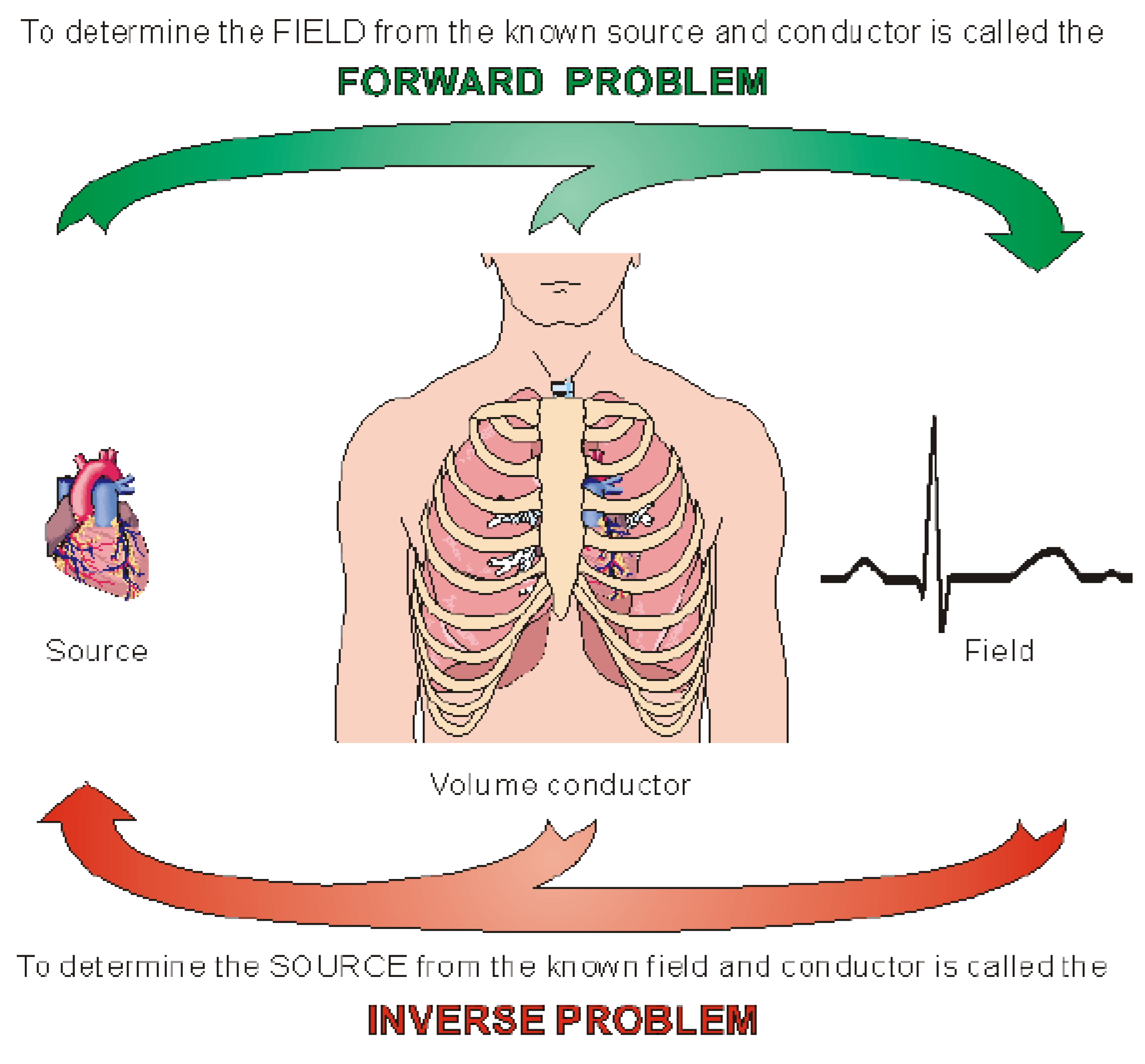
Figure 2.
Slices of Low Resolution heart that contains 960 elements.
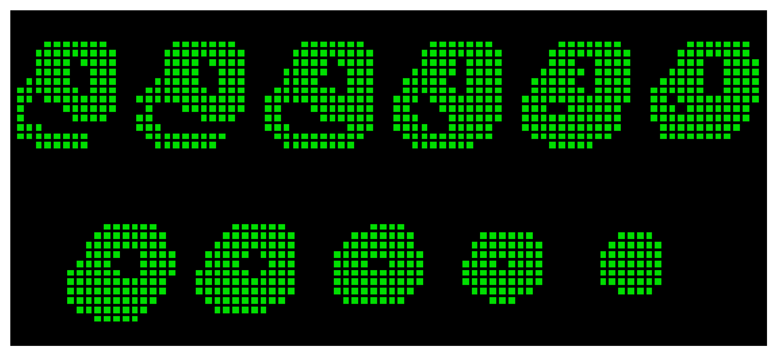
Figure 3.
Multi- electrodes setting. (a) 32 electrodes, (b) 64 electrodes, (c) 100 electrodes and (d) 200 electrodes.
Figure 3.
Multi- electrodes setting. (a) 32 electrodes, (b) 64 electrodes, (c) 100 electrodes and (d) 200 electrodes.
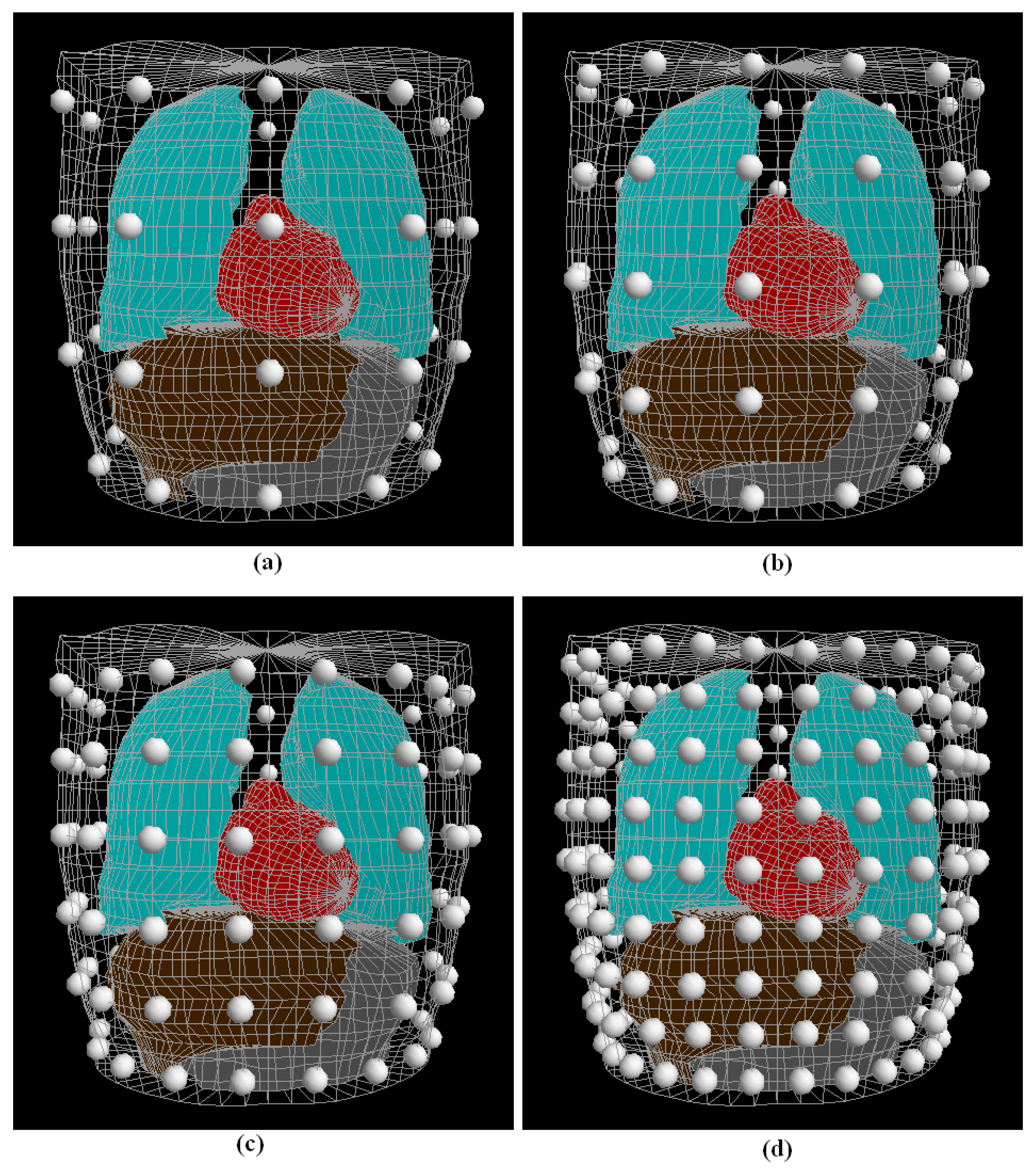
Figure 4.
Comparison between the results of MN, WMN and eLORETA that are generated by one source.
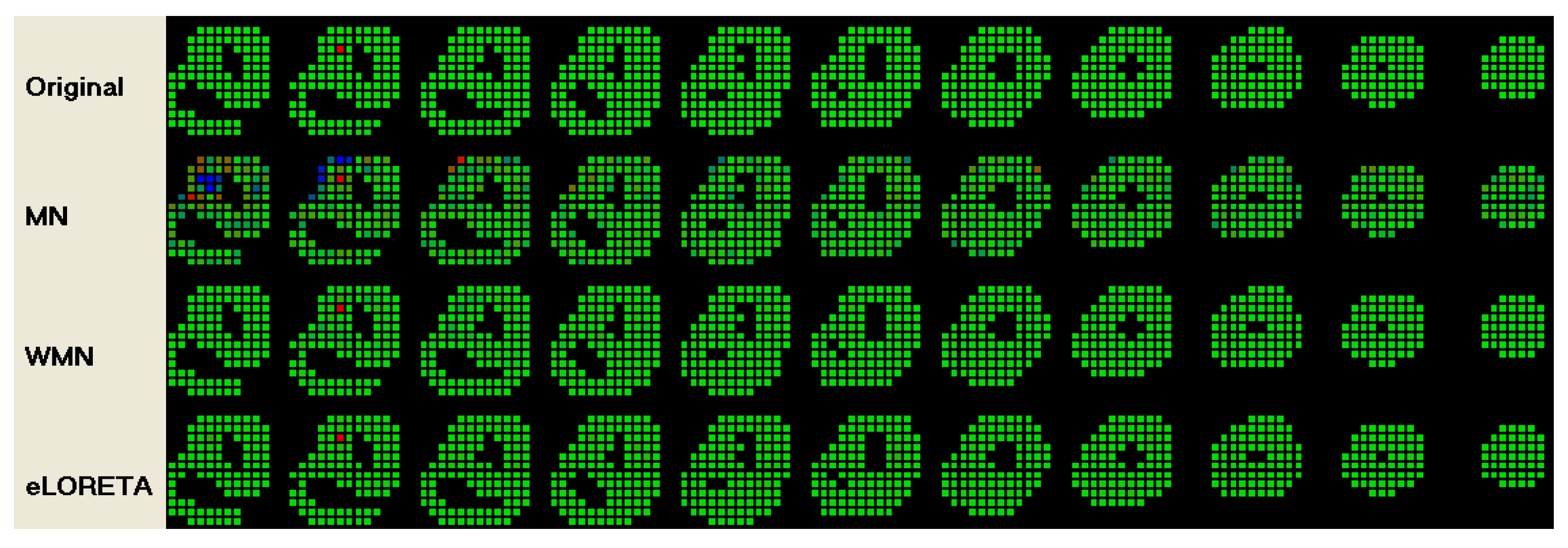
Figure 5.
Comparison between some regularization methods: One Primary sources and 200 body surface electrodes.
Figure 5.
Comparison between some regularization methods: One Primary sources and 200 body surface electrodes.

Figure 6.
Comparison between some regularization methods: Two Primary sources and 200 body surface electrodes.
Figure 6.
Comparison between some regularization methods: Two Primary sources and 200 body surface electrodes.
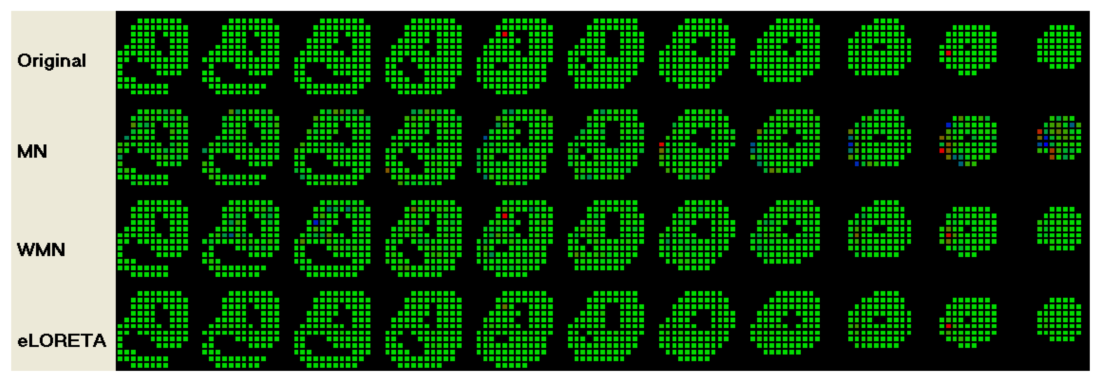
Figure 7.
Comparison between some regularization methods: Three Primary sources and 200 body surface electrodes.
Figure 7.
Comparison between some regularization methods: Three Primary sources and 200 body surface electrodes.
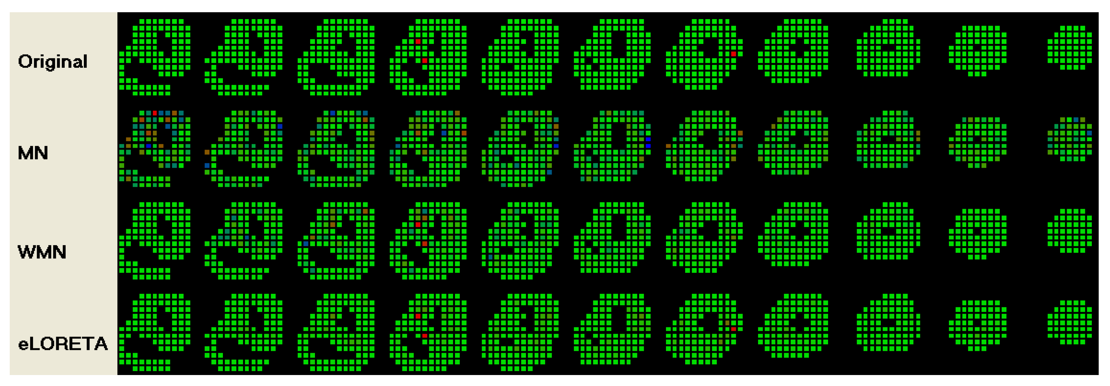
Figure 8.
Comparison between some regularization methods: Four Primary sources and 200 body surface electrodes.
Figure 8.
Comparison between some regularization methods: Four Primary sources and 200 body surface electrodes.
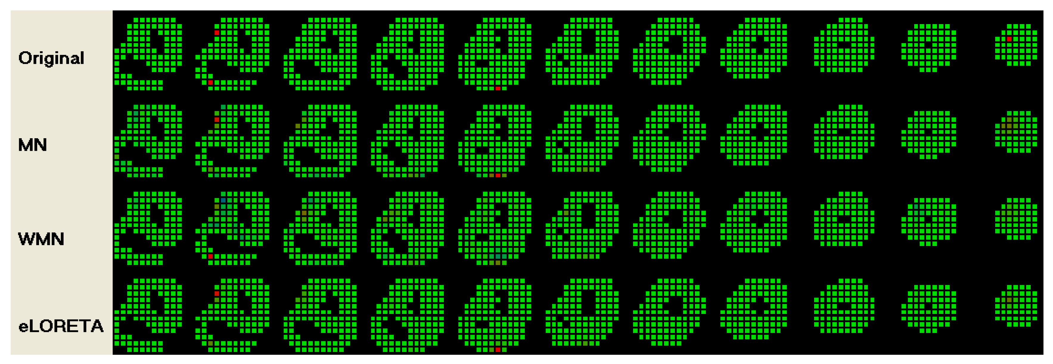
Figure 9.
Comparison between some regularization methods: Five Primary sources and 200 body surface electrodes.
Figure 9.
Comparison between some regularization methods: Five Primary sources and 200 body surface electrodes.
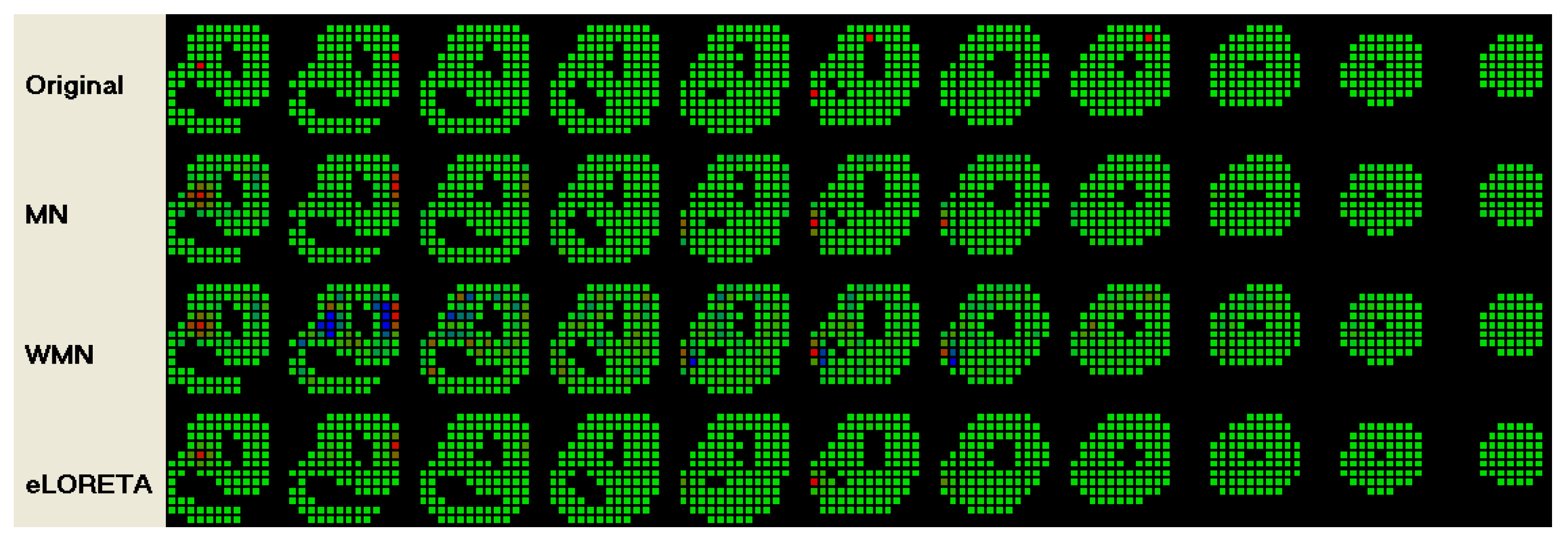
Figure 10.
Comparison between some regularisation methods: One Primary sources and 100 body surface electrodes.
Figure 10.
Comparison between some regularisation methods: One Primary sources and 100 body surface electrodes.
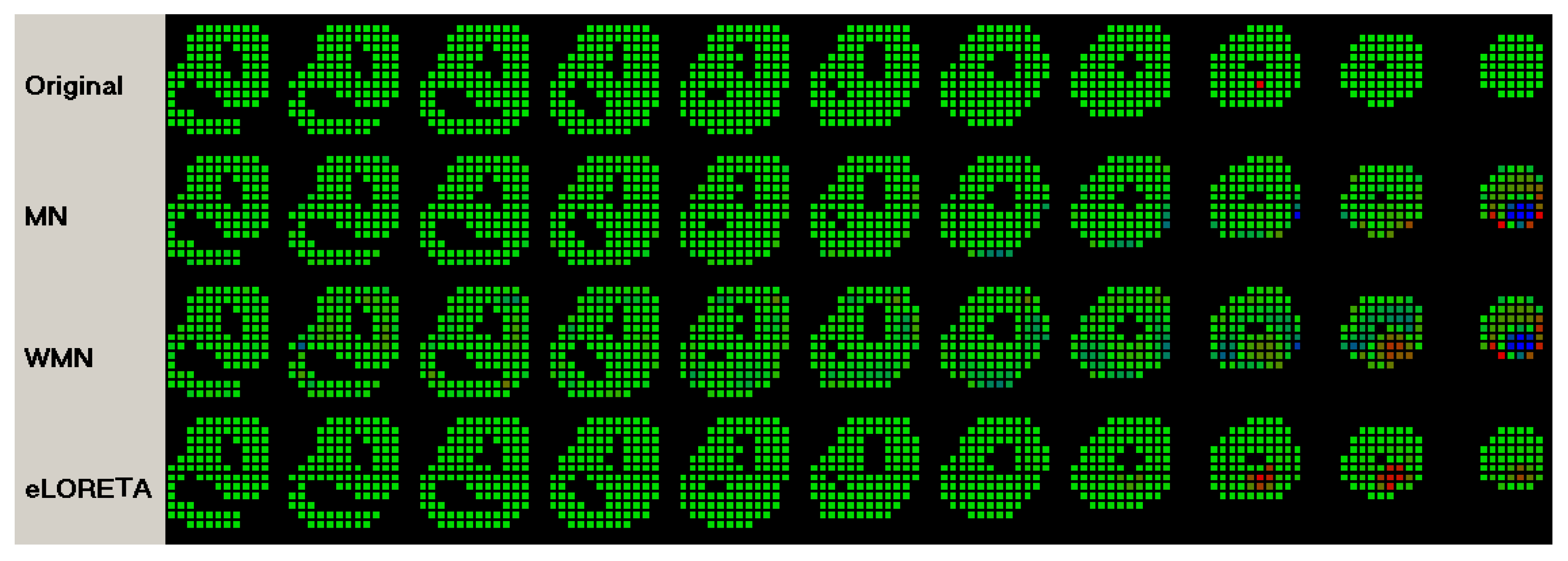
Figure 11.
Comparison between some regularisation methods: One Primary sources and 64 body surface electrodes.
Figure 11.
Comparison between some regularisation methods: One Primary sources and 64 body surface electrodes.
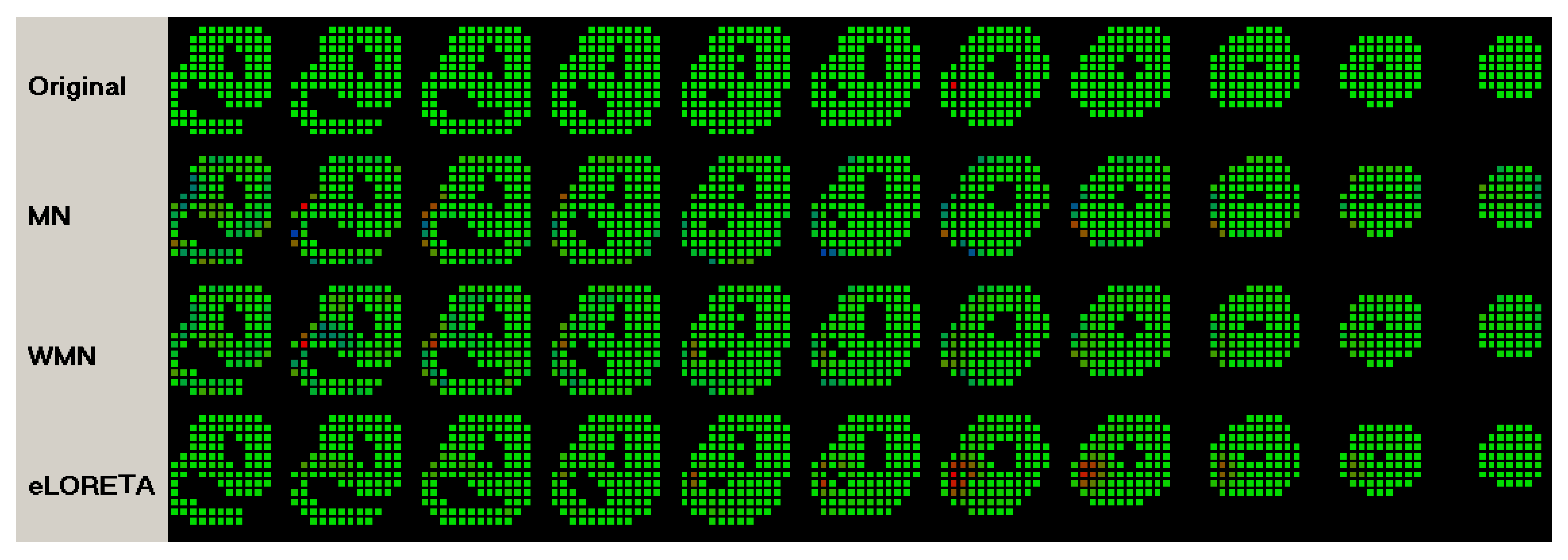
Figure 12.
Comparison between some regularisation methods: One Primary sources and 32 body surface electrodes.
Figure 12.
Comparison between some regularisation methods: One Primary sources and 32 body surface electrodes.
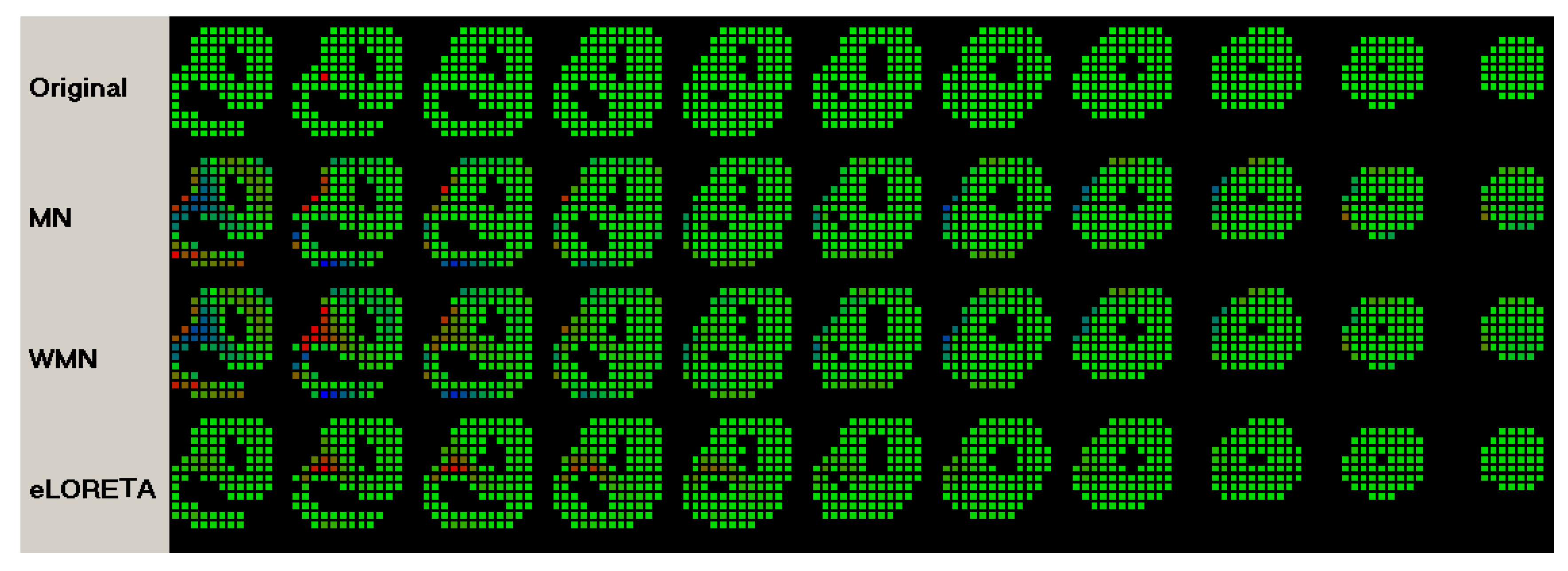

Table 1.
Comparability between different regularization methods and the original settings using different configurations.
Table 1.
Comparability between different regularization methods and the original settings using different configurations.
| # of | eLORETA | WMN | MN | ||||
| Sources | Electrodes | CC | RE | CC | RE | CC | RE |
| 1 | 200 | 0.813 ±0.076 |
0.712 ±0.210 |
0.305 ±0.170 |
3.277 ±1.329 |
0.353 ±0.261 |
3.543 ±2.324 |
| 2 | 200 | 0.657 ±0.104 |
0.830 ±0.170 |
0.279 ±0.125 |
2.486 ±0.910 |
0.364 ±0.197 |
1.996 ±1.195 |
| 3 | 200 | 0.606 ±0.109 |
0.826 ±0.126 |
0.312 ±0.097 |
1.946 ±0.644 |
0.408 ±0.172 |
1.424 ±0.880 |
| 4 | 200 | 0.575 ±0.104 |
0.842 ±0.110 |
0.286 ±0.086 |
1.804 ±0.486 |
0.376 ±0.159 |
1.406 ±0.786 |
| 5 | 200 | 0.563 ±0.095 |
0.836 ±0.079 |
0.298 ±0.072 |
1.609 ±0.397 |
0.404 ±0.134 |
1.168 ±0.480 |
| 1 | 100 | 0.518 ±0.144 |
1.771 ±0.610 |
0.229 ±0.133 |
4.229 ±2.155 |
0.232 ±0.221 |
3.933 ±2.164 |
| 2 | 100 | 0.432 ±0.108 |
1.420 ±0.440 |
0.234 ±0.096 |
2.667 ±1.231 |
0.257 ±0.172 |
2.559 ±1.566 |
| 3 | 100 | 0.419 ±0.099 |
1.177 ±0.268 |
0.225 ±0.070 |
2.087 ±0.569 |
0.298 ±0.133 |
1.634 ±0.725 |
| 4 | 100 | 0.385 ±0.114 |
1.157 ±0.262 |
0.224 ±0.077 |
1.945 ±0.627 |
0.279 ±0.128 |
1.654 ±0.899 |
| 5 | 100 | 0.393 ±0.105 |
1.079 ±0.167 |
0.232 ±0.073 |
1.721 ±0.422 |
0.296 ±0.112 |
1.359 ±0.393 |
| 1 | 64 | 0.375 ±0.110 |
2.699 ±0.908 |
0.203 ±0.119 |
4.419 ±1.803 |
0.181 ±0.156 |
3.954 ±1.754 |
| 2 | 64 | 0.313 ±0.084 |
2.027 ±0.665 |
0.181 ±0.086 |
3.345 ±1.380 |
0.175 ±0.117 |
3.045 ±1.347 |
| 3 | 64 | 0.285 ±0.082 |
1.629 ±0.407 |
0.184 ±0.077 |
2.502 ±1.000 |
0.201 ±0.097 |
2.244 ±1.005 |
| 4 | 64 | 0.282 ±0.076 |
1.509 ±0.374 |
0.185 ±0.066 |
2.191 ±0.756 |
0.203 ±0.090 |
1.963 ±0.766 |
| 5 | 64 | 0.276 ±0.065 |
1.436 ±0.297 |
0.194 ±0.062 |
1.918 ±0.512 |
0.225 ±0.074 |
1.665 ±0.449 |
| 1 | 32 | 0.277 ±0.080 |
3.784 ±1.270 |
0.150 ±0.107 |
4.860 ±1.662 |
0.136 ±0.131 |
4.373 ±1.740 |
| 2 | 32 | 0.230 ±0.060 |
2.727 ±0.895 |
0.146 ±0.079 |
3.651 ±1.356 |
0.142 ±0.099 |
3.295 ±1.425 |
| 3 | 32 | 0.215 ±0.047 |
2.264 ±0.627 |
0.152 ±0.069 |
2.902 ±0.984 |
0.155 ±0.085 |
2.662 ±0.953 |
| 4 | 32 | 0.211 ±0.044 |
1.954 ±0.493 |
0.157 ±0.051 |
2.384 ±0.645 |
0.164 ±0.063 |
2.226 ±0.689 |
| 5 | 32 | 0.207 ±0.049 |
1.853 ±0.410 |
0.162 ±0.057 |
2.258 ±0.648 |
0.171 ±0.066 |
2.116 ±0.637 |
Disclaimer/Publisher’s Note: The statements, opinions and data contained in all publications are solely those of the individual author(s) and contributor(s) and not of MDPI and/or the editor(s). MDPI and/or the editor(s) disclaim responsibility for any injury to people or property resulting from any ideas, methods, instructions or products referred to in the content. |
© 2025 by the authors. Licensee MDPI, Basel, Switzerland. This article is an open access article distributed under the terms and conditions of the Creative Commons Attribution (CC BY) license (http://creativecommons.org/licenses/by/4.0/).
Copyright: This open access article is published under a Creative Commons CC BY 4.0 license, which permit the free download, distribution, and reuse, provided that the author and preprint are cited in any reuse.


