
Submitted:
12 June 2025
Posted:
13 June 2025
You are already at the latest version
Abstract
This study evaluates the contribution of individual organs to the Body Surface Potential Map (BSPM) generated during ventricular activation. The human torso was modeled as an inhomogeneous volume conductor using CT data, and the heart was treated as an anisotropic volume source based on Diffusion Tensor Imaging (DTI). The ventricular conduction system was also extracted from DTI scans. Excitation propagation was simulated using the Monodomain Reaction-Diffusion Equation (MD-RDE), and the resulting BSPM was computed. By selectively removing specific organs from the torso model and comparing BSPMs using correlation coefficient and relative error metrics, the study identifies the relative influence of each organ. Results confirm that the blood volume within the ventricles has the greatest impact on BSPM accuracy, with the bones, lungs, and liver having lesser but measurable effects.
Keywords:
cardiac electrophysiology
; body surface potential map (BSPM)
; monodomain reaction-diffusion equation (MD-RDE)
; inhomogeneous body
1. Introduction
The conduction system defines the primary excitation sites within the heart’s myocardium, which subsequently initiate the propagation of electrical activity throughout the myocardium. The resulting potential differences between activated and non-activated regions inside the heart create volume current sources that give rise to both electric potentials on the body surface and magnetic fields detectable outside the body [1].
The body may be represented as either a homogeneous or an inhomogeneous volume conductor. In the homogeneous model, all organs—including the blood volume within the ventricles—are assumed to share identical physical properties. Conversely, the inhomogeneous model assigns distinct parameters to each organ. As demonstrated by Gulrajani and Mailloux [2], the body’s inhomogeneity significantly influences the resulting surface potentials, with the blood mass identified as the most impactful factor.
In reality, all organs exhibit anisotropic properties. Tissues like skeletal muscles display pronounced anisotropy, whereas others, such as the liver and lungs, are nearly isotropic [1]. Accurately modeling organ anisotropy demands extensive data detailing each organ’s structural composition. Nevertheless, treating organs as isotropic materials is a reasonable approximation that simplifies the modeling process [1]. Some models represent the volume conductor—the body—using simplified geometric shapes; however, the most commonly adopted approach is the realistic torso shape. Within this framework, the torso is modeled either as a homogeneous volume conductor [2,3,4,5,6,7,8] or, more frequently, as an inhomogeneous volume conductor [9,10,11,12,13,14,15,16,17,18,19,20].
The majority of models utilize the body surface potential [21,22,23,24,25,26,27,28,29,30], while a smaller number focus on the heart’s magnetic field map [31]. Some models, however, incorporate both electric and magnetic fields in their analysis [3,7,32,33]. This study focuses on measuring the contribution of each organ to the BSPM of ventricle activation.
2. Methods
2.1. The Human Torso and the Human Heart Modeling
Human torso (Figure 1) has been modeled as inhomogeneous volume conductor using CT-Scans [20] and human heart is modeled as anisotropic volume source [34] using DTI images. The ventricles conduction network is extracted as well based on DTI images [35,36].
Figure 1.
Human Torso [20].
Figure 1.
Human Torso [20].
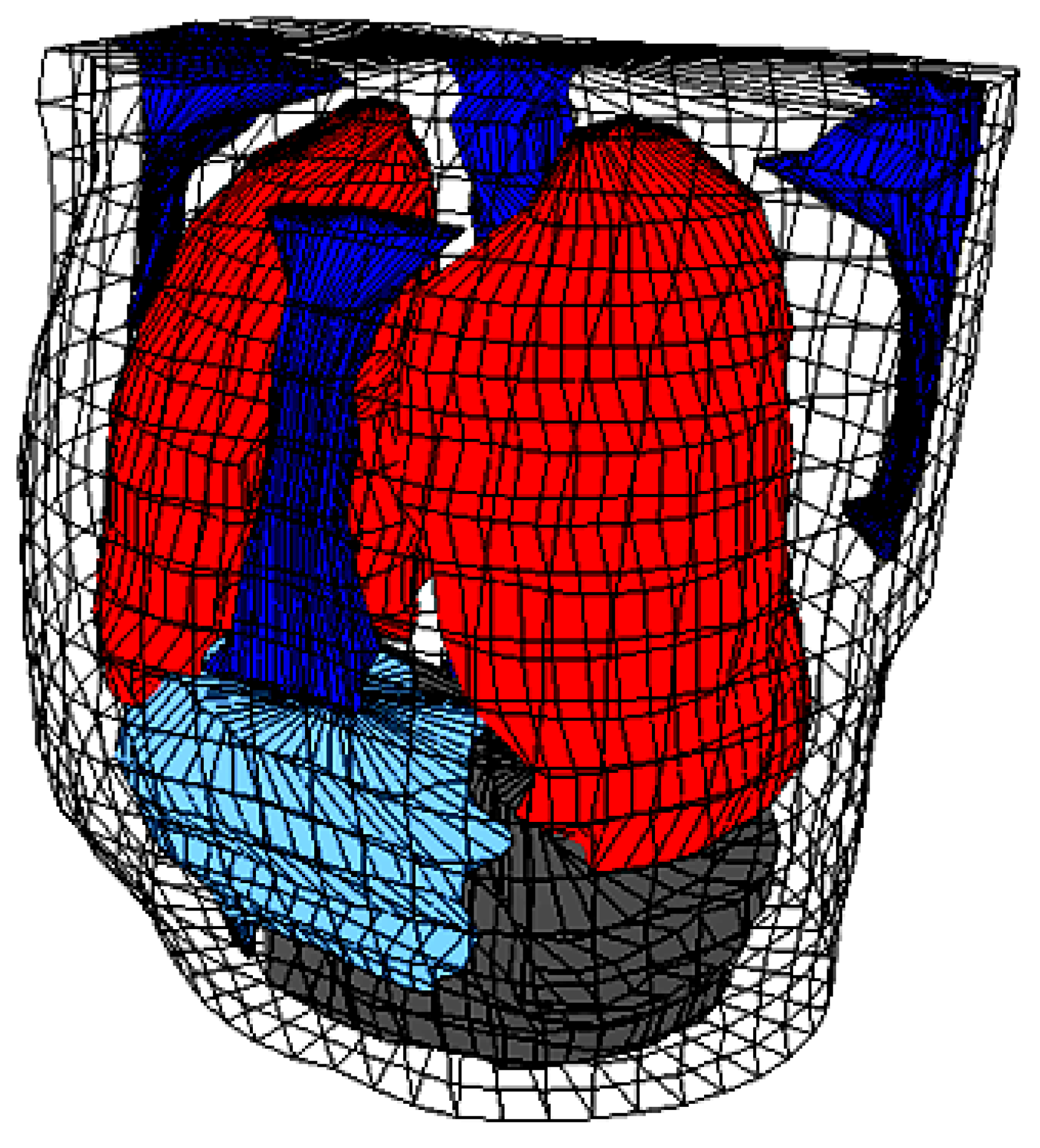

Table 1.
Different values of tissues and organs resistivity and conductivities [20].
Table 1.
Different values of tissues and organs resistivity and conductivities [20].
| Organ/Tissue | Resistivity (Ωcm) |
Conductivity (mS/mm) |
|---|---|---|
| Skeletal muscle | 400 | 25 |
| Fats | 2000 | 5 |
| Bone | 2000 | 5 |
| Liver | 600 | 16.7 |
| Left lung, right lung | 1325 | 7.5 |
| Blood masses | 150 | 66.7 |
| Other tissues and organs | 460 | 21.7 |
| Heart muscle | 450 | 22.2 |
2.2. Heart Activation Isochrones
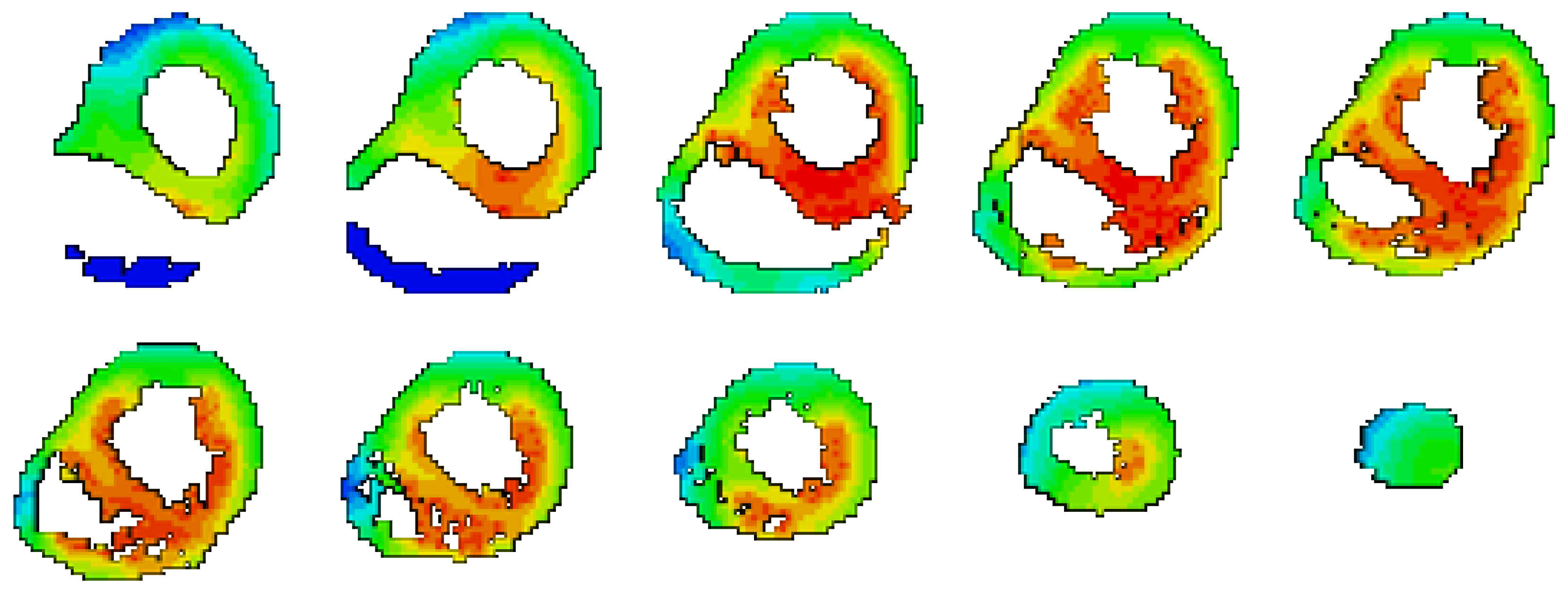
Excitation propagation of the heart is modeled in tissue scale based on Monodomain Reaction Diffusion Equation (MD-RDE) [37,38,39].
Figure 2.
The isochrones for the excitation propagation of the heart when it is considered an Anisotropic material [38].
Figure 2.
The isochrones for the excitation propagation of the heart when it is considered an Anisotropic material [38].
2.3. Body Surface Potential Map
3. Results
It was reported the blood volume inside the ventricles has a significant effect on the BSPM, and this fact is verified in this section. The effects of other organs over the BSPM are also considered by removing each organ from the body and recalculating the BSPM. The case of homogeneous body is also taken into consideration. The difference is considered by comparing the reference configuration (the heart is considered anisotropic material and the body as an inhomogeneous volume conductor) to each of the following configurations:
- Removing Bones only.
- Removing Other organs only.
- Removing Liver only.
- Removing Lungs only.
- Removing Blood Volume only.
- Homogeneous body.
The results of Coefficient Correlation (CC) and Relative Error (RE) for these different configurations are presented in Table 2, and Table 3 respectively, presented graphically in Figure 4 and Figure 5.
It was found the largest difference occurs when removing the blood volume from the BSPM calculations, and then it almost produces an output similar to the homogeneous body case. Removing the Other organs only has slight effect on the results. According to the previous analysis, the effects of organs are arranged in a descending order from the highest effect to the lowest according to the mean value of RE as follows:
- The Blood Volume.
- The Bones.
- The Lungs.
- The Liver.
- Any Other organs.
4. Conclusions
The simulation results clearly show that the blood volume inside the ventricles plays the most significant role in shaping the BSPM, nearly equating the error produced when assuming a homogeneous torso. The bones, lungs, and liver also contribute to BSPM accuracy, but to a lesser extent. Removing only non-major organs had minimal impact. These findings highlight the importance of accounting for torso inhomogeneity—especially the inclusion of blood volume—in accurate BSPM modeling and emphasize the limitations of oversimplified homogeneous assumptions.
References
- J. Malmivuo and R. Plonsey “Bioelectromagnetism: Principles and Applications of Bioelectric and Biomagnetic Fields” Oxford Univ. Press, 1st Ed., (1995); ISBN: 0195058232.
- R.M. Gulrajani and G.E. Mailloux “A simulation study of the effects of torso inhomogeneities on electrocardiographic potentials, using realistic heart and torso models” Circ. Res., (1983); 52:45-56.
- K. Simeliusa, J. Nenonena, M. Horácekb “Modeling Cardiac Ventricular Activation” Inter. J. of Bioelectromagnetism, (2001); 3(2):51 - 58.
- X. Zhang, I. Ramachandra, Z. Liu, B. Muneer, S.M. Pogwizd, and B. He “Noninvasive three-dimensional electrocardiographic imaging of ventricular activation sequence” Am J Physiol Heart Circ Physiol (2005); 289: H2724–H2732.
- G. Li, X. Zhang, J. Lian, and B. He “Noninvasive Localization of the Site of Origin of Paced Cardiac Activation in Human by Means of a 3-D Heart Model” IEEE Trans. Biomed. Eng. (2003); 50(9): 1117-1120.
- Z. Liu, C. Liu, and B. He “Noninvasive Reconstruction of Three-Dimensional Ventricular Activation Sequence From the Inverse Solution of Distributed Equivalent Current Density” IEEE Trans. Med. Imag. (2006); 25(10): 1307-1318.
- V. Jazbinsek, R. Hren, and Z. Trontelj “High resolution ECG and MCG mapping: simulation study of single and dual accessory pathways and influence of lead displacement and limited lead selection on localisation results” Bulletin of the Polish Academy of Sciences, Technical Sciences, (2005); 53(3): 195-205.
- L.W. Wang, H.Y. Zhang, P.C. Shi “Simultaneous Recovery of Three-dimensional Myocardial Conductivity and Electrophysiological Dynamics: A Nonlinear System Approach” Computers in Cardiology, (2006);33:45-48.
- L. Cheng “Non-Invasive Electrical Imaging of the Heart”, Ph.D. Thesis, The University of Auckland,New Zealand (2001).
- D.S. Farina, O. Skipa, C. Kaltwasser, O. Dossel and W.R. Bauer “Personalized Model of Cardiac Electrophysiology of a Patient” IJBEM (2005);7(1): 303-306.
- M. Seger “Modeling the Electrical Function of the Human Heart”, Ph.D. Thesis, Institute of Biomedical Engineering, University for Health Sciences, Medical Informatics and Technology, Austria (2006).
- M. Lorange, and R. M. Gulrajani “A computer Heart Model Incorporating Anisotropic Propagation” Journal of Electrocardiology, (1993);26(4):245-261.
- C. Hintermuller “Development of a Multi-Lead ECG Array for Noninvasive Imaging of the Cardiac Electrophysiology”, Ph.D. Thesis, Institute of Biomedical Engineering, University for Health Sciences, Medical Informatics and Technology,Austria, (2006).
- T. Berger, G. Fischer, B. Pfeifer, R. Modre, F. Hanser,T. Trieb, F. X. Roithinger, M. Stuehlinger, O. Pachinger,B. Tilg, and F. Hintringer “Single-Beat Noninvasive Imaging of Cardiac Electrophysiology of Ventricular Pre-Excitation” J. Am. Coll. Cardiol. (2006);48:2045-2052.
- B.E. Pfeifer “Model-based segmentation techniques for fast volume conductor generation”, Ph.D. Thesis, Institute of Biomedical Engineering, University for Health Sciences, Medical Informatics and Technology, Austria (2005).
- B. He, and D. Wu “Imaging and Visualization of 3-D Cardiac Electric Activity” IEEE Tran. Inf Tech. Biomed. 2001; 5(3): 181-186.
- M. Seger, R. Modre, B. Pfeifer, C. Hintermuller and B. Tilg “Non-invasive Imaging of Atrial Flutter” Computers in Cardiology (2006);33:601-604.
- C.G. Xanthis, P.M. Bonovas, and G.A. Kyriacou “Inverse Problem of ECG for Different Equivalent Cardiac Sources” PIERS Online, 2007; 3(8): 1222-1227.
- B. He, C. Liu ,and Y. Zhang “Three-Dimensional Cardiac Electrical Imaging From Intracavity Recordings” IEEE Trans. Biomed. Eng. (2007); 54(8): 1454-1460.
- Elaff, I. “Modeling of 3D Inhomogeneous Human Body from Medical Images”, World Journal of Advanced Engineering Technology and Sciences. 2025, 15(02): 2010-2017. [CrossRef]
- D.F. Scollan “Reconstructing The Heart: Development and Application of Biophysically Based Electrical Models of Propagation in Ventricular Myocardium Reconstructed from DTMRI”, Ph.D. Thesis, Johns Hopkins University ( 2002).
- S. Ohyu, Y. Okamoto and S. Kuriki “Use of the Ventricular Propagated Excitation Model in the Magnetocardiographic Inverse Problem for Reconstruction of Electrophysiological Properties” IEEE Trans. Biomed. Eng. (2002); 49(6): 509-518.
- Berenfeld and J. Jalife “Purkinje-Muscle Reentry as a Mechanism of Polymorphic Ventricular, Arrhythmias in a 3-Dimensional Model of the Ventricles” Circ. Res., (1998);82;1063-1077.
- B. He, G.Li, and X. Zhang “Noninvasive Imaging of Cardiac Transmembrane Potentials Within Three-Dimensional Myocardium by Means of a Realistic Geometry Anisotropic Heart Model” IEEE Trans. Biomed. Eng. (2003); 50(10): 1190-1202.
- V.Soundararajan and W.G. Besio “Simulated Comparison of Disc and Concentric Electrode Maps During Atrial Arrhythmias” IJBEM,(2005); 7(1):217-220.
- BJ Messinger-Rapport and Y. Rudy “Noninvasive recovery of epicardial potentials in a realistic heart- torso geometry.Normal sinus rhythm” American Heart Association (1990);66;1023-1039.
- H.S. Oster, B.Taccardi, R.L. Lux, P.R. Ershler and Y. Rudy “Electrocardiographic Imaging : Noninvasive Characterization of Intramural Myocardial Activation From Inverse-Reconstructed Epicardial Potentials and Electrograms” American Heart Association (1998);97:1496-1507.
- C. Ramanathan, P. Jia, R. Ghanem, D. Calvetti, and Y. Rudy “Noninvasive Electrocardiographic Imaging (ECGI):Application of the Generalized Minimal Residual (GMRes) Method” Ann. Biomed. Eng. 2003; 31(8): 981–994.
- R. N. Ghanem,P. Jia, C. Ramanathan, K. Ryu, A. Markowitz, and Y. Rudy “Noninvasive Electrocardiographic Imaging (ECGI): Comparison to intraoperative mapping in patients” Heart Rhythm. 2005; 2(4): 339–354.
- Elaff, I. “Modeling of the Body Surface Potential Map for Anisotropic Human Heart Activation”, Research Square, 2025. [CrossRef]
- G.A. Tan, F. Brauer, G. Stroink and C.J. Purcell “The effect of measurement conditions on MCG inverse solutions”, IEEE Trans. Biomed. Eng. 1992; 39(9): 921-927.
- J. Nenonen, C.J. Purell, B.M. Horacek, G. Stroink and T. Katila “Magnetocardiographic functional localization using a current dipole in a realistic torso” IEEE Trans. Biomed. Eng., 1991; 38(7): 658-664.
- C.J. Purcell and G. Stroink “Moving dipole inverse solutions using realistic torso models” IEEE Trans. Biomed. Eng., 1991; 38(1):82-84.
- Elaff, I. “Modeling of the Human Heart in 3D Using DTI Images”, World Journal of Advanced Engineering Technology and Sciences, 2025, 15(02), 2450-2459. [CrossRef]
- El-Aff, I.A.I. “Extraction of human heart conduction network from diffusion tensor MRI” The 7th IASTED International Conference on Biomedical Engineering, 217-22.
- Elaff, I. “Modeling the Human Heart Conduction Network in 3D using DTI Images”, World Journal of Advanced Engineering Technology and Sciences, 2025, 15(02), 2565–2575. [CrossRef]
- Elaff, I. “Modeling of realistic heart electrical excitation based on DTI scans and modified reaction diffusion equation” Turkish Journal of Electrical Engineering and Computer Sciences: 2018, 26(3): Article 2.
- Elaff, I. “Modeling of The Excitation Propagation of The Human Heart”, World Journal of Biology Pharmacy and Health Sciences, 2025, 22(02): 512–519. [CrossRef]
- Elaff, I. “Effect of the material properties on modeling of the excitation propagation of the human heart”, World Journal of Biology Pharmacy and Health Sciences, 2025, 22(3): 088–094. [CrossRef]
Figure 3.
System Layout [30].
Figure 3.
System Layout [30].
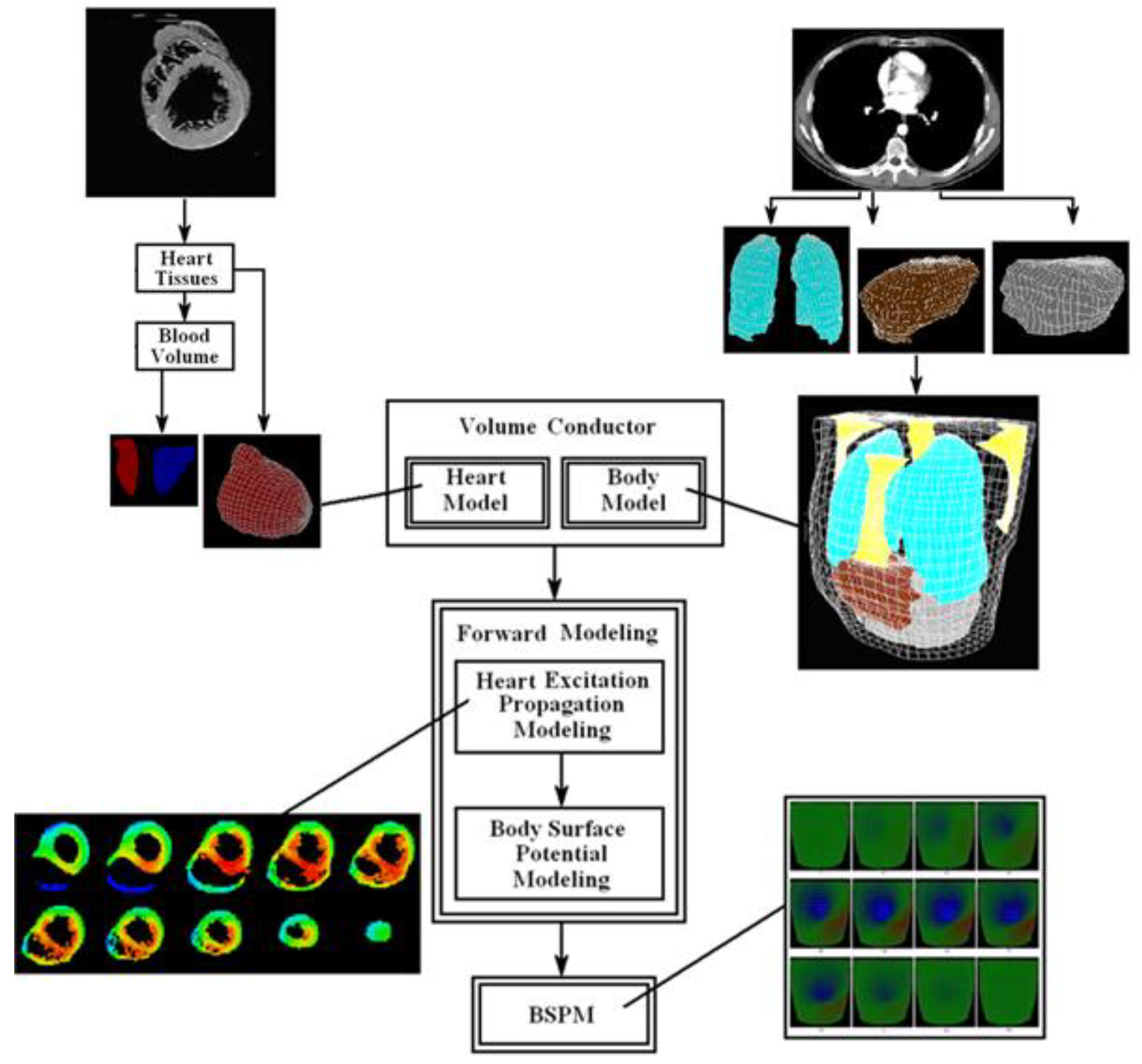
Figure 4.
CC chart of Table 1.
Figure 4.
CC chart of Table 1.
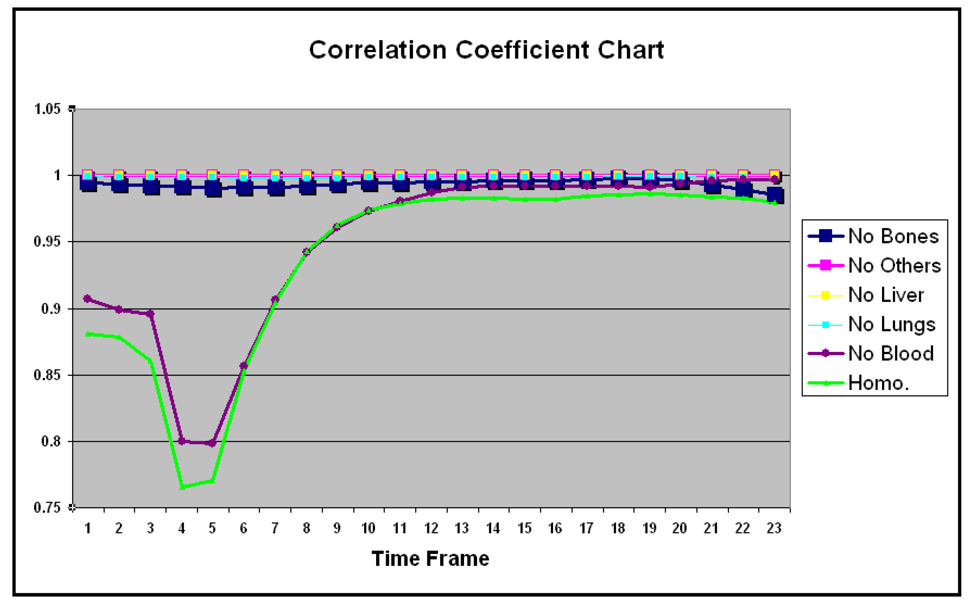
Figure 5.
RE chart of Table 2.
Figure 5.
RE chart of Table 2.
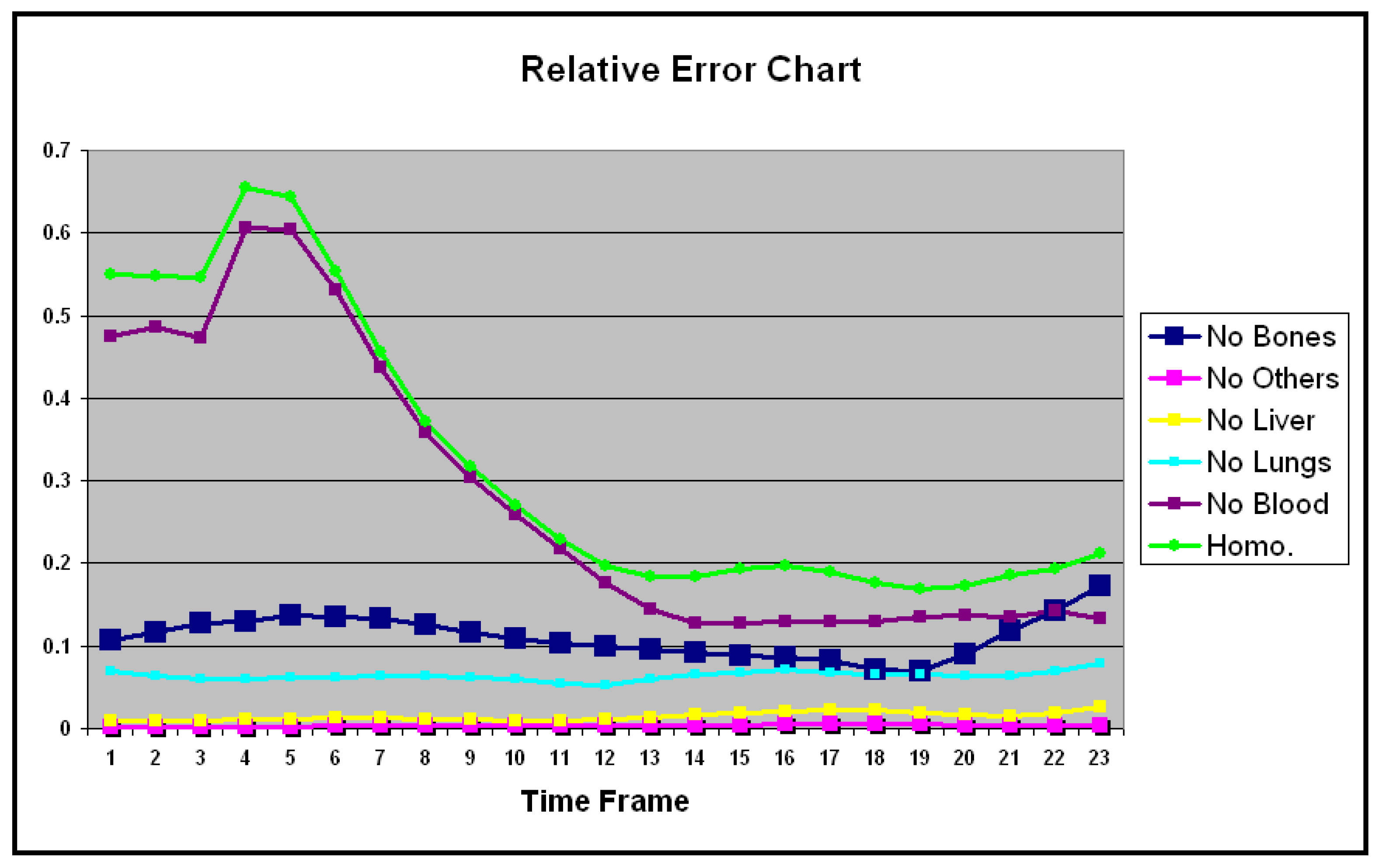
Table 2.
CC between the full inhomogeneous body and the remove of individual organ form the body.
| No Bones | No Others | No Liver | No Lungs | No Blood | Homo. | |
|---|---|---|---|---|---|---|
| 1 | 0.994 | 1.000 | 0.999 | 0.998 | 0.907 | 0.880 |
| 2 | 0.993 | 0.999 | 0.999 | 0.998 | 0.898 | 0.878 |
| 3 | 0.991 | 0.999 | 0.999 | 0.998 | 0.895 | 0.860 |
| 4 | 0.991 | 0.999 | 0.999 | 0.998 | 0.800 | 0.765 |
| 5 | 0.990 | 0.999 | 0.999 | 0.998 | 0.797 | 0.770 |
| 6 | 0.991 | 0.999 | 0.999 | 0.998 | 0.856 | 0.852 |
| 7 | 0.991 | 0.999 | 0.999 | 0.998 | 0.906 | 0.904 |
| 8 | 0.992 | 0.999 | 0.999 | 0.998 | 0.942 | 0.942 |
| 9 | 0.993 | 0.999 | 0.999 | 0.998 | 0.961 | 0.962 |
| 10 | 0.994 | 0.999 | 0.999 | 0.998 | 0.972 | 0.973 |
| 11 | 0.994 | 0.999 | 0.999 | 0.998 | 0.980 | 0.979 |
| 12 | 0.995 | 0.999 | 0.999 | 0.998 | 0.986 | 0.981 |
| 13 | 0.995 | 0.999 | 0.999 | 0.998 | 0.990 | 0.983 |
| 14 | 0.995 | 0.999 | 0.999 | 0.998 | 0.992 | 0.983 |
| 15 | 0.996 | 0.999 | 0.999 | 0.998 | 0.991 | 0.981 |
| 16 | 0.996 | 0.999 | 0.999 | 0.998 | 0.991 | 0.982 |
| 17 | 0.996 | 0.999 | 0.999 | 0.998 | 0.992 | 0.984 |
| 18 | 0.997 | 0.999 | 0.999 | 0.999 | 0.991 | 0.985 |
| 19 | 0.997 | 0.999 | 0.999 | 0.999 | 0.991 | 0.985 |
| 20 | 0.996 | 0.999 | 0.999 | 0.999 | 0.993 | 0.985 |
| 21 | 0.993 | 0.999 | 0.999 | 0.998 | 0.995 | 0.983 |
| 22 | 0.989 | 0.999 | 0.999 | 0.998 | 0.996 | 0.983 |
| 23 | 0.985 | 0.999 | 0.999 | 0.997 | 0.996 | 0.979 |
| Mean | 0.993 | 0.999 | 0.999 | 0.998 | 0.949 | 0.937 |
| SD | 0.002 | 0.000 | 0.000 | 0.000 | 0.061 | 0.068 |
Table 3.
RE between the full inhomogeneous body and the remove of individual organ form the body.
| No Bones | No Others | No Liver | No Lungs | No Blood | Homo. | |
|---|---|---|---|---|---|---|
| 1 | 0.106 | 0.001 | 0.008 | 0.069 | 0.473 | 0.549 |
| 2 | 0.117 | 0.001 | 0.009 | 0.063 | 0.485 | 0.547 |
| 3 | 0.127 | 0.001 | 0.009 | 0.060 | 0.473 | 0.546 |
| 4 | 0.129 | 0.001 | 0.010 | 0.060 | 0.606 | 0.655 |
| 5 | 0.137 | 0.002 | 0.011 | 0.061 | 0.604 | 0.643 |
| 6 | 0.134 | 0.003 | 0.012 | 0.062 | 0.532 | 0.554 |
| 7 | 0.134 | 0.003 | 0.012 | 0.063 | 0.436 | 0.455 |
| 8 | 0.125 | 0.003 | 0.012 | 0.063 | 0.357 | 0.371 |
| 9 | 0.116 | 0.003 | 0.010 | 0.061 | 0.304 | 0.317 |
| 10 | 0.108 | 0.003 | 0.009 | 0.059 | 0.259 | 0.270 |
| 11 | 0.102 | 0.003 | 0.009 | 0.053 | 0.217 | 0.228 |
| 12 | 0.100 | 0.003 | 0.010 | 0.052 | 0.176 | 0.197 |
| 13 | 0.096 | 0.004 | 0.013 | 0.059 | 0.144 | 0.184 |
| 14 | 0.091 | 0.004 | 0.016 | 0.064 | 0.128 | 0.183 |
| 15 | 0.088 | 0.004 | 0.018 | 0.068 | 0.127 | 0.193 |
| 16 | 0.086 | 0.004 | 0.021 | 0.070 | 0.130 | 0.197 |
| 17 | 0.081 | 0.005 | 0.023 | 0.068 | 0.130 | 0.189 |
| 18 | 0.071 | 0.005 | 0.023 | 0.065 | 0.129 | 0.176 |
| 19 | 0.069 | 0.004 | 0.018 | 0.065 | 0.134 | 0.168 |
| 20 | 0.089 | 0.004 | 0.015 | 0.064 | 0.136 | 0.172 |
| 21 | 0.117 | 0.003 | 0.014 | 0.063 | 0.135 | 0.185 |
| 22 | 0.142 | 0.002 | 0.017 | 0.070 | 0.141 | 0.193 |
| 23 | 0.172 | 0.003 | 0.026 | 0.079 | 0.132 | 0.211 |
| Mean | 0.110 | 0.003 | 0.014 | 0.063 | 0.278 | 0.321 |
| SD | 0.024 | 0.001 | 0.005 | 0.005 | 0.171 | 0.170 |
Disclaimer/Publisher’s Note: The statements, opinions and data contained in all publications are solely those of the individual author(s) and contributor(s) and not of MDPI and/or the editor(s). MDPI and/or the editor(s) disclaim responsibility for any injury to people or property resulting from any ideas, methods, instructions or products referred to in the content. |
© 2025 by the authors. Licensee MDPI, Basel, Switzerland. This article is an open access article distributed under the terms and conditions of the Creative Commons Attribution (CC BY) license (http://creativecommons.org/licenses/by/4.0/).
Copyright: This open access article is published under a Creative Commons CC BY 4.0 license, which permit the free download, distribution, and reuse, provided that the author and preprint are cited in any reuse.


