
Submitted:
11 July 2023
Posted:
13 July 2023
You are already at the latest version
Abstract
An estimation of the electric sources in the heart were conducted using a novel method, based on Huygens’ Principle, aiming at a direct estimation of equivalent bioelectric sources over the heart surface in real time. The main scope of this work was to establish a new, fast approach for the solution of the inverse electrocardiography problem. The study was based on recorded electrocardiograms (ECGs). Based on the Huygens’ principle, measurements obtained from a patient’s thorax surface were interpolated over the surface of the employed volume conductor model and considered as a secondary Huygens’ sources. These sources, being non-zero only over the surface under study, were employed to determine the weighting factors of the eigen-functions expansion describing the generated voltage distribution over the whole volume conductor volume. With the availability of the potential distribution stemming from measurements, the electromagnetics reciprocity theorem is applied once again to yield the equivalent sources over the pericardium. The methodology is self validated, since the surface potentials calculated from these equivalent sources are in very good agreement with ECG measurements. The ultimate aim of this effort is to create a tool providing the equivalent epicardial voltage or current sources in real time, i.e. during the ECG measurements with multiple electrodes.
Keywords:
(ECG)
; Huygens’ Principal
; reciprocity theorem
; finite element method
1. Introduction
In an increasing aging populace, a total global burden of disease has been raised [1] in the western world. The leading contributors to disease burden among the elders are cardiovascular diseases (30.3 % of the total burden in people aged 60 years and older), malignant neoplasms 15.1 % , chronic respiratory diseases 9.5 % , musculoskeletal diseases 7.5 % , and neurological and mental disorders 6.6 % [1]. A substantial and increased proportion of morbidity and mortality due to chronic disease have already observed in elderly populace. This caused an increasing demand of more accurate and non-invasive methods of diagnosis of such diseases. In addition, understanding the inner working mechanisms of the human body would be played a important role to cure and treat them. These reasons have lead to an all-increased demand of more accurate medical image techniques. The most known medical image methods include X-rays, computed tomography (CT) scan, magnetic resonance imaging (MRI), ultrasound and nuclear medicine imaging, including positron-emission tomography (PET),[2]. Lately, techniques utilizing recordings of the electric activity of different parts of a human bodies have emerged as novel medical imaging methods,[3,4]. The electroencephalography (EEG) and electrocardiography (ECG) are the most widespread electric recording techniques, which monitor the electric activity of the brain and heart, respectively.
Electric recordings of living organs are utilized as non-invasive method detecting different anomalies of the living tissues measuring the surface potentials of different part of the body. For example abnormal electric responses of different tissues (conductivity anomalies) may use to indicate damage or a failure of a system before the first symptoms displayed,[3]. These passive techniques are not demanding external electromagnetic source which can harm the human body as CT and X-Rays. Nowadays, the most used technique is the ECG to monitor the condition and detect different diseases of the heart. However, these recordings have not yet been fully understand narrowing the possibility of a successful diagnosis. Those potentials are usually represented as multiply time series of the measured area. Assuming that in a standard ECG 12 leads are utilized, it is very difficult to detect the anomaly. For this reason, there is a great research effort towards transforming the conventional electrical recordings into an equivalent 2D or 3D representation of the tissue’s electric activity. The ultimate aim of this work is the estimation of distributed equivalent voltage/current sources over the heart surface (epicardial) or the brain volume in real time. Estimating the equivalent sources permits the representation of the electric activity of heart or brain in 3D targeting the spatial detection of the different anomalies.
The potential to be able to characterize the electric activity of different organs using a non-invasive method for the computation of their surface potentials is a major breakthrough especially in real time applications (i.e. diagnosis of a cardiac arrest). Such non-invasive methods are commonly known as the inverse problem of electroencephalography and electrocardiography accordingly, which have been studied in great extent within the scientific community. Inverse problems aim at the specification of those equivalent sources responsible for the genesis of several known (measured) potential on a surface that encloses them. In the case of the inverse electrocardiography problem, the known potentials correspond to the ECG recordings of a patient and as for the equivalent source, it is the one representing the electric activity of the heart.
As referred in [5], the inverse problem’s models in the literature include: a single dipole with time-varying unknown position, orientation and magnitude; a fixed number of dipoles with fixed unknown positions and orientations but varying amplitudes; fixed known dipole positions and varying orientations and amplitudes; variable number of dipoles (i.e. a dipole at each grid point) but with a set of constraints. As regards dipole moment constraints, which may be necessary to limit the search space for meaningful dipole sources, Rodriguez-Rivera et al.[6] proposed four dipoles’ models with different dipole moment constraints. These are (i) constant unknown dipole moment; (ii) fixed known dipole moment orientation and variable moment magnitude; (iii) fixed unknown dipole moment orientation, variable moment magnitude; (iv) variable dipole moment orientation and magnitude.
The inverse problem starts with a guess for the equivalent source to be sought usually of unitary moment amplified uniform. It is widely accepted in the literature related to biomedical inverse problems [7] that when the source location is sought, the problem becomes highly non-linear and thus very difficult to solve. On the contrary, when sources with fixed location with the unknown being their amplitudes and orientation (i.e. dipoles with unknown moments , ,) are considered, then the inverse problem becomes almost linear. This claim is essentially the key hidden behind the possibility of a direct inverse problem solutions as carried out herein, without any need for iterative solutions. The effort within this work is directed to a different approach for inverse ECG problem. A distributed current source over the epicardium is sought for each temporal sampling. This approach serves the ultimate task to yield a current and voltage distribution flowing over the the cardial muscle during its temporal cycle. In this manner any damage in the cardiac muscle would be reflected to some irregularity in the epicardial current flow. We performed a direct solution for either discrete (not presented herein) and distributed sources as described next. In both cases the source origin (position) is assumed fixed but with unknown magnitude. The methodology validation proved the almost linear claim.
The first step for the solution of the inverse problem is the initial guess about the equivalent fixed location source within the thorax model. Having both the volume conductor model and the known sources, the solution of the forward problem takes place resulting to a potential distribution throughout the model (). For the inverse solution to be established, alongside the calculated potential distribution, a set of measured data needs to be acquired denoted as (). Within each iteration of the inverse problem, a cost function is established which is usually defined as the sum of the squared differences (SSQ) between the calculated and the measured potentials [8,9]. The problem is iteratively solved until its residual (SSQ) is minimized. Within every iteration the source parameters, i.e. the moments of the dipoles, are gradually altered resulting to a different solution of the forward problem which are anew compared to the measured potentials. Common search methods include iterative Kozlov- Maz’ya-Fomin (KMF) method [10], genetic algorithms [11],Newton-Raphson Method, Gauss-Newton [12], Levenberg-Marquardt algorithm [13], Tichonov relugation [14,15] and neural networks [16,17]. Nowadays, the main research effort is towards finding a more efficient regularization technique to increase the accuracy and convergence time of the above algorithms, [18,19,20,21,22,23,24]. However, a major drawback of the inverse problems that are currently under use is the high computational time and resources needed.
The method proposed within the context of this article is addressing the above-mentioned problems, i.e. the decrease of the computational time and resources needed for the estimation of the equivalent brain or heart sources. The proposed method, based on Huygens’ Principal, aims at a direct estimation of equivalent bio-electric sources. The main difference between the classical approach of the inverse problem solution and the proposed method lies on fact that the latter one does not require iterative solutions of the forward problem. Specifically, using Huygens’ principal, we can consider a closed surface (i.e. the thorax or head surface) surrounding the sources under study. Then, the potential values measured on those surfaces can be regarded as secondary Huygens’ sources which, as it can be theoretical proven, generate the same potential distribution as the primary ones. Consequently, the secondary sources have a non-zero value only on the selected closed surface while they are zero on the rest of the volume model. In more detail, we initially consider a function that generates the potentials within the volume conductor model. In order to achieve a faster and computationally efficient method, the function is handled as an eigenfunctions’ expansion. Those eigenfunctions are extracted after the numerical solution of the eigenvalues problem, which is formulated under the finite elements method (FEM). The first step towards our final goal, is to acquire a set of ECG or EEG measurement recorded from the surface of the thorax or the head accordingly. Using appropriate shape functions, we interpolate the data as to acquire a potentials surface distribution on the whole model surface. We then equate the generated surface distribution with the expansion of the function and by exploiting the orthogonality of the eigenfunctions and integrating over the thorax surface we extract the weighting factors of the expansion. Knowing the weighting factors that correspond to our volume conductor model, we can consider that function not only generates the surface potentials but also the potentials within the model, meaning that the heart surface potentials can also be estimated. Now, is the time to apply Huygens’ principle for the second time regarding the primary equivalent sources on the heart surface (epicardium). Like before, the sources are considered non-zero only on the heart surface while they equal to zero anywhere else. By integrating the heart surface and using the appropriate shape functions we estimate the epicardium potentials. An alternative approach refers to estimation of equivalent current densities flowing over the epicardium. Although this is theoretically validated herein, its explicit solution is left for future task. It is anticipated that the proposed method will enable an “epicardial source mapping” in almost real time. Namely, within a few minutes, the epicardial potential distribution could be extracted. Thus, if this is indeed possible, an important diagnostic tool could be established. Having the epicardial source distribution versus time, pathological cases can be distinguished with ease. Knowing the physiological activation timing for the heart, malfunctions of cardiac components, or even region with no activation (i.e. necrosis), could be determined.
2. Materials and Methods
2.1. Volume Conductor Problem
For the solution of the studied biomedical cases, and any other problem in general, a proper model must be employed as for the numerical solution to take place. Within the context of this article, the geometry the thorax will be studied. The human body has a particularly complicated internal structure as it is comprised of several different types of tissues that introduce a high inhomogeneity and must all be considered for the construction of a realistic volume conductor model. As expected, the higher the accuracy of the model, the higher the accuracy of the numerical method will be. Alongside the accuracy, however, the model is also closely correlated to the execution time of the algorithm. Thus, a trade-off between those two parameters must be consider as to result to models that could be employed in real-time scenarios.
When talking about volume conductor models, we refer to discretization schemes that transform the continuous geometry to finite number of elements that are homogenous as units. The volume conductor model employed for the purposes of this article was in the context of the Finite Element Method (FEM). One of the main advantages of the FEM method is that through the utilization of arbitrary shaped elements (i.e. tetrahedrons, hexahedrons etc.) it can describe almost any arbitrary given geometry. Depending on the problem, each element is characterized by properties that are related to the physical model, i.e. the conductivity or permittivity of the tissues. The volume conductor models used were taken from the classical related articles of Jorgenson [25], Gabriel [26] and the data base of ITIS [27] but in the form adapted from [28].
The thorax model comprises of 32 levels, or 33 section, [28]. The vertical distance between the sections is constant and equals to (). Horizontally, and by average, the elements are of about varying from to . In total, the model consists of 9729 nodes which assemble 8800 general hexahedrons. Figure 1a illustrates a human thorax alongside the corresponding sections employed for the composition of the model, with the numbering on the left being the original one [29] and on the right the one employed herein.
The assembly of the thorax model, i.e. placing the sections above each other, yield the exploitation of a reference axis. This axis was located outside the model as to not interfere with any of the sections. The distance between each section and the reference axis was not constant but was defined after considering the shape of the spine. The above analysis resulted to the volume conductor model of Figure 1c, where the heart elements are highlighted. Elements consisting of more than one tissues are denoted with a combination of the corresponding letters. The conductivity of such element is calculated as:
where the volume of tissue-n, the corresponding conductivity and the volume of the element.
The electric dipole, employed for the source representation, consists of two equal and opposite electric charges () whose distance is l, Figure 2a. The electric dipole moment is then defined as , where the vector’s orientation is defined from the negative to the positive charge. The elementary dipole was employed assuming infinitesimal distance l, as presented in Figure 2b. The main advantages of this dipole source configuration are the following:
- Due to its small size, it is always entirely located within a single discrete element,
- It behaves as an impulse function; thus, it excites both higher and lower order harmonics,
- It has the greatest possible degrees of freedom.
An equivalent geometry-structure (Figure 2c) for the source can replace the dipole where currents equivalent are applied upon the nodes of the element including the dipole, a configuration introduced by Kassem A. Awada et al [30]. Thus, for each unknown dipole moment the problem transforms into a form were the node values of the excitation currents through are sought. If a node belongs to an element where a dipole is present, then the current can be calculated as [30]:
where the basis or shape function corresponding to node i. If the node under study does not belong to an element containing a dipole then the equals to 0. Equation (2), considering its discrete form, yields:
where () are local domain coordinates of the isoparametric transformation [31].
2.2. Direct Inverse Problem Solution
In the proposed method, the term inverse does not describe an iterative solution of the forward problem, as it usually does, but it rather implies the direct extraction of an equivalent internal current density or voltage source distribution given a set of surface potential measurements. The methodology that follows, is the basis for the proposed direct solution of the inverse problem. The methodology is organised in a step-by-step approach as:
- Interpolation of the discrete electrode voltages to generate equivalent surface potential source distribution.
- Consider an eigenfunction expansion for the volume potential distribution and estimate its weighing factors by equating it to the source distribution (of step 1) by exploiting the eigenfunction orthogonality.
- Assume a source distribution over the epicardium (or inside the brain) as an expansion of FEM basis functions. Its weighing factors are estimated by equating to the volume potential and exploiting the FEM basis function’s orthogonality.
- The resulting internal sources are validated by comparing their generated potential to the original ECG or EEG measurements.
Let be the function that generates the potentials within and upon the thorax given a specified excitation and , with , the M measurements recorded from the thorax surface. Those surface potentials are regarded as a secondary Huygens surface source.
The equivalence principle was introduced by A. E. Schelkunoff in 1936 [32] and forms a more strict statement of Huygens’ principal, which namely states that “each point of a wave front can be considered as the source of secondary wavelets that spread out in all directions with a speed equal to the speed of propagation of the waves [33]”.
Given a source g and a surface S that encloses it, there is a certain source h distributed over the surface S that gives the same field outside (or inside) this surface. Thus, two source distributions that produce the same field within a region are said to be equivalent within that region. Consequently, when we are interested in the field of a specific region, prior knowledge of the actual sources is not needed as long as the equivalent sources can be sought.
Let’s assume, for instance, and an electric and a magnetic source respectively located within the volume V1 and generating the fields and as it can be seen in Figure 3a. An equivalent problem to this could be the one presented in Figure 3b, where the internal sources have been removed and replaced by their equivalent surface sources and that generate the internal field, while the external field can be considered as null (Love’s Equivalence Principles). Namely, those equivalent surface sources are [34]:
In terms of the problem under study, g corresponds to the sought equivalent heart (or brain) activity, S to the thorax or scalp surface and the auxiliary Huygens sources (h) can be extracted from the recorded surface potentials through interpolation (Figure 3c). As mentioned above, the surface distributed source w can produce the same field either inside or outside the enclosing surface S. We Consider the case of electrostatic sources and electric fields, i.e. and , when the external field is considered null. Field equivalence principle has been exemplified for various different cases by Branko Popovich in his classic work [35]. Therein, the present case of the static or quasi-static problem is also analyzed. This distributed source can be either a current or a potential source. The problem formulation for both cases follows.
2.2.1. Step-1: Surface source distribution
The equivalent surface sources are estimated from the measured potential (ECG or EEG) as:
Where the applied surface source, the original one, the originally generated electric field and the voltage. In our case, corresponds to the measured potential over the surface of the model, i.e. . However, to address Huygens’ Principle distributed surface sources must be employed.
Explicitly, due to the fact that not all surface thorax nodes can be corresponded to a specific electrode, there are nodes for which there is no available measurements’ information. Thus, to address this problem the provided recorded potentials must be interpolated to result a "measured" surface potential distribution that cover all nodes as seen in Figure 4.
A pyramid element interpolation of the provided voltage data was implemented to calculate the surface potential of the thorax/head,[36]. Let’s consider the pyramid element of Figure 5. In Figure 5, the purple circles suggest nodes for which the value is considered known, i.e. the potential measurement from the corresponding electrode, whereas the black ones denote nodes for which no information is available. In the problem under study, the electrodes are evenly placed throughout the thorax, having an electrode placed every third level with a spacing of one node between every two electrodes of the same level, as it can be seen in Figure 1c and Figure 5. To enable the calculation of the potential distribution, all pyramids were centred around nodes for which the potential was known. Thus, for the evaluation of each node, all the contributions of its surrounding electrodes must be taken into account. Roughly speaking, considering the interpolation shape function for the pyramid , the potential for a specific node can be calculated as:
where with N being the number of the pyramid nodes and are the measured potentials for all the neighbour nodes that are associated to a specific electrode. The pyramid shape function was defined for a reference element with corners (Figure 5). The basis (shape) function for pyramids is not unique, thus within the context of this dissertation the formulation presented in [36] was adapted, which approached the pyramid formulation as the composition of two tetrahedral and .
The above procedure yields the potentials at all the surface nodes. However, the basic Huygen’s principle asks for a continuous surface source distribution. This was obtained exploiting the FEM interpolation-shape functions, within every quadrilateral surface element as:
2.2.2. Step-2: Volume Potential eigenfunction expansion
Let be the distributed current source over the surface of the model and the generated potential throughout the volume conductor model. Therefore, the overall system can be described as:
Where is the Laplacian operator. The volume potential can be described as a modal eigenfunction expansion:
The procedure of our previous work [8] is adopted to estimate the weighing factors . Every pair of eigenvalue and eigenvector follows the property:
where are the eigenvectors of the Laplacian operator and their corresponding eigenvalues. Equation (12) is multiplied by the weighing factors and integrated over the whole domain volume as:
Although, Equation (13) establishes a relation with the distributed current source this is a type of summation. In order to isolate the weighing factors this is multiplied by another eigenfunction before integration to yield:
The source is restricted only on the surface while is zero outside that, thus the right-hand side integral is reduced into a surface one. Since the eigenfunction and obey the orthogonality property (third side of (14)) thus the weighing factor is isolated as;
Equation (15) provides the volume potential distribution when a surface current is extracted as in the previous Section 2.2.1. Alternativly, these can be estimated directly from the surface voltage as follows. Considering a distributed voltage source over the outer surface of the model, we can assume that this is a subset of the function generating the voltage throughout the model volume, i.e. , thus:
Herein, the voltage source is thought to be the voltage measurements recorded from the surface of the thorax or head. However, the electrodes employed for the measurements () acquisition may be limited to only a few on the surface model’s nodes (Figure 4a). In this usual case, an interpolation of the data should precede as to extract the desired potential distribution over the outside surface (). This potential source distribution is non-zero only on the surface of the model while vanishes anywhere else (Figure 4b). For the weighting factors to be calculated, the orthogonality of the eigenvectors is again exploited. Thus multiplying (16) by an eigenvector and exploiting the orthogonality property, yields to:
Then:
Nevertheless, keeping in mind Huygens’ Principle the above integral degenerates to a surface one as the sources have values over the model surface and equal to zero elsewhere. Thus, Equation (18) reduces to:
2.2.3. Step-3:Estimate the internal Equivalent Sources
Knowing the weighting factors, we can now consider that the same function generates the potential distribution over the epicardium surface . The sought continuous epicardium voltage source is discretized by the aid of a finite element mesh as an expansion of the nodal voltage values.
where the FEM interpolation shape function over the heart surface and the voltage on the surface of epicardium. These epicardium voltages are assumed identical to the corresponding volume potentials obtained in step-2, as.
Given the shape functions and their orthogonality properties, the following applies:
where is 1 if the shape functions are normalized, otherwise is a normalization factor (). In turn Equation (21) yields:
Summarizing, and in order to extract the epicardial potential distribution, the following 6 steps can be generally identified:
- Acquisition of a data set corresponding to measurements recorded from the surface of the thorax.
- Interpolation of the acquired recordings throughout the surface of the model, i.e. the thorax.
- Calculation of the weighting factors exploiting the Equations (15) or (19) depending of the selected source type.
- Adaptation of the problem as to describe the heart surface (Huygens’ Principle) and selection of the appropriate shape functions as for them to comprise an orthogonal basis.
- Exploitation of the orthogonality over the heart and integration over the epicardium.
- Extraction of the epicardium potentials using Equation (19).
2.3. Numerical Implementation
Within the context of this paragraph the numerical results of the employed method will be obtained. The proposed method starts by the acquisition of a set of measured data. The measured data employed for the solution of the proposed method is the same as in the case of the inverse ECG problem, i.e. recordings of a 198-electrodes vest obtained from Utah University, [37].
Herein, the voltage source is thought to be the voltage measurements recorded from the surface of the thorax. This potential source distribution is non-zero only on the surface of the model while zero anywhere else. Having the potential distribution throughout the thorax calculated, alongside the eigenvectors resulted from the eigenanalysis of the conductivity matrix Y, we can address our main objective. Thus, the weighting factors for each time internal can be extracted. As clearly suggested from (14), for the resulting weighting factors the integration of the product over the thorax surface must be evaluated. An obvious solution to the problem would be the exploitation of Gauss integration through FEM over the corresponding quadrilaterals assembling the model’s surface. Such an approach, however, and considering that the potential distribution refers to multiple time instances (consisting of namely 750 samples for each of the 128 selected electrodes), introduces an unacceptable computational burden alienating us further from a fast solution of the inverse problem. Thus, to avoid this problem the integral of Equation (19) was approximated from a different point of view. Let’s consider two functions and for which the following integral, with regard to Equation (18) is sought:
where the subscript i of function denotes the time interval, as is time dependant contrary to . In our case, can be replaced with the extracted eigenvectors of the model while stands in for the measured potential of the surface model’s nodes. Namely, we have:
- , which is an array containing the m eigenvectors for each of the n nodes and
- , which is an array consisting of the n nodes of the model from which non-zero are only the ones corresponding to the surface of the thorax, and the different time instances t.
The main objective is to associate the integral to the time invariant functions, i.e. the eigenvectors, as for it to be calculated only once. This is an indeed possible approximation as the time varying function, i.e. the potential distribution, presents slight alterations between neighbourly nodes, thus it can be considered as constant for a given quadrilateral for a time instance. The integral of the time-invariant function can be regarded as a geometrical factor that encapsulate all the information related to the geometry of the model’s surface.
The utilized approach is based on the exploitation of the isoparametric transformation employed in the context of FEM. As described above, considering the potential distribution constant over a quadrilateral for a time instance i, only the integral of the eigenvectors over the element needs to be evaluated. Namely,
where the N is the total number of samples, 750 in current case. Denoting as the result of the integration, obtained through FEM, that inherently contains the information about the model’s geometry and the samples of the potential distribution, Equation (23) can be expressed into its discrete form:
Considering the extracted weighting factor, the epicardium potential distribution can now be calculated by exploiting utilizing Equation (25).
3. Numerical Results
The solution starts with the acquisition of an ECG potential distribution recorded from an adult’s thorax [37], which in our case was a healthy male. Given the net of electrodes employed during the recordings, the first step is to associate the electrode position with our volume conductor model’s node, i.e. the thorax model. This association is, of course, an approximation and therefore some errors are introduced to our computations. To avoid additional errors, not all recording electrodes were considered but only the 128, out of the 198 (12 levels x 16 electrodes), were used. Out of the 12 levels of electrodes in the original distribution, only the first 8 were selected, as it can be seen in Figure 1. Those four levels were corresponded to the upper chest and were left out as to minimize possible errors due to the shoulders of our original model.
The inverse ECG problem starts with the solution of the system of Equation (10), as described in Section 2.2.2. The first 200 eigenvalues are presented Figure 6 along with some eigenvectors at the 20th cross-section of thorax model as depicted in Figure 1. For the evaluation of the problem however, is of crucial importance to inspect the eigenvalue distribution before we try to solving the Equation (15) or (19). As clearly presented in Figure 6a, the values of the first few eigenvalues are very small regarding the first ones. Note that the very small eigenvalues are usually highly inaccurate and if included the may cause instability or large errors in the expansion. Consequently, without affecting the accuracy of the calculated solution, it is possible to discard those very small eigenvalues as to achieve better stability and faster forward solution. The difficult related to this approach is that herein and in electromagnetic in general the useful information lies in the small low order eigenvalues. Hence, the challenge is to discard only some very small eigenvalues which represent eigenvectors with dominant numerical "noise"-inaccuracies. On the other end we may discard, some very large eigenvalues (high order) which do not include useful information. Since eigenvalues constitute the spectral representation of the structure, then Parseval’s theorem applies. Namely, the square of the weighing factors represent the power carried by that eigenmode. Considering the eigenvalues contributing to the of the total energy, 9589 eigenvalues out of 9729 are retained. Even though this might seem a small reduction of the matrix rank, considering volume conductor models of higher discretization the above-mentioned technique can result to an important decrease of the computational time without affecting the results’ accuracy. But most important it highly improves the system matrix condition number significantly improving the expansion accuracy, namely the condition number is decreased from to . It is important to state that even after the rejection of just the first eigenvalue, the condition number decreases to which suggest that the problem lies within the first few eigenvalues.
In order to interpret the results, it is necessary to denote all the heart components involved in the cardiac activation. In Figure 7, the calculated potential distribution, as resulted from the direct inverse problem, for several time instances is presented. The calculated potential distribution over the epicardium tends to closely resemble the electric physiology of the heart. Namely, starting at about 5 msec (with the signal origin being the 1 msec) the area around SA nodes, alongside with some atrial nodes, is activated (10 ms) as in Figure 7a. Some time instances later, i.e. Figure 7b at t= 30 msec, the amplitude of the activation increases. The next nodes activated, around t= 130 msec, is the ones corresponding to the AV node, the Bundle of His and the bundle branches (Figure 7c), following the anticipated cardiac activation. After this, the ventricular depolarization taking place around 170 msec (Figure 7d), with the right ventricle activation slightly preceding. After a while, i.e. around 200 msec (Figure 7e), the left ventricle depolarizes as well. At about 500 msec, the ventricular starting their repolarization and all cells return to their resting potentials (Figure 7f).
Considering an electrocardiogram of a healthy man, the above comply sufficiently with the physiological heart activation sequencing. Namely, the cardiac activation signal starts from the SA nodes, propagates through the atrial and through the AV node, the bundle of His, the bundle branches and the Purkinje fibres is transmitted to the ventricle. The main differences between the calculated results and the physiological heart activation are observed during the atrial depolarization, which in our case is not spread throughout the corresponding atrial nodes but are rather gathered around two distinct areas (Figure 7a,b). In addition to this, AV node, the bundle of His and the bundle branches tend to be activated almost simultaneously (Figure 7c), whereas their physiological activation present a delay of several msec.
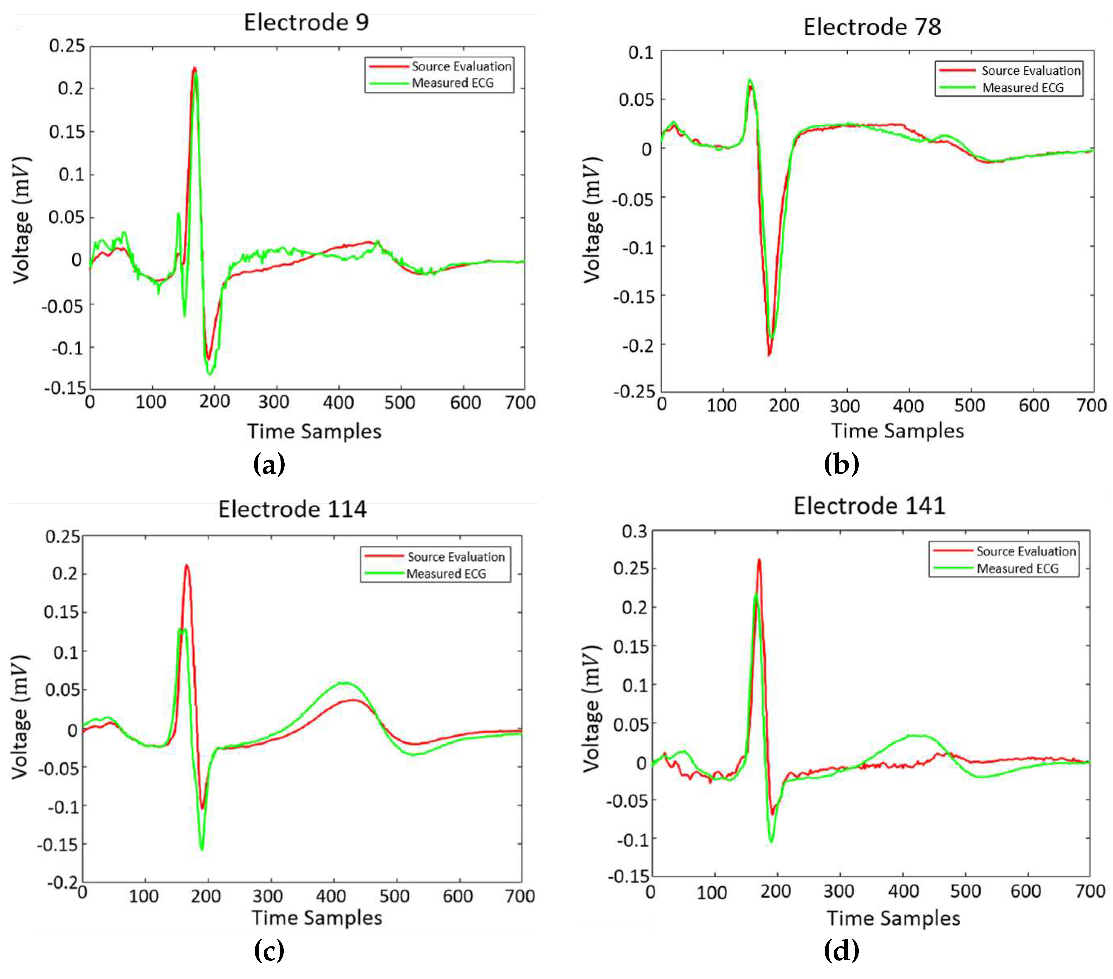
Having the epicardium potential distribution (reconstructed sources), it is now possible to determine whether the extracted equivalent source can generate the anticipated potential distribution over the thorax. These are compared against the original ECG measurements for validation purposes. Figure 8 illustrate the generated potential upon the corresponding electrodes after the evaluation of the classical forward problem, given the resulted epicardial potentials. The extracted results are given alongside the original ECG measurements. Figure 8 corresponds to electrodes 9, 78, 114 and 141 that are located on the back, on the chest, on the right and on the left side of the thorax’s patient, correspondingly. The calculated results tend to have a better behaviour when the back of the torso and the chest is concerned, whereas the results regarding the sides of the torso are sometimes unable to follow the original signal sufficiently (i.e. Figure 8c). The approach seem to approximate sufficiently the original data, even though there are electrodes where some inaccuracies are present.
It is obvious that the behaviour of the equivalent source closely resembles the physiological heart excitation. Thus, the direct solution of the inverse problem is feasible through the proposed method within only 2 minutes, whereas in the case of the classical inverse problem solution the execution time could even exceed the 2 hours. The locations of the presented electrodes over the thorax model can be found in Figure 1c. At electrodes where the calculated results closely follow the original data, i.e. Figure 8a, the percentage of their divergence is below . There are however cases where this percentages highly increases, as it is obvious in Figure 8d. In general, this percentage varies between 5-15%.
The most important outcome of the obtained epicardial source distribution is the prospect for an “epicardial source mapping”. Namely, if it is possible to map the epicardial sources versus time, then an important diagnostic tool could be established. The prospect is that for a physiological cardiac operation, the whole epicardial surface will be activated accordingly to the proper timing. On the contrary, pathological heart functioning may result in either wrong timing in the activation of the heart components or no activation at all (ex. partial necrosis). Hence, the proposed methodology, can be exploited as an advanced diagnosis tool which in a very fast and convenient way takes into account ECG (or EEG) measurements over the entire thorax (or scalp) surface.
4. Discussion and Conclusions
The main scope of this work was to establish a new, fast approach for the solution of the inverse electrocardiography problem. Based on the Huygens’ principle, measurements obtained from a patient’s thorax surface were interpolated over the surface of the employed volume conductor model and considered as a secondary Huygens’ source. This source, being non-zero only over the surface under study, was employed to determine the weighting factors of the eigenfunctions expansion describing the generated voltage distribution over the whole volume conductor volume, including the heart. For the accurate determination of the epicardial potential distribution, an integration over both the thorax and the heart surface is needed. The extracted results not only estimated sufficiently the heart potential distribution, but were also obtained within about 2 minutes, decreasing the execution time remarkably regarding the classical inverse problem formulation where several hours were needed for the solution of the problem. Having the ability to accurately extract the potential distribution over the epicardium within such a small amount of time, a significant diagnostic tool can be established enabling the epicardial source mapping. Namely, given the normal heart activation timing, different pathological heart condition can be distinguished by observing possible alteration in the activation timing or even no activation at all (i.e. partial necrosis).
5. Future Extensions
The measured methodology may be extended torward several directions within the ultimate task to achieve a real time inverse problem solution. The first priority is to solve the ECG inverse problem for the current density sources following the exact reciprocity principles as in [35]. This is expected to improve accuracy but also to more accurately reflect the epicardial electrical functioning through the current density flow. The second priority is to improve the volume conductor model of Figure 1 primaly by increasing the surface mesh density, in order to allow all measuring electrodes to be mapped on the model. This will allow the exploiting of all available measurements. The third priority is to improve the algorithm speed through employing state-of-the-art linear algebra techniques. Finally, the resulting direct inverse problem solutions will be applied to electroencephalography i.e. to estimate equivalent sources for epileptic regions or to study the activated brain areas during challenging phenomena as the brain default mode.
Author Contributions
“Conceptualization, G.K.; methodology, G.T.; software, G.T.; validation; formal analysis, G.T.; investigation, G.T.; resources, D.A.; data curation, D.A.; writing—original draft preparation, D.A.,S.K.; writing—review and editing, D.A.,G.K. and I.N.; visualization, D.A.,I.N.; supervision, G.K., G.S.. All authors have read and agreed to the published version of the manuscript.”, please turn to the CRediT taxonomy for the term explanation. Authorship must be limited to those who have contributed substantially to the work reported.
Funding
We acknowledge the support of this work by the project “Study, Design, Development and Implementation of a Holistic System for Upgrading the Quality of Life and Activity of the Elderly” (MIS 5047294), which is implemented under the Action “Support for Regional Excellence”, funded by the Operational Programme “Competitiveness, Entrepreneurship and Innovation” (NSRF 2014–2020) and co-financed by Greece and the European Union (European Regional Development Fund).
References
- Prince, M.J.; Wu, F.; Guo, Y.; Gutierrez Robledo, L.M.; O’Donnell, M.; Sullivan, R.; Yusuf, S. The burden of disease in older people and implications for health policy and practice. The Lancet 2015, 385, 549–562. [CrossRef]
- Mikla, V.I.; Mikla, V.V., Eds. Medical Imaging Technology; 2014; pp. i–iii. [CrossRef]
- Pascual-Marqui, R.D. Review of methods for solving the EEG inverse problem. 1999.
- Ak, A.; Topuz, V.; Midi, I. Motor imagery EEG signal classification using image processing technique over GoogLeNet deep learning algorithm for controlling the robot manipulator. Biomedical Signal Processing and Control 2022, 72, 103295. [CrossRef]
- Grech, R.; Cassar, T.; Muscat, J.; Camilleri, K.P.; Fabri, S.G.; Zervakis, M.; Xanthopoulos, P.; Sakkalis, V.; Vanrumste, B. Review on solving the inverse problem in EEG source analysis. Journal of NeuroEngineering and Rehabilitation 2008, 5. [CrossRef]
- Rodriguez-Rivera, A.; Van Veen, B.; Wakai, R. Statistical performance analysis of signal variance-based dipole models for MEG/EEG source localization and detection. IEEE Transactions on Biomedical Engineering 2003, 50, 137–149. [CrossRef]
- Michel, C.M.; Murray, M.M. Towards the utilization of EEG as a brain imaging tool. NeuroImage 2012, 61, 371–385. NEUROIMAGING: THEN, NOW AND THE FUTURE. [CrossRef]
- Aitidis, I.; Kyriacou, G.; Sahalos, J. Exploiting Proper Orthogonal Decomposition for the solution of forward and inverse ECG and EEG related biomedical problems. 2014, pp. 526–529. [CrossRef]
- Shou, G.; Xia, L.; Jiang, M. Solving the Electrocardiography Inverse Problem by Using an Optimal Algorithm Based on the Total Least Squares Theory. Third International Conference on Natural Computation (ICNC 2007), 2007, Vol. 5, pp. 115–119. [CrossRef]
- Zemzemi, N.; Bourenane, H.; Cochet, H. An Iterative method for solving the inverse problem in Electrocardiography imaging: From body surface to heart potential. IEEE Computers in Cardiology; MIT, , 2014.
- Jiang, M.; Xia, L.; Shou, G. The Use of Genetic Algorithms for Solving the Inverse Problem of Electrocardiography. 2006 International Conference of the IEEE Engineering in Medicine and Biology Society, 2006, pp. 3907–3910. [CrossRef]
- Chari, M.; Salon, S., Eds. Numerical Methods in Electromagnetism; Electromagnetism, Academic Press: San Diego, 2000. [CrossRef]
- Moré, J.J. The Levenberg-Marquardt algorithm: Implementation and theory. Numerical Analysis; Watson, G.A., Ed.; Springer Berlin Heidelberg: Berlin, Heidelberg, 1978; pp. 105–116.
- Kalinin, A.; Potyagaylo, D.; Kalinin, V. Solving the Inverse Problem of Electrocardiography on the Endocardium Using a Single Layer Source. Frontiers in Physiology 2019, 10. [CrossRef]
- Milan Horáček, B.; Clements, J.C. The inverse problem of electrocardiography: A solution in terms of single- and double-layer sources on the epicardial surface. Mathematical Biosciences 1997, 144, 119–154. [CrossRef]
- Zemzemi, N.; Dubois, R.; Coudière, Y.; Bernus, O.; Haïssaguerre, M. A Machine Learning Technique Regularization of the Inverse Problem in Cardiac Electrophysiology. CinC - Computing in Cardiology Conference; Laguna, P., Ed.; IEEE: Zaragoza, Spain, 2013; pp. 285–312.
- Chen, K.W.; Bear, L.; Lin, C.W. Solving Inverse Electrocardiographic Mapping Using Machine Learning and Deep Learning Frameworks. Sensors 2022, 22. [CrossRef]
- Nakamura, H.; Aoki, T.; Tanaka, H. Regularization methods for inverse problem of body surface potential mapping. Proceedings of the 19th Annual International Conference of the IEEE Engineering in Medicine and Biology Society. ’Magnificent Milestones and Emerging Opportunities in Medical Engineering’ (Cat. No.97CH36136), 1997, Vol. 1, pp. 344–347 vol.1. [CrossRef]
- Velipasaoglu, E.; Sun, H.; Zhang, F.; Berrier, K.; Khoury, D. Spatial regularization of the electrocardiographic inverse problem and its application to endocardial mapping. IEEE Transactions on Biomedical Engineering 2000, 47, 327–337. [CrossRef]
- Shou, G.; Jiang, M.; Xia, L.; Wei, Q.; Liu, F.; Crozier, S. A comparison of different choices for the regularization parameter in inverse electrocardiography models. 2006 International Conference of the IEEE Engineering in Medicine and Biology Society, 2006, pp. 3903–3906. [CrossRef]
- Shou, G.; Xia, L.; Jiang, M.; Wei, Q.; Liu, F.; Crozier, S. Truncated Total Least Squares: A New Regularization Method for the Solution of ECG Inverse Problems. IEEE Transactions on Biomedical Engineering 2008, 55, 1327–1335. [CrossRef]
- Potyagaylo, D.; Schulze, W.H.W.; Doessel, O. A new method for choosing the regularization parameter in the transmembrane potential based inverse problem of ECG. 2012 Computing in Cardiology, 2012, pp. 29–32.
- Ding, B.; Chen, R.; Wu, J. Multiscale-Wavelet Regularization Method for the Inverse Problem of Electrocardiography. 2019 International Conference on Medical Imaging Physics and Engineering (ICMIPE), 2019, pp. 1–4. [CrossRef]
- Kupriyanova, Y.A.; Zhikhareva, G.V.; Mishenina, T.B.; Bobrovskaya, A.I.; Andreev, I.V. Selection of the Regularization Coefficient in Solving the Inverse Problem of Electrocardiography by High-Frequency Low Amplitude Components of ECG Signals. 2022 International Conference on Information, Control, and Communication Technologies (ICCT), 2022, pp. 1–4. [CrossRef]
- Jorgenson, D.; Haynor, D.; Bardy, G.; Kim, Y. Computational studies of transthoracic and transvenous defibrillation in a detailed 3-D human thorax model. IEEE Transactions on Biomedical Engineering 1995, 42, 172–184. [CrossRef]
- Gabriel, C.; Gabriel, S. Compilation of the Dielectric Properties of Body Tissues at RF and Microwave Frequencies.; Internet document; available URL:http://safeemf.iroe.fi.cnr.it.
- PA, H.; F, D.G.; C, B.; E, N.; B, L.; MC, G.; D, P.; A, K.; N, K. ITIS Database for thermal and electromagnetic parameters of biological tissues, 2022. [CrossRef]
- Xanthis, C.; Bonovas, P.; Kyriacou, G. Inverse Problem of ECG for Different Equivalent Cardiac Sources. Piers Online 2007, 3, 1222–1227. [CrossRef]
- Eycleshymer, A.C.; Shoemaker, D.M. A Cross-Section Anatomy; Appleton Century Crofts, 1911.
- Awada, K.; Jackson, D.; Williams, J.; Wilton, D.; Baumann, S.; Papanicolaou, A. Computational aspects of finite element modeling in EEG source localization. IEEE Transactions on Biomedical Engineering 1997, 44, 736–752. [CrossRef]
- Theodosiadou, G.; Aitidis, I.; Terzoudi, A.; Piperidou, H.; Kyriacou, G. Discrimination of ischemic and hemorrhagic acute strokes based on equivalent brain dipole estimated by inverse EEG. Biomedical Physics & Engineering Express 2017, 3, 014001. [CrossRef]
- Schelkunoff, S.A. Some equivalence theorems of electromagnetics and their application to radiation problems. The Bell System Technical Journal 1936, 15, 92–112. [CrossRef]
- Collin, R.; Zucker, F. Antenna Theory, Part 1.; McGraw-Hill, 1969.
- Balanis, C.A. Antenna Theory: Analysis and Design; JOHN WILEY & SONS,Hoboken, New Jersey ,2005.
- Popovic, B. Electromagnetic field theorems. IEE Proc, 1981, Vol. 128, pp. 47–63.
- Wieners, C. Conforming discretizations on tetrahedrons, pyramids, prism and hexahedrons; 1997.
- University of Utah. http://www.sci.utah.edu/~macleod/bioen/be6000/labnotes/ecg/data/, Online.
Figure 1.
(a) Vertical view of human torso where the basic organs are presented alongside the horizontal sections of the anatomic atlas [29]. The numbering on the left correspond to the original sections whereas on the right is the employed numbering for the model.(b) Side view of the spine where the reference axis and the model’s sections are also illustrated.(c) Discretized thorax model for FEM simulation where the cardiac elements and electrodes position are also illustrated, the red dots are the electrodes (78,114 and 141) in front (thorax) and the blue dot the electrode 9 in the back.
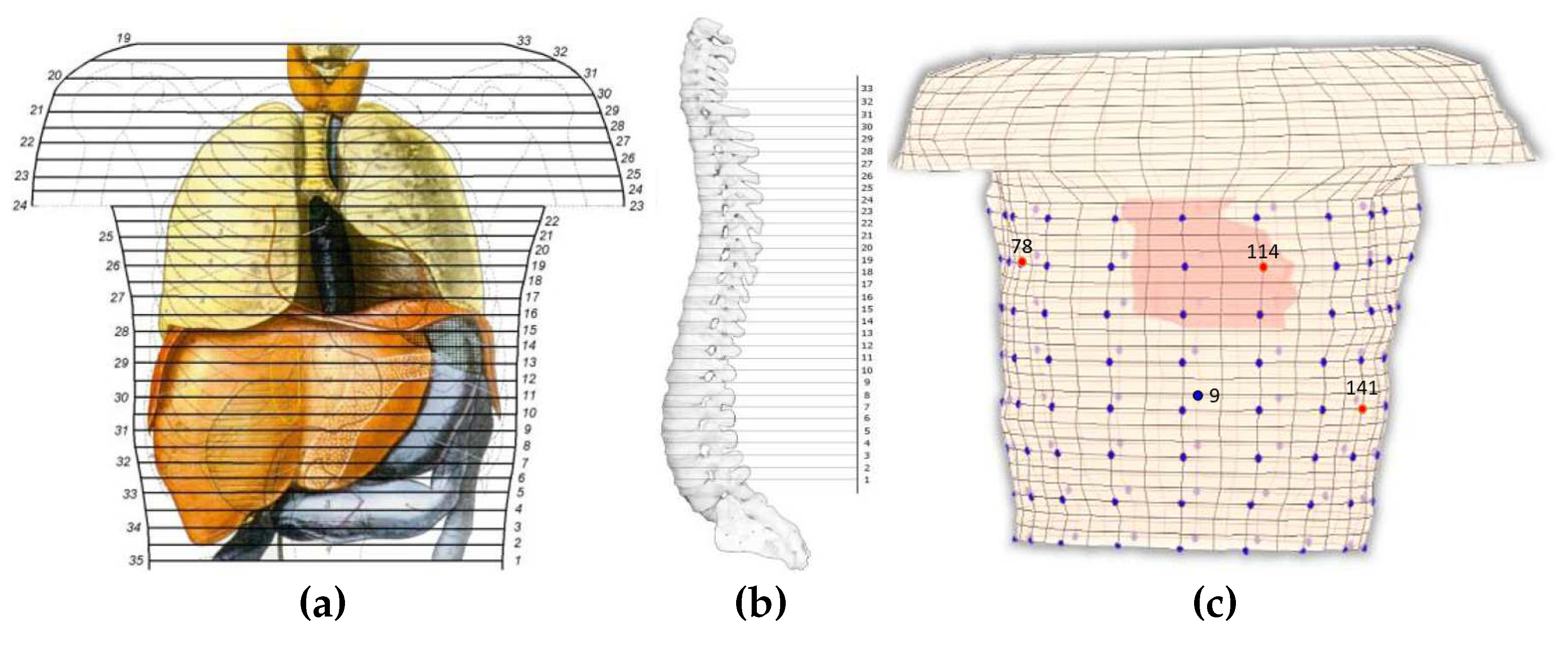
Figure 2.
Illustration of (a) a dipole located between two nodes, (b) an elementary dipole lying within a single element and (c) equivalent representation of the elementary dipole where current are applied on the nodes of the element including it.
Figure 2.
Illustration of (a) a dipole located between two nodes, (b) an elementary dipole lying within a single element and (c) equivalent representation of the elementary dipole where current are applied on the nodes of the element including it.
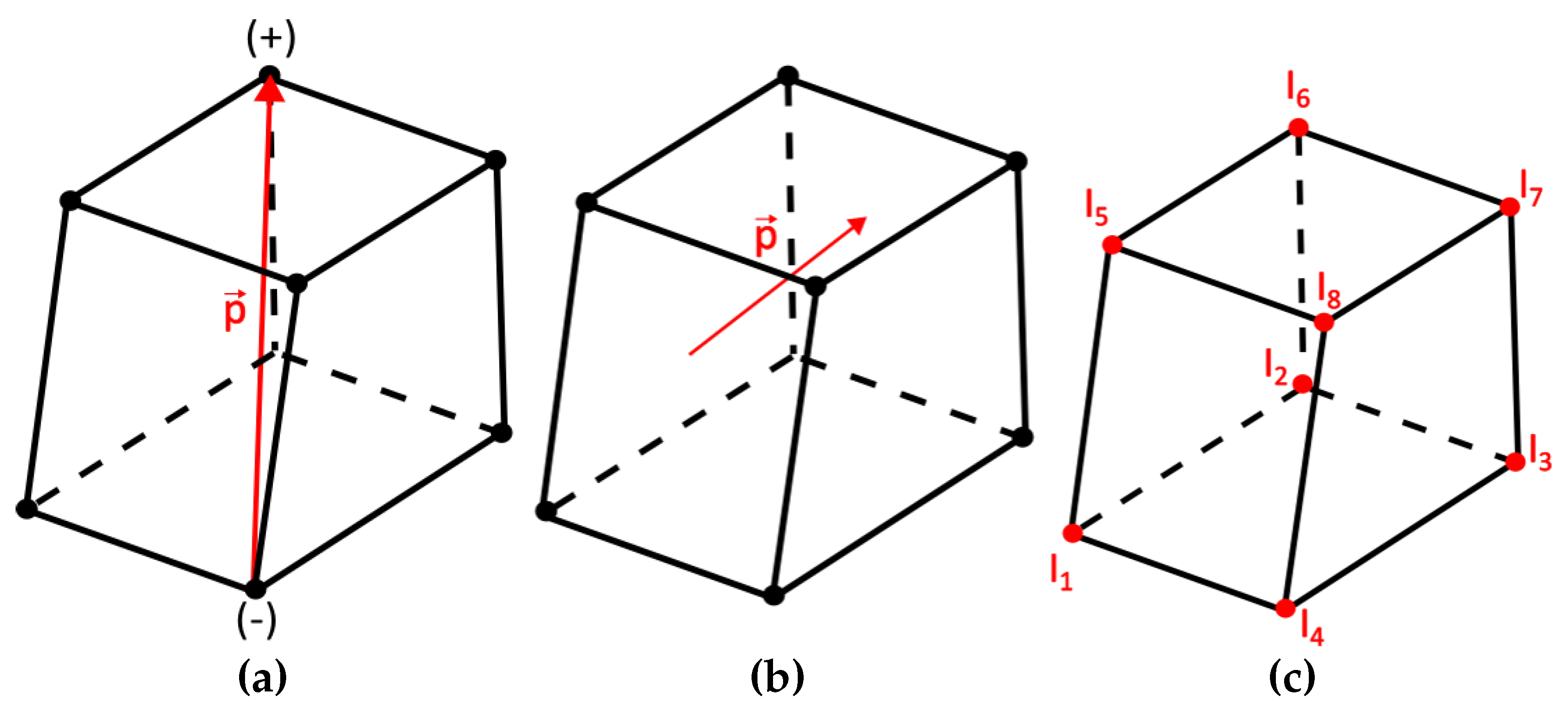
Figure 3.
Illustration of (a) the actual model, (b) Love’s equivalent internal model and (c) equivalent problem of Thorax and epicardium currents.
Figure 3.
Illustration of (a) the actual model, (b) Love’s equivalent internal model and (c) equivalent problem of Thorax and epicardium currents.
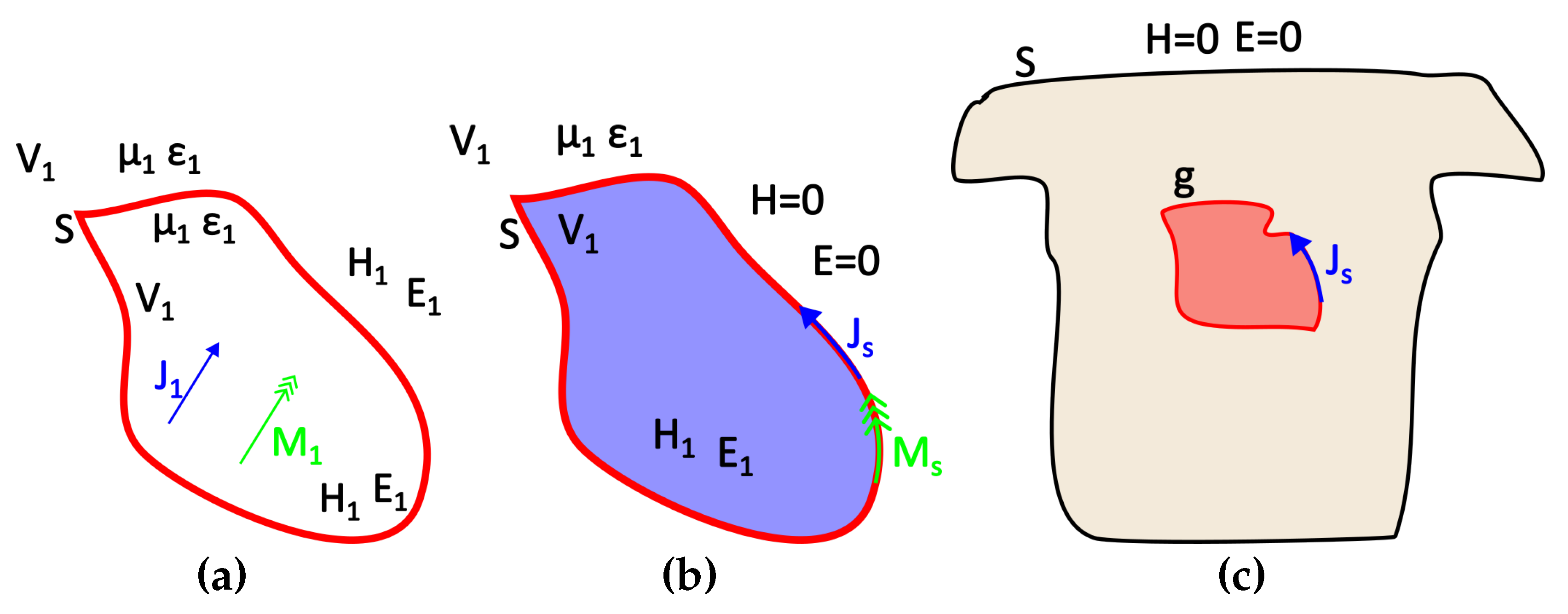
Figure 4.
The employed thorax model where (a) the different recorded sites and (b) the anticipated surface potential distribution are presented.
Figure 4.
The employed thorax model where (a) the different recorded sites and (b) the anticipated surface potential distribution are presented.
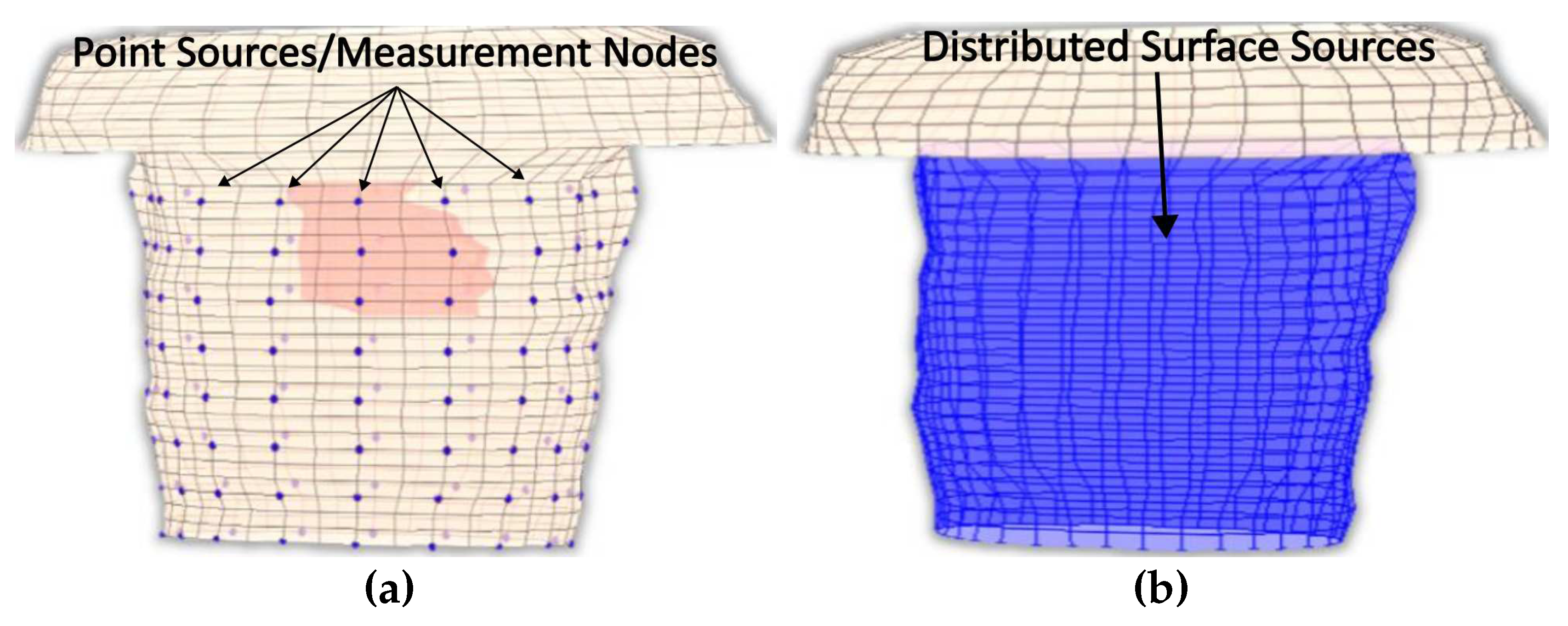
Figure 5.
The pyramidal interpolation function as denoted upon the utilized node configuration. The voltage is measured on purple nodes and is additionally sought-interpolated on black nodes.
Figure 5.
The pyramidal interpolation function as denoted upon the utilized node configuration. The voltage is measured on purple nodes and is additionally sought-interpolated on black nodes.
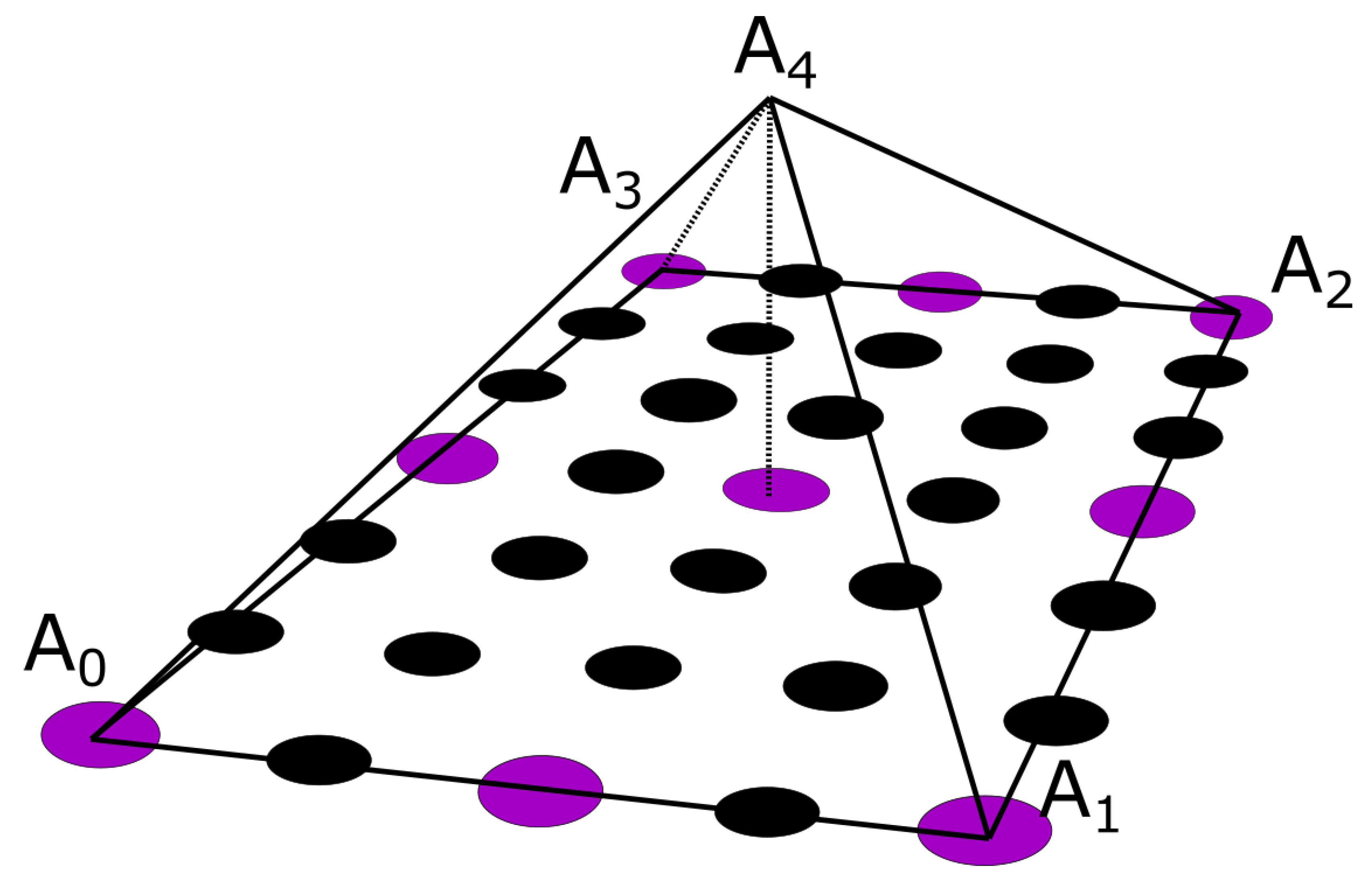
Figure 6.
(a) Eigenvalues distribution at the first 200 eigenvalues with the different energy percentage considered and (b) four indicative low order eigenvectors of thorax’s at the 20th cross-section including a slice of heart as depicted in Figure 1.
Figure 6.
(a) Eigenvalues distribution at the first 200 eigenvalues with the different energy percentage considered and (b) four indicative low order eigenvectors of thorax’s at the 20th cross-section including a slice of heart as depicted in Figure 1.
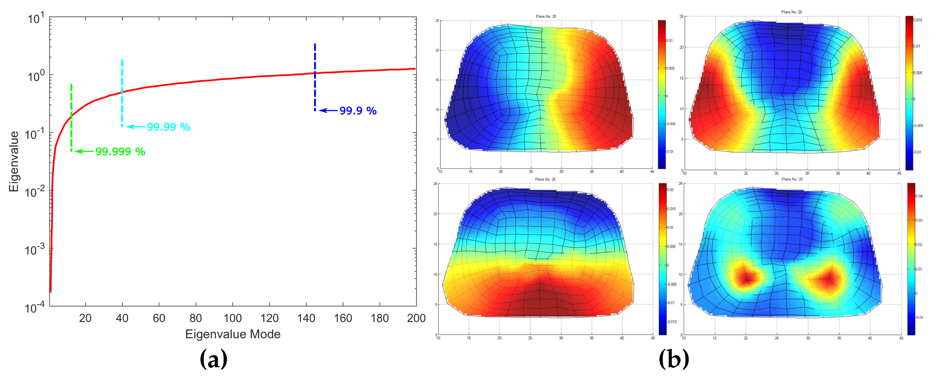
Figure 7.
The epicardium potential distribution resulted from the inverse direct method for t=8 msec, t=30 msec, t=130 msec, t=170 msec, t=200 msec, t=420 msec and t=740 msec compare to a physiological PQRST electrocardiograph.
Figure 7.
The epicardium potential distribution resulted from the inverse direct method for t=8 msec, t=30 msec, t=130 msec, t=170 msec, t=200 msec, t=420 msec and t=740 msec compare to a physiological PQRST electrocardiograph.
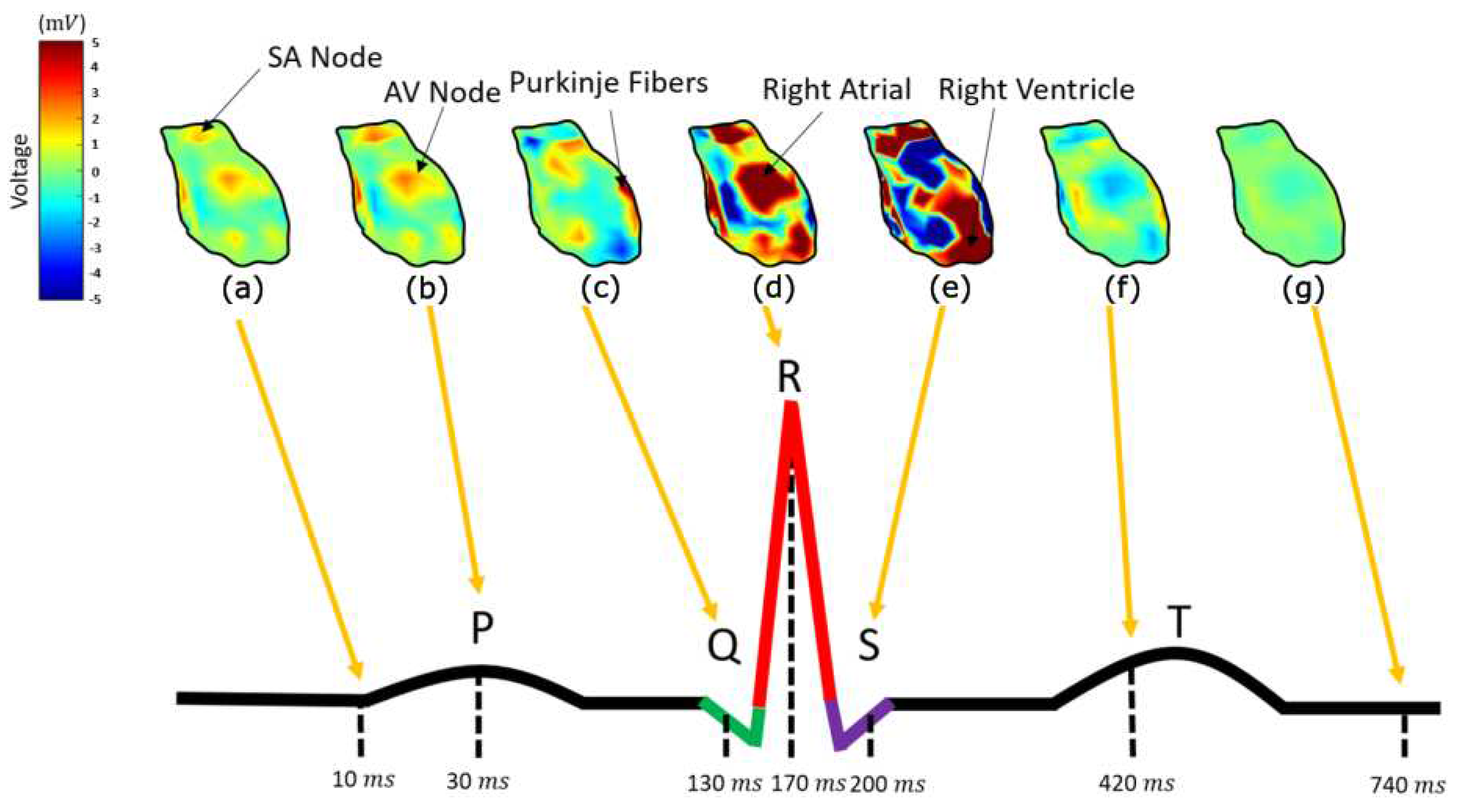
Figure 8.
Original ECG measurements versus generated potential on electrodes (a)9, (b) 78, (c) 114 and (d) 141 after the evaluation of the resulted equivalent source.
Figure 8.
Original ECG measurements versus generated potential on electrodes (a)9, (b) 78, (c) 114 and (d) 141 after the evaluation of the resulted equivalent source.
Disclaimer/Publisher’s Note: The statements, opinions and data contained in all publications are solely those of the individual author(s) and contributor(s) and not of MDPI and/or the editor(s). MDPI and/or the editor(s) disclaim responsibility for any injury to people or property resulting from any ideas, methods, instructions or products referred to in the content. |
© 2023 by the authors. Licensee MDPI, Basel, Switzerland. This article is an open access article distributed under the terms and conditions of the Creative Commons Attribution (CC BY) license (http://creativecommons.org/licenses/by/4.0/).
Copyright: This open access article is published under a Creative Commons CC BY 4.0 license, which permit the free download, distribution, and reuse, provided that the author and preprint are cited in any reuse.


