
Submitted:
25 July 2025
Posted:
28 July 2025
You are already at the latest version
Abstract
This paper presents an innovative approach to compressing and decompressing activity durations within the context of multi-project scheduling under uncertainty and resource flexibility. In dynamic project environments, fixed activity durations often restrict optimal scheduling outcomes. To address this challenge, the proposed method systematically adjusts activity durations—through compression and decompression—while maintaining resource and precedence feasibility. By integrating Critical Path Method (CPM) analysis with heuristic rules, the approach identifies candidate activities whose durations can be reduced or extended based on slack availability and resource effort profiles. The objective is to enhance scheduling flexibility, improve resource utilization, and better align project execution with organizational priorities. Validated through a case study at an automotive company in Portugal, the method demonstrates its practical effectiveness in recalibrating schedules and balancing resource loads. This contribution offers a timely and necessary innovation for companies aiming to enhance responsiveness and competitiveness in increasingly complex project landscapes. It provides an actionable framework for dynamic schedule adjustment in multi-project environments, helping companies to respond more effectively to uncertainty and resource fluctuations. Importantly, the proposed approach also supports sustainability objectives in new product development and supply chain operations. By optimizing resource usage, reducing idle time and overuse, and improving responsiveness to real-world conditions, it contributes to minimizing waste, increasing operational resilience, and aligning project execution with strategic sustainability goals.
Keywords:
Multi-project scheduling
; Activity duration adjustment
; Compression
; Decompression
; Critical Path Method (CPM)
; Resource flexibility
; Sustainability
; New product development
1. Introduction
In complex multi-project environments, effective scheduling and resource allocation under uncertainty remain critical for ensuring operational success. This study addresses these persistent challenges within the real-world context of an automotive company based in Portugal, where simultaneous industrialization projects must be managed with high precision and limited resources. The increasing complexity of automotive product development, combined with stringent delivery timelines and fluctuating demand, requires more robust and adaptive scheduling frameworks.
This work builds upon previous studies that integrated knowledge from Project Management, particularly in Project Scheduling, which aimed to determine the shortest project duration while accounting for resource capacity constraints and reducing project overruns and delays across multiple concurrent efforts (Aghileh et al., 2024; Lima et al., 2020; Pereira et al., 2018). Expanding on this foundation, the current research adopts an innovative approach that reflects recent trends in project management theory and practice. From a strategic perspective, it incorporates project activities with varying work content () to better manage uncertainty, allowing for more realistic and resilient planning.
The objective is to develop a novel approach to multi-project scheduling that blends flexibility. This is achieved by enhancing traditional scheduling techniques with dynamic resource allocation and iterative heuristics. A key contribution of this work is the application of compressing and decompressing strategies to activities with zero slack to balance the workload of project managers.
The findings of this research will offer valuable guidance for both researchers and practitioners in the field of multi-project scheduling. By synthesizing the existing body of knowledge and identifying key research gaps, the study aims to advance the development of more effective, resilient, and practical scheduling methodologies for multi-project environments.
Following the introduction in Section 1, Section 2 presents the background and literature review, with a detailed examination of resource-constrained multi-project scheduling problems (RCMPSP) and their key variants. Section 3 outlines the research methodology employed in this study. Section 4 introduces the case study, while Section 5 presents the proposed solution. Section 6 discusses the results and highlights the key findings. Finally, Section 7 concludes the study, offering insights and implications for future research and practical applications.
2. Literature Review
2.1. Project Scheduling Concepts and Models
Project scheduling is a fundamental aspect of project management, essential for organizing a set of interdependent activities under resource and time constraints. In most organizations, activities must be scheduled using a limited pool of resources, which significantly influence project costs and duration (Amirian & Sahraeian, 2017). Scheduling involves creating an optimal timeline for performing tasks or activities. It is critical across various engineering and operational fields such as job shop scheduling, system operations, and project management. A poorly designed schedule can lead to substantial economic losses, particularly in large-scale projects (Yuan et al., 2019). According to Villafáñez et al. (2019), project scheduling requires determining start and end times for all activities while accounting for precedence relations, temporal limitations, and resource constraints. The ultimate aim is to optimize project objectives—commonly minimizing duration or cost. For instance, in an aircraft development project, the scheduling objective might be to complete the project as quickly as possible (Faria et al., 2020).
The project’s constraints are critical to project scheduling and can also be closely related to the project’s scheduling objectives. They establish the conditions that must be satisfied in sequencing activities and assume two fundamental forms that can model most of existing constraints: precedence constraints and resource constraints. Precedence constraints represent the fact that some activities must precede (or succeed, which is the same if activities are inverted in the relation) some others, for whatever reason, for some amount of time. Resource constraints represent the fact that resources are finite and therefore some activities might not be executed in parallel with some others, even if they do not have any impeding precedence relation, due to the non-existence of enough available resources to execute them all (Faria et al., 2020).
Once a schedule is established—known as the baseline schedule—the project enters the execution phase. In a deterministic setting (fixed durations and resource needs), this schedule specifies when each task starts and finishes. Project managers then monitor progress and control deviations from the plan to ensure objectives are met.
Modern project scheduling methods were originated in the late 1950s with graph-based techniques such as the Critical Path Method (CPM) (Kelley Jr & Walker, 1959; Malcolm et al., 1959). These models compute project durations and activity timelines efficiently but generally assume unlimited resource availability (Villafáñez et al., 2019). To address this limitation, researchers and practitioners developed the Resource-Constrained Project Scheduling Problem (RCPSP), which integrates resource limitations into the scheduling model. The RCPSP focuses on optimizing the schedule of activities while respecting both precedence and resource constraints, typically with the goal of minimizing the project’s makespan (Hartmann & Briskorn, 2010; Sonmez & Uysal, 2015). This shift marked a significant evolution in project scheduling, making it more realistic and applicable to practical scenarios where resource availability is often a critical bottleneck.
Due to its real-world relevance and computational complexity—RCPSP is NP-hard in the strong sense (Blazewicz et al., 1983)—exact solution methods are only feasible for small-scale projects (usually fewer than 60 activities). Consequently, extensive research has focused on heuristic and metaheuristic approaches to efficiently handle larger and more complex instances (Zhang, 2012).
Building on RCPSP, the Resource-Constrained Multi-Project Scheduling Problem (RCMPSP) addresses scenarios where multiple projects must be scheduled concurrently, often competing for shared resources. First introduced by Pritsker et al. (1969), RCMPSP reflects real-world conditions where companies typically manage portfolios of projects rather than isolated ones. In addition to precedence and resource constraints, RCMPSP also incorporates project-specific release times, adding further complexity.
Like RCPSP, RCMPSP is strongly NP-hard (Marimuthu et al., 2017), and solving it for large-scale problems remains a challenge. This has spurred a growing body of research dedicated to developing advanced heuristics and metaheuristics tailored to multi-project environments (ElFiky et al., 2020; Shu et al., 2018; Yan et al., 2014).
2.2. Uncertainty
In a real environment, there is considerable uncertainty during project execution. Several factors contribute to uncertainty in multi-project scheduling. They are divided into two categories. The first kind is the uncertainty caused by the external environment, for example, adding more activities due to temporary increased orders, information uncertainty and weather conditions. The second type of uncertainty relates to production factors, known as resource uncertainty. The most common uncertainties are a temporary shortage of resources and equipment failure (Weixin et al., 2019).
During the project execution, uncertainty is the main factor that frequently affects the baseline scheduling plan, resulting in delayed start times and interruptions to resource supply. As an example, project duration may change due to a temporary change in activity duration, a new activity introduced during project execution and the cancellation of the original activity. Consequently, the entire project scheduling process becomes difficult to control (Weixin et al., 2019). Approximately 5% of scheduling time is spent developing new schedules, while 95% is spent revising and maintaining schedules as daily progress and assumptions change, according to Fox and Ringer’s survey (Zheng et al., 2013).
Uncertainty factors may affect a multi-project scheduling scheme in more complex ways, and at any point during project execution. A multi-project scheduling plan cannot accurately predict the completion times of each activity, thereby weakening its performance. Uncertain factors have been shown to have a significant impact in how robust scheduling is and greatly increases the risk of delays (Weixin et al., 2019).
Due to resource constraints, when two or more dynamic factors, such as stochastic duration and new project arrivals occur simultaneously, they significantly impact baseline scheduling. Addressing this type of dynamic RCMPSP, Chen et al. (2019) indicate that a stochastic environment is more realistic, as it better represents real-world conditions (ElFiky et al., 2020). Therefore, stochastic scheduling has received widespread attention in RCPSP to deal with uncertain activity durations, but there is a lack of literature about RCMPSP with stochastic activity durations. In general, RCMPSP in stochastic environment is far more complex than in a deterministic one.
A number of surveys examined the fundamental models and approaches to scheduling projects under uncertainty and provided insights into potential research areas (Wang et al., 2015).
2.3. Resource Flexibility
By allowing flexibility resource allocation, the new problem becomes a generalization of the RCPSP. Hence, its optimal makespan is at least as good as the makespan of RCPSP. Under these new circumstances, the resource usage at any time and the duration of each activity are unknown a priori and, thus, they need to be simultaneously determined while scheduling activities by their starting times. This problem is termed here as the RCPSP with Flexible resource profiles (FRCPSP) (Naber & Kolisch, 2014).
This problem is firstly introduced by Kolisch et al. (2003) for an application in pharmaceutical research. Despite its tremendous potential, the problem has not yet been well-studied, as compared to the RCPSP. Recently though, the FRCPSP has attracted wider attention from researchers, who subsequently proposed different model formulations and heuristic methods.
While in the RCPSP the resources are allocated in constant amounts over the entire duration of each activity, Kolisch et al. (2003) proposed a model in which resource allocation must be determined. In Ranjbar and Kianfar (2010) proposal, RCPSP-FWP (RCPSP with Flexible Work Profiles) is used in the same meaning as FRCPSP. The RCPSP-FWP is a different version of the well-known RCPSP, which consists of interrelated activities with a zero-time lag that are interconnected via finish-start type precedence relations. In this case, a single renewable resource is available and activity duration and resource usage to a single renewable resource are known constants.
As a result, relative to the work profile, the ‘‘work content’’ (Fündeling & Trautmann, 2010; Tereso et al., 2004) is defined as the total amount of work required to complete an activity. The total work content of each activity is given, instead of the duration and resources required for each activity, which essentially indicates how much work needs to be done. In other words, activities’ durations and resource usages at any time are unknown. FRCPSP assumes that activity duration is not set, being part of the problem to be solved (Ranjbar & Kianfar, 2010).
To proceed, the concept of work content () is given by expression (1), where is the duration of activity and is the amount of effort (Tereso et al., 2004).
As an example, a work content of 10 man-days for an activity may be allocated into a constant profile of 2 men for 5 days, as per an RCPSP approach, or into a flexible profile of 5 men for 2 days and 1 men for 20 days.
Fündeling and Trautmann (2010) and Baumann et al. (2015) considered flexible resource profiles as well. In their approach, a single work content resource is given for the project.
The RCPSP-FRM approach proposed allows a critical activity, with no slack, to be reduced in duration by using a strategy to decelerate non-critical activities, with slack, placing them in a slower work mode, so critical activities, which may increase in duration, may still run simultaneously, using their resources at a faster pace. Due to the evolution of the methods used to solve this issue, many more studies are still required to enhance the efficiency and effectiveness of projects (Faria et al., 2020).
2.4. Sustainability
Sustainability has garnered significant attention within academic research, attracting a substantial and growing body of literature (Caniato et al., 2012; Lee & Farzipoor Saen, 2012). Central to this discourse is the “profitability triangle”, a conceptual framework predominantly applied to corporate contexts (Gmelin & Seuring, 2014). This framework encompasses three interrelated dimensions: economic profitability, environmental protection, and social responsibility.
The profitability triangle has been regarded as a practical tool for organizations seeking to operationalize the Brundtland Commission’s definition of sustainable development, which describes it as “development that meets the needs of the present without compromising the ability of future generations to meet their own needs”. This triple bottom line approach is particularly relevant in the context of supply chain management, where sustainability efforts must address economic, environmental, and social impacts across the product life cycle (Gmelin & Seuring, 2014).
Sustainable product development aims to fulfill user needs while minimizing negative environmental and social externalities and simultaneously delivering economic value to the company (Hsueh, 2011). As such, sustainability has been identified as a potential source of competitive advantage, influencing not only individual companies but also the broader supply chain (Caniato et al., 2012). Shrivastava (1995) offers a more environmentally focused interpretation of sustainability, emphasizing the mitigation of long-term risks linked to resource depletion, energy price volatility, pollution liabilities, and waste management. However, this perspective is often critiqued for overlooking social performance aspects—a limitation repeatedly highlighted in the literature (Mu et al., 2011).
2.5. New Product Development (NPD)
Research in New Product Development (NPD) has been of interest for several decades (Wind & Mahajan, 1988). NPD attracts researchers being interested in engineering (Perrone et al., 2010), collaboration aspects (Emden et al., 2006), with regard to globalization efforts (Townsend et al., 2010).
New product development indicates a transformation of a market opportunity and a set of assumptions about a product technology into a product available for sale with cross-functional integration and quick development cycles (Brown & Eisenhardt, 1995; Krishnan & Ulrich, 2001; Marion et al., 2012). Following a market opportunity is essential, which nowadays is asking for products with sustainable characteristics.
Sustainable products, however, require internal and external interaction and collaboration in new product development (Tan & Tracey, 2007). Consequently, collaboration in NPD processes across companies may provide long-term advantages for a new product development (Gmelin & Seuring, 2014).
NPD is the process of bringing a new product or process to the marketplace. All the activities related to development of the new product including idea generation, screening, testing and getting customer approval happen in NPD life cycle. In every industry, NPD process has significant value because it greatly influences the whole value chain and decisions on fundamental aspects such as quality, cost and time. Companies can achieve competitive advantage by differentiating their final output through product and process innovation (Gmelin & Seuring, 2014).
Organizations struggling with NPD challenges—such as prolonged project timelines, underperforming product launches, or an overburdened development pipeline—should consider transitioning to a fifth-generation Stage-Gate system. Over the past four decades since its inception, the Stage-Gate model has undergone significant advancements, with leading companies continuously refining their gating processes to enhance efficiency, responsiveness, and innovation outcomes.
The Stage-Gate process is a widely recognized framework used by organizations to manage NPD projects in a structured, disciplined, and transparent manner. First introduced by Cooper in the early 1980s, the model breaks down the innovation process into a series of well-defined stages—each representing a set of activities—separated by decision points known as “gates” (Cooper, 2022). At each gate, a cross-functional management team assesses the project based on predefined criteria and decides whether to proceed, revise, delay, or terminate it.
As innovation challenges have evolved, so has the Stage-Gate process. The 5th Generation Stage-Gate model addresses key issues facing companies today, namely, increasingly compressed timelines, higher product complexity, the need for sustainability, and dynamic market conditions. This new generation of the Stage-Gate system integrates lean principles, parallel processing, iterative development, and Agile methodologies to enhance both speed and effectiveness in NPD (Cooper, 2022).
2.6. Integration of Sustainability in NPD Scheduling
In today’s competitive and environmentally conscious industrial landscape, sustainable product development is no longer limited to the characteristics of the final product—it extends to the efficiency and responsibility with which projects are executed.
The NPD process traditionally involves collaboration across multiple internal functional areas, including Research and Development (R&D), marketing, finance, supply chain, and manufacturing. In today’s competitive and increasingly sustainability-conscious global market, companies are encouraged not only be innovative but to do so in a manner that creates new customer value while ensuring environmental and social sustainability (Bevilacqua et al., 2007).
Customer expectations for sustainable products are on the rise, alongside increasing governmental regulations aimed at promoting products with sustainable attributes. Products characterized by sustainable features can offer a significant competitive advantage. While many companies claim to offer sustainable products, from an academic standpoint, such products are often still seen as lacking in efficiency with respect to sustainability criteria (Kleindorfer et al., 2005). The integration of sustainability into NPD remains a complex challenge, especially when balancing corporate sustainability objectives with often divergent customer demands and preferences (Keskin et al., 2013). Therefore, it is imperative to identify and implement strategies that effectively support sustainable NPD.
Product development is often considered the “nexus of competition”, as it shapes the product’s performance throughout its lifecycle and underpins a company’s long-term success. In light of this, developers are increasingly called upon to integrate sustainability into the early phases of NPD (Gmelin & Seuring, 2014).
The principal challenge for sustainable NPD is to enhance product sustainability without incurring additional costs or complicating production processes. Sustainable product development, therefore, refers to the process of creating products or services that are improved in terms of sustainability for market deployment (Bhuiyan & Thomson, 2010).
3. Research Methodology
This study adopts a Design Science Research (DSR) methodology to develop, implement, and evaluate a heuristic-based scheduling tool aimed at compressing and decompressing activity durations in multi-project environments under uncertainty and resource flexibility. DSR is especially suited for addressing practical problems through the creation of innovative artifacts that provide solutions grounded in theoretical foundations (Hevner et al., 2004). In this research, the developed artifact is a decision-support tool that aligns with the dual objectives of operational efficiency and sustainability in project management.
Following the DSR paradigm, the research process is structured into three interdependent cycles: the relevance cycle; the design cycle; and the rigor cycle. The relevance cycle connects the research to the real-world environment through an applied case study in a Portuguese automotive company. This organization provided the empirical context and constraints—including activity networks, project categories, resource data, and Quality Gate Checkpoints (QGCs)—necessary to inform problem definition and tool requirements. The design cycle was dedicated to the iterative development of the heuristic algorithm and the supporting Python-based software. The rigor cycle ensures scientific grounding, drawing from prior literature in RCMPSP, CPM, and flexible resource allocation models such as FRCPSP and RCPSP-FRM.
To ensure methodological clarity, the research design also integrates the “Research Onion” model by Saunders et al. (2019), which guides the philosophical and strategic choices behind the study. At the philosophical level, the research adopts a pragmatic stance, valuing both objective efficiency and contextual relevance. At the approach level, it follows an abductive logic, iterating between empirical observations and theoretical frameworks to develop a robust solution. The methodological choice is mixed-methods, combining computational modeling and qualitative validation via focus groups. The research strategy involves an embedded single-case study design, grounded in the operational processes of a real organization. Finally, data collection was conducted through company documentation, expert interviews, and operational system outputs, and supported by algorithmic simulation and analysis.
The artifact was implemented as a scheduling tool designed to dynamically adjust activity durations via compression and decompression logic. Compression was applied to critical path activities when the latest finish exceeded QGC deadlines, while decompression was introduced either for non-critical path activities to balance workload or to extend durations where slack was available. This approach ensures adherence to target deadlines without overburdening resources. The tool calculates key parameters such as ES, EF, LS, and LF using CPM principles. It then applies a priority-based heuristic to determine which activities to adjust based on resource profiles, slack, and sustainability constraints.
The tool was evaluated using real project data from three concurrent industrialization projects. Metrics such as schedule adherence, resource utilization, and effort distribution were tracked to assess performance. To validate the tool’s practical relevance, a focus group was conducted with key stakeholders, including project managers and planning engineers. Participants provided feedback on usability, visual dashboards, and decision-making support, which led to refinements in the final version of the tool. This participatory approach ensured alignment with organizational needs and enhanced the artifact’s applicability in dynamic, sustainability-driven project settings.
Overall, the research methodology integrates theoretical depth with practical applicability, ensuring that the developed scheduling tool not only addresses academic gaps in RCMPSP under uncertainty but also delivers actionable insights for industrial practice.
4. Case Study
The company where this study was done is one of the most recognized companies in Portugal, dedicating itself to the development and production of infotainment systems, instrumentation and safety sensors for the automotive industry, as well as developing solutions for connected and autonomous mobility.
The study was developed in the Manufacturing Engineering (MFE) department, which integrates several sectors, for example, project management, sample development, assembly, testing and maintenance (Pereira, 2018), aiming to support the management of industrialization projects. An industrialization project is related to the design of the manufacturing line to produce a certain product, aiming to reduce costs and increase the production capacity of the manufacturing line (Aghileh et al., 2022; Perrotta et al., 2017). In the case study, an industrialization project manager (iPM) can manage more than one project simultaneously, depending on their complexity. The resources that are the focus of attention during this study are precisely the iPMs.
Projects in this context have a “Category”, depending on the complexity of the project, and during the industrialization project, several “Samples” can be made, to be sent to the costumer. Project categorization is according to their impact on the operating unit and can be classified as: A, B, C and D, with the most complex being A and the least complex being D. Each classification, in turn, has its respective level of complexity, with the most complex being A and the least complex being D.
There are also five types of sample phases that can be grouped as (A, B, C, D), (A, C, D), (B, C, D), (C, D) or (D). In different choices, different prototypes are constructed and introduced.
In a different dimension, there are the dates of the project’s deliverables, that is, the records relating to the dates of the QGCs (QGC is conducted at predefined points in a project’s lifecycle to ensure that all project management requirements are fulfilled before proceeding to the next phase), the beginning and end of the project.
The QGCs are named such that the first is referred to as KOD (Kick-Off Design), the second as KOP (Kick-Off Plant), and from the third onward, they are labeled as QGC followed by a sequential number starting from zero. Therefore, the activities in phase 0 are located between KOD and KOP.
A description of the activity networks of category A will be made, since this category is the most complete one, and others have the same structure, but some activities are not done (duration 0).
Category A is made up of 147 activities and seven project phases (Figure 1). This structure is also applied in a similar way in categories B, C and D, with different samples, that is, with different activities, according to the complexity of the project.
It is important to highlight that, even if a project is unique, for simplification reasons, although the activities are similar, there is a variation in terms of duration and effort applied to carry out the activities. It is also important to mention the direct relationship that exists between the duration and effort (amount of resources allocated) to carry out an activity, which was discussed in Section 2.3.
To clarify more, first of all, the Program Manager (PgM) can choose the categories A, B, C, or D. After selecting a specific category, one type of sample is chosen from the options (ABCD, ABC, ACD, CD or D). Then, any activities that are not part of that sample are excluded. The duration of these excluded activities is considered zero in the calculation. By determining the duration and efforts, the Work Content (WC) for each activity was calculated.
5. Solution Proposal
Building on Aghileh et al. (2024) systematic literature review and Aghileh et al. (Aghileh et al., 2025), this study introduces a heuristic-based approach to address compression and decompression strategies within the RCMPSP. The methodology is applied to real-world project scheduling data provided by a major automotive company, encompassing multiple interrelated projects with shared resource constraints. The primary objective is to optimize project schedules by distributing the resources equitably to meet stage gate deadlines, achieved through a strategic combination of activity compression and decompression.
The approach focuses on the critical path. Compression is applied to activities on the critical path to shorten project duration directly, while decompression is used on non-critical activities to introduce flexibility without affecting the makespan. Alternatively, if decompression is necessary on critical path activities—such as for robustness—compression is not applied to non-critical activities to preserve the overall schedule length. This balance ensures that any schedule relaxation does not compromise the global optimization goal.
The approach was implemented in a Python-based framework.
Key performance indicators, such as total project duration and resource utilization, are tracked and analyzed across multiple iterations. The proposed method is evaluated from the automotive dataset, enabling validation in a realistic industrial setting. The results aim to provide practical insights into how heuristic scheduling can enhance operational flexibility and efficiency in complex, resource-constrained environments.
5.1. Construction of Schedules in the Developed Tool
The general structure of the proposed heuristic is depicted in Figure 2, and the details of the developed algorithm are then detailed.
At the beginning, the heuristic begins with the definition of the parameters of the model which consists of attributing the properties of project activities from different categories, namely, the duration of each activity, the amount of resource that each activity requires throughout the period of its execution and the precedence relationships that characterize the generic activity network.
Additionally, there is another type of parameters necessary for the algorithm, the input parameters. The first input parameter to be mentioned is the “current date”, that is, the date on which the business plan in question occurs and from which all planning is done.
It is still necessary to enter input parameters relating to the most specific information for each project. This information comes from documentation relating to the project portfolio under analysis in the ongoing business plan, and is detailed in Table 1.
The ID and name of the project are merely important for identification reasons. The type of project excludes from consideration all projects that do not belong to the group of industrialization projects, since the heuristic presented applies exclusively to this type of projects. Table 2 illustrates an example of the input parameters.
5.2. CPM
Through the CPM, the tool can calculate the Earliest Start (), Earliest Finish (), Latest Start (), Latest Finish (), and slack time with the consideration of the predecessors.
To calculate the CPM, the process begins by defining all the activities necessary to complete the project, along with their durations. Each activity is then examined to determine its predecessors —that is, which activities must be completed before it can begin. Once the predecessors are established, a project network is constructed. With the network in place, the next step is to perform a forward pass through the network to calculate the and times for each activity.
It was proposed that scheduling be done so that all activities begin at their earliest start time, that is, at their (assigning the of initial activities equal to zero).
Firstly, the of the activity in phase 0 in the project is determined through calculation (equation 2), following what is typically called forward-pass and where is the duration of activity in project .
For subsequent activities, the is determined by the maximum of all its immediate predecessor activities, where . represents the set of activities that come before any activity .
When the EF of the last activities of a phase are evaluated, the ES of the first activities in the next phase are equal to the maximum EF of the last activities of the previous phase and this process will be repeated for all phases of the project.
The tool records the start and end information of each phase, because the end time of will be the start time of . For example, if activity 7 that belongs to phase 0 is completed at time 10, activity 8 will also start at time 10. Each phase is understood as a phase that needs to respect the established due dates, and its end date will be considered as the start date of the next phase.
Using the reverse path, called backward-pass, for activity in project the calculation of and begins using the formula presented in equation 3:
where , for the last activity. Equality defines that the of the last activity corresponds to its .
where . represents the set of activities that follow any activity .
The four variables explored so far are useful for calculating the slack of each activity of a project , given by equation 4:
This value allows understanding which activities belong to the critical path (activities with 0 slack), that is, the activities whose change in duration (adjusting to the problematic context under study) causes changes in the project completion date. All paths in the scenario under analysis must be worked on. Expression 4 calls up the and of an activity to calculate its float. However, the same slack value would be obtained if the latest start and earliest start values were used. What defines whether the activity belongs to the path is, therefore, is the value of its slack (equation 5):
where is the set of activities that belong to the critical path in project . From equation 5, it can be seen that the slack only takes a null or positive value.
Applying the process described above, a baseline schedule was created. It was the first process to create a project schedule for the solution, using the developed heuristic approach.
5.3. Compress and Decompress for Activities with Slack=0
Networks are guided by the dates on which quality-gates are validated. These dates are imposed by customers and compliance with them will be the fundamental constraint of the model. Referring to the fundamental restriction of the model -respecting the QGC dates- it is important to understand the reason why compliance may not be possible. The answer lies in the duration of the activities. In fact, the longer the activity durations, the later a project will be completed. It is easily understood that the way to get around the issue of dates imposed for validating the QGCs is to manipulate the duration of the activities. However, from expression 1, it can also be seen that a change in the duration of an activity has an impact on the amount of resources required for its execution. It is precisely the proportionality between these two factors that will determine the number of resources needed to execute a project within the deadlines established by quality-gates.
In this new instance, the tool checks whether it is necessary to compress or decompress the initial solution for project activities durations. The difference (in days) between the date of each QGC and the respective is calculated, assuming that in the initial baseline all activities are scheduled to begin at their earliest start, that is, without delays. This value is stored in two integer variables called compress and decompress and defined by (equations 6 and 7) which means that in project , compressing/decompressing is the difference of of the last activity in a phase and the respective :
If the maximum of the activities in a phase exceeds the respective quality-gate date, the compress variable takes on a positive value and the durations of certain activities must be compressed (the critical path activities). Conversely, if there is a gap between the maximum and the due date, the compression variable takes on a negative value. Consequently, the decompress variable takes on a positive value and the durations of certain activities will be extended. In both scenarios, the duration of each activity, as an input parameter, will be changed, which will require an adjustment in the effort required for their performance. From equation 1, it is clear that the effort will increase if it is necessary to compress activities and will decrease otherwise.
It is now important to find out how durations are increased/decreased, as well as the priority rule associated with the selection of activities subject to change. Since the performance of activities is assumed on a daily temporal basis, it was defined that it would be removed/added day by day to its durations. Although it was mentioned previously that the activities on the critical path would be the activities to be considered, it is necessary to bear in mind that the amount of time to “compress/decompress” may not be considerable. This implies that only some of the activities on the critical path undergo changes.
Even in the scenario where it is necessary to comply with the base schedule, if it is necessary to compress more than one day, more activities are considered to reduce the respective duration. Thus, all activities on the critical path are listed in ascending order according to the logic explained previously. From that point on, the list is scrolled, removing 1 day of duration from each activity, one by one, until the compress variable equals the value 0.
The reverse logic applies if it is necessary to decompress the baseline schedule, since there is a gap between the maximum earliest finish of the activities in a phase and the respective quality-gate.
If the number of days that needs to be reduced is less than the number of activities that belong to the critical path, when the number of days that needs to be reduced is reached, the tool stops removing days from activities. If the number of days that needs to be reduced is greater than the number of activities that belong to the critical path, one day is first subtracted from each activity. After this adjustment the critical path is recalculated. If further reduction is still needed, the process continues—removing one day at a time from the updated set of critical activities—until the project’s end date aligns with the target date. It is important to mention that as activities are compressed, the work content of each activity is maintained, that is, to reduce the duration of activities, a greater effort needs to be carried out. It is also important to mention that the rule was used that no activity should exceed the value of 1.2 (120%) of daily effort (20% more than usual is acceptable) or less than 0.05, to accommodate a potential risk of creating an unenforceable schedule.
It is important to know for instance, if the target completion date for Phase 0 ends on KOP is 2025/08/10, this phase should be completed by the end of the day on 2025/08/09. If 2025/08/09 falls on a holiday or weekend, however, the phase completion should be adjusted to the last working day prior to that date.
In “decompression” overview, activities are listed in descending order of resource usage, when they are scheduled. The first activities on the list will be prioritized to increase duration and, consequently, decrease in terms of resource usage.
After making the necessary changes to the duration of the activities so that the quality-gates are respected, the activities will be scheduled again between their earliest start and their earliest finish, according to the new duration values. Likewise, the resource profile is updated according to the new effort values.
The last iteration of the heuristic, also called the model stopping criterion, checks whether the due date is respected after the changes and, if so, the algorithm ends. Otherwise, the process repeats.
5.4. Compress and Decompress for Activities with Slack≠0
In the previous section, the focus was on activities with slack equal to zero along the critical path, aiming to align the project with the date suggested at the beginning of the process. In this section, to offset some or all the adjustments made earlier, it was conducted compression and decompression operations on activities with non-zero slack.
The method is as follows: if compression was applied to zero-slack activities, decompression must now be applied to non-zero slack activities. During compression, the duration of zero-slack activities was reduced, which, given the fixed work content, necessitates an increase in effort. Therefore, the prioritization of activities is performed in descending order based on the maximum recorded resource usage. Subsequently, one day is added to the duration of each selected activity in sequence, and after each adjustment, all related dates, slack values, and efforts are recalculated.
To keep balance, the total effort added in the prior section was calculated and the process continues until the added effort is minimized through decompression of non-zero slack activities accordingly.
Conversely, if decompression was applied to zero-slack activities previously, now the process is complete and the due date was reached and there is no longer a need to apply compression to non-zero slack activities.
For further clarification, a practical example of this concept is provided in the following section. This example will help illustrate the application of compression and decompression adjustments on activities with varying levels of slack, demonstrating how these operations affect the overall project timeline and resource allocation.
6. Results and Discussion
6.1. Results
In this section, an example of a simple scenario will be introduced to clarify how the heuristic was implemented and how the algorithm works.
The scenario was designed, in the simplest way possible, in order to explain the concepts of heuristics and their application in a variety of concrete situations. In this sense, what follows is an example that focuses on pertinent details of the heuristic, combined with its general functioning.
Since a multi-project environment is being examined, three projects, each consisting of 147 activities, were investigated, and to simplify the analysis, one small section from one of the projects (a phase) (between KOD and KOP) has been selected to allow the details of the algorithm to be explained.
The example was explored according to a description that accompanies the heuristics presented in the previous section, step by step. Simultaneously, brief references are made to the code that supports its implementation at the computational level. This was developed in Python programming language.
The first two parameters (ID and name) are only useful for reference and project identification purposes. As several types of projects can be analyzed in a business plan, it is necessary to rectify whether the project in question is part of the group of industrialization projects, since the present research/heuristic is intended exclusively for this type of project.
As mentioned previously, it is assumed that all projects call for the same activities and that, in all of them, these have the same interdependencies. The QGC dates work as a starting point for the next iterations of the heuristic, as can be confirmed below.
According to Table 3, the earliest start date of the first activity in phase 0 corresponds to the validation date of quality-gate.
6.1.1. CPM
Knowing the duration of each activity and following the CPM, it was possible to complete the filling of the network regarding the forward-pass. It is important to reinforce the idea that, according to the CPM method, the value of an activity is equal to the value of the respective precedence. In situations where the activity has more than one precedence, its equals the maximum value of the respective precedences.
The maximum of the activities in each phase, defines the QGC completion date. It was assumed that this is the date that must comply with the QGC, which could also be a limitation of the process, since it assumes an optimistic profile that disregards possible delays in the execution of activities. In this sense, calculating the and for each activity is only useful for later calculating float/slack.
Focusing now on the backward-pass, which corresponds to the calculation of the and , it is important to note that it uses as its initialization value the value of the last activity of each network (as is traditionally done using the CPM method). Even though it was expected to use the date of the QGCs as a reference value for calculating slack, if this same date did not coincide with the date of the last activity, all activities would have slack. Given the algorithm designed, what defines whether an activity belongs to the critical path is whether its float value is equal to zero. How this point was circumvented will be explained in the next iteration of the heuristic. To conclude this iteration, it remains to demonstrate how the , and slack values are calculated.
Therefore, using the CPM, it was established that the of the last activity coincides with its . From the value, it is possible to calculate the value of the activity by subtracting its duration. This reasoning applies to all activities, and for all activities except the last one, the equals the of its successor activity. If there are activities with more than one successor activity, the activity in question takes as its value the minimum value of the respective successor activities.
There are the slack values for each activity that result from the difference between the and the of the respective activity.
Please note that in this calculation, national holidays and weekends are not included and only working days are considered.
Following the CPM, the critical path of each of the networks was defined, represented in Table 4.
6.1.2. Compress and Decompress for Activities with Slack=0
The “decompress” variable consists of the difference between the QGC and the maximum EF of the activities in that phase. On the other hand, the “compress” variable consists of the difference between the maximum and the quality-gate date after the last network activity. Both variables indicate the slack (positive or negative) that each phase has, indicating whether it is necessary to compress or decompress the baseline. In the specific case of the example presented, according to the expression (6) and expression (7), the values of “compress” and “decompress”, for KOP, are obtained by the following expressions (8, 9):
The calculations presented previously only apply with the days of each date. After its determination and depending on the values that the variables contribute, the heuristic proceeds along two different paths. It is at this moment that the algorithm holds the first logic gate, where it is tested whether the “compress” variable is positive. If so, you need to compact the baseline, and the entire procedure is explained below.
- Sort activities by descending order of resource usage
Before explaining the iteration, it is worth noting that it was initially stipulated that the activities subject to change would only be activities on the critical path. Based on theory, these are the only ones that affect the QGC completion date.
From what can be seen in Table 4, the critical path is made up of activities 1, 2, 4 and 5. These are the only activities subject to duration changes when compressing or decompressing the schedule. Since, in this scenario, it is necessary to compress the baseline, the activities in question will experience a reduction in their durations which, consequently, will increase the need for resources that each one requires. In this sense, and with the aim of balancing the use of resources, it is important to prioritize activities that require less use of resources.
In this way, the activities are ordered as follows: using the allocation matrix, for each of the activities, the lowest resource usage value is recorded among the different values at each instant , comprised between the earliest start and earliest finish of the respective activity (if the amount of resource usage of two/multiple activities is the same, priority is given to the activity with a smaller number). Based on this value, available in Table 5, the activities are ordered in ascending order, prioritizing the activity with the lowest recorded usage value.
For the example presented regarding phase 0, Table 6 is used to clarify what was previously explained.
To conclude the explanation of this iteration, it should be mentioned that the logic associated with phase 0, phase 1, etc. is the same. However, since the objective is to decompress the baseline, that is, extending the duration of activities and, consequently, reducing resource utilization rates, prioritization is done in ascending order according to the maximum recorded value of use throughout its execution period.
- Reduction in the duration of activities and determination of new resource usage values
This phase follows a process itself composed of a set of iterations, characterized by a sequence of subtractions from the duration of the activities. Since the time base associated with the duration of activities is daily, it was assumed that, in each iteration, one day should be subtracted, so that durations that were completely out of phase with the collected values were not obtained.
An important note is the fact that there is a requirement imposed by the organization that dictates that an activity must not reduce its duration to less than one day. This aspect can be verified for activity 1, 2 and 4 in Table 7, which maintains its constant and unitary duration from the first iteration onwards. In this context, there is no longer any condition created, which could effectively be another limitation of the model. In fact, the mismatch between the completion date and the quality-gate can be such that it results in decrements that lead to unreasonable durations.
After the new durations were determined, the new resource use values were calculated, using equation 11, knowing that the work content of each activity () was maintained. As an example, equation 11 shows the calculation of this new value for activity 5 ().
The new resource usage values for other activities are visible in Table 8. Observing the values in Table 8, it is clear that the compression of the baseline causes an increase in resource usage during the execution period of all activities, as expected.
Given these changes, the Allocation Matrix no longer makes sense as it is. Thus, it was necessary to go through the activities of the project in question and, for each one, between its earliest start and earliest finish, subtract the previous resource usage value. Therefore, it was necessary to update the matrix with the new allocation values and it is in this sense that the following iteration of the heuristic arises.
- Calculation of new values for earliest start, earliest finish, latest start and latest finish
This iteration marks the heuristic because it is crucial in updating the Allocation Matrix after schedule adjustments. The way to obtain values follows the principles presented previously. Thus, in Table 9, the network for phase 0 is presented, with the updated earliest finish, latest finish and float values.
The conclusion that stands out is the fact that a comparison between Table 4 and Table 9 reveals that in Table 4, the project finishes by the August 12th, whereas in Table 9, it is scheduled to be completed by the August 11th. This indicates that the project currently exceeds the desired completion date by one day. Therefore, a one-day compression is required to meet the target deadline. Considering that in Table 4, the 12th corresponds to day 6 (maximum EF of the QGC0), the 11th can therefore be considered as corresponding to day 5.
6.1.3. Compress and Decompress for Activities with Slack≠0
Another relevant aspect is inherent to activities that do not belong to the critical path. When comparing the networks in Table 4 and Table 9, it is clear that the effort of the activities that were on the critical path has increased by 0.065 (from 0.570 to 0.635). So now it can be subtracted up to 0.065 from the effort of activities that are not on the critical path (from 0.608 to a maximum of 0.543). Of course, it should be noted that the slack of the activities is not negative and that we do not exceed the suggested date. For this purpose, the same principles related to decompression should carried out. However, as the effort cannot be reduced below a minimum threshold of 0.050, the duration of any activity cannot be increased. However, if one more unit was increased, it would exceed the proposed date. The results are presented in the following table.

Table 10.
Effort of activities in critical path before and after compressing.
| Activity number | Effort_before | Effort_after |
| 1 | 0.060 | 0.060 |
| 2 | 0.250 | 0.250 |
| 4 | 0.130 | 0.130 |
| 5 | 0.130 | 0.195 |
| Total effort | 0.570 | 0.635 |
| Difference | 0.065 | |
6.1.4. Tool Overview
Basic information for each project is stored in a file named “BaseInfo”. This file contains “QGC name”, “activities name”, “precedencies”, “duration needed in each category and sample” and “effort” of each activity.
When Python is run, the project information such as the project name, project type, category, sample, start date and the start dates of each phase must be filled.
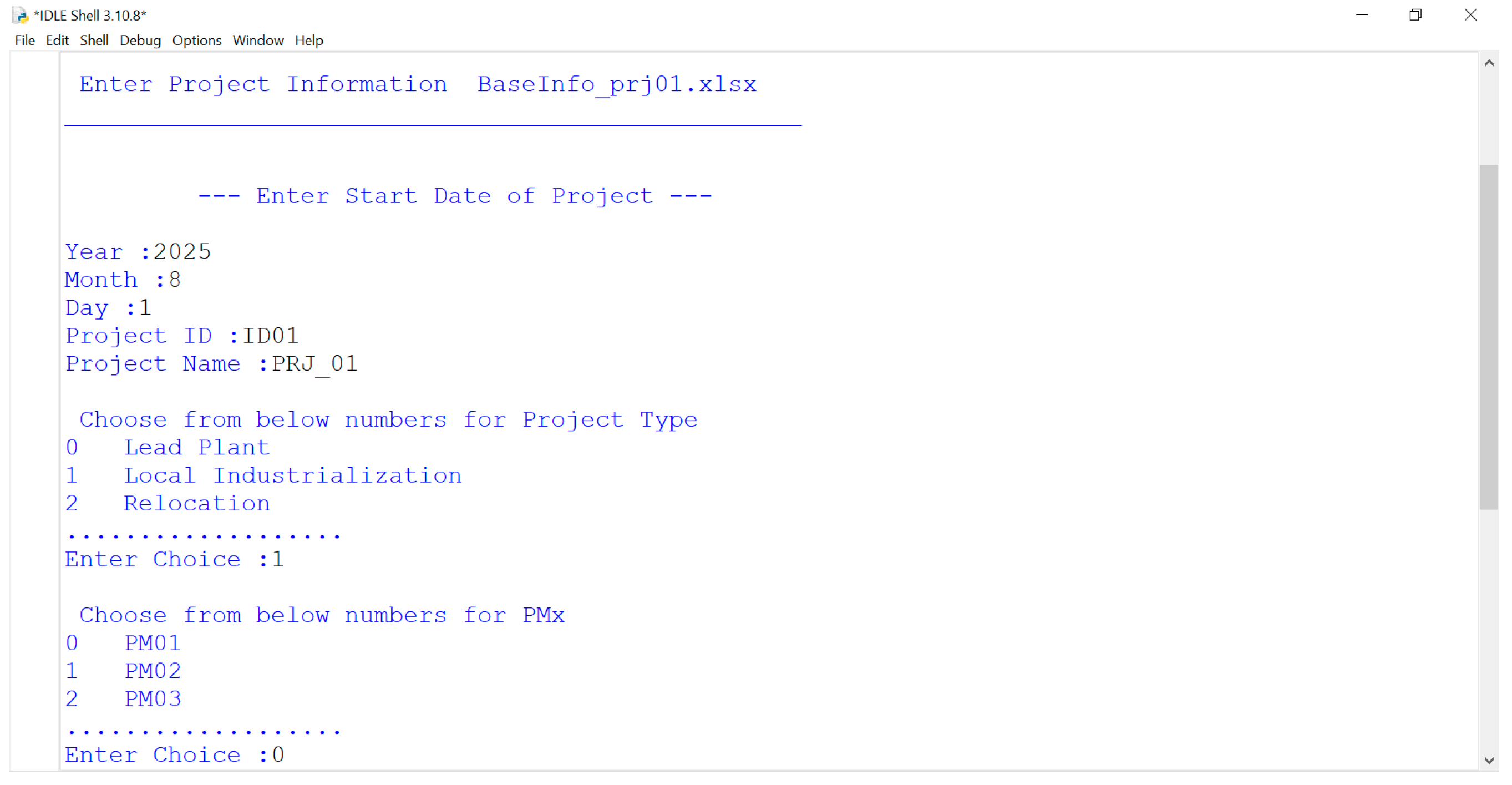
Figure 3.
Overview worksheet.
After that, the file “output_prjXX” is created, and “XX” is the number of the project that the user has inserted at the beginning. This file includes the forward path, backward path, slack values, WC and other data points that have been updated accordingly.
The entire process was conducted for each of the three projects, and the resulting data is provided below for visualization purposes. To create the graphs, several columns needed to be compiled in an Excel file named “Project_Pool” (Table 11). This worksheet contains comprehensive information regarding the effort allocated to each project, organized by month and year. This structure allows for a clear overview of effort distribution over time, facilitating project tracking and resource management.
In the worksheet named “Manager_Pool” it will be found all the information about the manager’s name and how busy the manager is each month for the projects he has to manage. According to Table 12, since iPM02 has two projects, the efforts for these were combined into a single column, resulting in a total of two columns for the efforts of the two iPMs.
These worksheets are used in the dashboard section due to the need to clarify some of the calculations used to construct the charts, as well as the meaning of each chart.
6.1.5. Dashboard
Important charts and information are found here that facilitate the user’s decision-making process regarding the management of section capabilities.
The pie charts refer to the number of projects, segmented by category (A, B, C and D) and by project manager (iPM) (Figure 4 and Figure 5).
From the bar charts, “Chart_by_iPM” graph informs the allocation of each project manager during the current year, considered by the tool (Figure 6). The red and blue lines indicated that if the total efforts exceed this range, an additional project manager(s) should be allocated.
The “Chart_by_Project” graph has the same logic, to describe the required effort for each project (Figure 7).
Therefore, the main objective of the graphs is to help in the decision-making process, in order to mitigate the fluctuation in the amount of work that exists over the course of a year and the capacity supported by the sector, depending on the number of projects considered in planning.
6.1.6. Validation of the Developed Tool
In order to develop the tool, it is important to test its behavior by running the software and validate its functionality, that is, to ensure that it meets the established requirements.
Regarding the tool’s functionalities, the researchers used observation techniques, document collection and analysis, and interviews, to prepare an initial version of the tool. After the initial version of the tool was completed, the focus group method was used with potential users of the tool to verify whether the tool had the necessary requirements to assist in managing project portfolio capabilities. After that, it was developed the final version of the tool. The focus group, with the aim of capturing as much information as possible, was structured in two parts. The first part consisted of a presentation of the tool. The second part consisted of an open session to clarify doubts and making suggestions for improving the tool presented. It is noteworthy that in this second part of the focus group, the interaction between the participants allowed for greater objectivity in collecting the results, given that the improvements highlighted were removed in order to reach a consensus among the participants.
6.2. Discussion
The findings of this study further align with recent advancements in NPD methodologies, particularly the 5th Generation Stage-Gate process. As outlined by Cooper (2022), this updated framework promotes lean, adaptive, and iterative innovation models that are well-suited for managing today’s complex and sustainability-driven projects. Our heuristic-based scheduling tool complements this paradigm by operationalizing critical aspects of the Stage-Gate approach—namely, compressed timelines, strategic gate reviews, and agile adaptation to real-time constraints. For instance, the tool’s mechanism for dynamically adjusting task durations to meet QGC deadlines directly parallels the decision-making checkpoints within Stage-Gate systems. Moreover, the use of compression and decompression strategies mirrors Stage-Gate’s emphasis on speed without sacrificing resource alignment or project integrity. The visual dashboards implemented in the tool also reflect the visibility and control promoted in Stage-Gate governance. By supporting rapid yet disciplined project execution, our approach can be seen as a scheduling-level operationalization of the Stage-Gate philosophy, thus reinforcing its relevance for sustainability-focused NPD in industrial environments.
Therefore, it is possible to summarize the points for improving the tool highlighted in the focus group as follows:
a) It must be possible to increase or reduce the number of activities in a project;
b) Insert a graph that allows you to visualize the annual allocation of a sector.
However, given the time to complete the research and the identified points of improvement, these items were not possible to implement and are highlighted in chapter 5 as suggestions for improvement and future work.
7. Conclusion
This research demonstrates the effectiveness of integrating compression and decompression heuristics into a project scheduling tool tailored for complex, resource-constrained, and uncertain multi-project environments—particularly relevant to sustainability-driven new product development (NPD) and supply chain contexts. The proposed approach goes beyond traditional scheduling techniques by dynamically adjusting activity durations in response to time and resource constraints—specifically, quality-gate requirements and fluctuating resource availability—while ensuring that the total work content remains preserved.
In NPD environments, where projects often run in parallel under tight deadlines and high uncertainty, this flexibility is critical. The approach ensures deadlines are met without compromising resource efficiency, helping organizations better adapt to real-world disruptions while maintaining alignment with strategic sustainability goals. By minimizing waste through targeted schedule compression, leveraging slack to rebalance workloads, and avoiding resource overuse, the method supports operational sustainability alike.
Application of the tool in an automotive company confirms its practical value. The combination of theory-based modeling and empirical validation contributes to both academic research and industrial best practices. The study illustrates how the approach enhances scheduling flexibility and supports informed decision-making regarding resource allocation, particularly within innovation-driven development pipelines. It proved especially effective for identifying critical path activities requiring schedule adjustment and leveraging slack in non-critical tasks to mitigate effort imbalances and distribute workloads more evenly.
A dashboard component further supports sustainability and capacity-aware planning by providing visual insights into workloads across projects and managers. This enables stakeholders to proactively anticipate bottlenecks and make informed, capacity-based decisions—an essential feature in resource-limited, sustainability-focused environments.
Importantly, the research underscores the value of aligning project schedules not only with target dates but also with available human and technical capacity—an aspect often overlooked in conventional CPM-based models. This alignment fosters operational resilience, a key pillar of sustainable project management.
Despite the success of the prototype, some limitations remain. For instance, current constraints restrict dynamic changes to the number of activities, and cost-related trade-offs are not yet integrated. Future work should focus on:
- Allowing the dynamic expansion or reduction of activities number in a project;
- Incorporating cost estimation and trade-off logic into scheduling decisions;
- Exploring multi-objective optimization frameworks that jointly consider duration, cost, and resource leveling.
Ultimately, this study contributes to the academic literature on RCMPSP with flexibility and offers practical tools to improve sustainability, responsiveness, and resilience in new product development and broader project portfolio environments.
Supplementary Materials
The following supporting information can be downloaded at the website of this paper posted on Preprints.org.
Author Contributions
Conceptualization, M.A., A.T., F.A. and M.L.; methodology, M.A.; software, M.A.; validation, M.A. and A.T.; formal analysis, A.T., F.A. and M.L.; investigation, M.A.; resources, data curation, M.A. and A.T.; writing—original draft preparation, M.A.; writing—review and editing, A.T., F.A. and M.L.; visualization, M.A., A.T., F.A. and M.L.; supervision, A.T., F.A. and M.L.; project administration, A.T., F.A. and M.L.; funding acquisition, M.A. All authors have read and agreed to the published version of the manuscript.
Institutional Review Board Statement
Not applicable.
Informed Consent Statement
Not applicable.
Data Availability Statement
No new data were created or analyzed in this study.
Acknowledgments
This work was supported by Fundação para a Ciência e Tecnologia, IP (FCT) under grant [UI/BD/151165/2021] and within the R&D Units Project Scope: UID/00319/Centro ALGORITMI (ALGORITMI/UM). Furthermore, we would like to thank the Research Centre in Digital Services (CISeD) and the Instituto Politécnico de Viseu for their support. I.P. was funded by National Funds through the Foundation for Science and Technology (FCT) within the scope of project UIDB/05583/2020 and DOI identifier https://doi.org/10.54499/UIDB/05583/2020.
Conflicts of Interest
The authors declare no conflicts of interest.
Abbreviations
The following abbreviations are used in this manuscript:
| CPM | Critical Path Method |
| DSR | Design Science Research |
| EF | Earliest Finish |
| ES | Earliest Start |
| FRCPSP | RCPSP with Flexible Resource profiles |
| KOD | Kick-Off Decision |
| KOP | Kick-Off Plan |
| LF | Latest Finish |
| LS | Latest Start |
| MFE | Manufacturing Engineering |
| NPD | New Product Development |
| NP-hard | Nondeterministic Polynomial-time hard |
| PGL | Planning Guideline |
| PgM | Program Manager |
| PMBOK | Project Management Body of Knowledge |
| PS | Production System |
| iPM | Industrialization Project Manager |
| QGC | Quality-Gate Checkpoint |
| R&D | Research and Development |
| RCMPSP | Resource-Constrained Multi-Project Scheduling Problem |
| RCPSP | Resource-Constrained Project Scheduling Problem |
| RCPSP-FRM | Resource Constraint Project Scheduling Problem with Flexible Resource Management |
| RCPSP-FWP | RCPSP with Flexible Work Profiles |
| WC | Work Content |
References
- Aghileh, M., Tereso, A., Alvelos, F., & Lopes, M. O. M. (2025). Multi-Project Scheduling with Uncertainty and Resource Flexibility: A Narrative Review and Exploration of Future Landscapes. Algorithms, 18(6), 314. [CrossRef]
- Aghileh, M., Tereso, A., Alvelos, F., & Monteiro Lopes, M. O. (2024). Multi-project scheduling under uncertainty and resource flexibility: a systematic literature review. Production & Manufacturing Research, 12(1). [CrossRef]
- Aghileh, M., Tereso, A., Fernandes, G., Aeaujo, M., Carvalho, H., Almeida, J., & PAIS, V. (2022). A Capacity Management Tool for Industrialization Projects. Communications of International Proceedings. [CrossRef]
- Amirian, H., & Sahraeian, R. (2017). Solving a grey project selection scheduling using a simulated shuffled frog leaping algorithm. Computers & Industrial Engineering, 107, 141–149. [CrossRef]
- Baumann, P., Fündeling, C.-U., & Trautmann, N. (2015). The Resource-Constrained Project Scheduling Problem with Work-Content Constraints. In Handbook on Project Management and Scheduling Vol.1 (pp. 533–544). Springer International Publishing. [CrossRef]
- Bevilacqua, M., Ciarapica, F. E., & Giacchetta, G. (2007). Development of a sustainable product lifecycle in manufacturing firms: a case study. International Journal of Production Research, 45(18–19), 4073–4098. [CrossRef]
- Bhuiyan, N., & Thomson, V. (2010). A Framework for NPD Processes Under Uncertainty. Engineering Management Journal, 22(2), 27–35. [CrossRef]
- Blazewicz, J., Lenstra, J., & Kan, A. (1983). Scheduling subject to resource-constraints: classification and complexity. Discrete Applied Mathematics, 5(1), 11–24. [CrossRef]
- Brown, S. L., & Eisenhardt, K. M. (1995). Product development: past research, present findings, and future directions. Academy of Management Review, 20(2), 343–378. [CrossRef]
- Caniato, F., Caridi, M., Crippa, L., & Moretto, A. (2012). Environmental sustainability in fashion supply chains: An exploratory case based research. International Journal of Production Economics, 135(2), 659–670. [CrossRef]
- Chen, H., Ding, G., Zhang, J., & Qin, S. (2019). Research on priority rules for the stochastic resource constrained multi-project scheduling problem with new project arrival. Computers & Industrial Engineering, 137, 106060. [CrossRef]
- Cooper, R. G. (2022). The 5-th Generation Stage-Gate Idea-to-Launch Process. IEEE ENGINEERING MANAGEMENT REVIEW, 50(4), 43–55.
- ElFiky, H., Owida, A., & Galal, N. M. (2020). Resource Constrained Multi-Project Scheduling Using Priority Rules: Application in the Deep-Water Construction Industry. Proceedings of the International Conference on Industrial Engineering and Operations Management, 353–363.
- Emden, Z., Calantone, R. J., & Droge, C. (2006). Collaborating for New Product Development: Selecting the Partner with Maximum Potential to Create Value. Journal of Product Innovation Management, 23(4), 330–341. [CrossRef]
- Faria, J., Araújo, M., Demeulemeester, E., & Tereso, A. (2020). Project management under uncertainty: using flexible resource management to exploit schedule flexibility. European J. of Industrial Engineering, 14(5), 599–631. [CrossRef]
- Fündeling, C.-U., & Trautmann, N. (2010). A priority-rule method for project scheduling with work-content constraints. European Journal of Operational Research, 203(3), 568–574. [CrossRef]
- Gmelin, H., & Seuring, S. (2014). Determinants of a sustainable new product development. Journal of Cleaner Production, 69, 1–9. [CrossRef]
- Hartmann, S., & Briskorn, D. (2010). A survey of variants and extensions of the resource-constrained project scheduling problem. European Journal of Operational Research, 207(1), 1–14. [CrossRef]
- Hevner, March, Park, & Ram. (2004). Design Science in Information Systems Research. MIS Quarterly, 28(1), 75. [CrossRef]
- Hsueh, C.-F. (2011). An inventory control model with consideration of remanufacturing and product life cycle. International Journal of Production Economics, 133(2), 645–652. [CrossRef]
- Kelley Jr, J., & Walker, M. (1959). Critical-path planning and scheduling. Eastern Joint IRE-AIEE-ACM Computer Conference, 160–173.
- Keskin, D., Diehl, J. C., & Molenaar, N. (2013). Innovation process of new ventures driven by sustainability. Journal of Cleaner Production, 45, 50–60. [CrossRef]
- Kleindorfer, P. R., Singhal, K., & VanWassenhove, L. N. (2005). Sustainable Operations Management. Production and Operations Management, 14(4), 482–492. [CrossRef]
- Kolisch, R., Meyer, K., Mohr, R., Schwindt, C., & Urmann, M. (2003). Ablaufplanung für die Leitstrukturoptimierung in der Pharmaforschung (Scheduling of lead structure optimization in pharmaceutical research). Zeitschrift Für Betrieb- Swirtschaft, 73(8), 825–848.
- Krishnan, V., & Ulrich, K. T. (2001). Product Development Decisions: A Review of the Literature. Management Science, 47(1), 1–21. [CrossRef]
- Lee, K.-H., & Farzipoor Saen, R. (2012). Measuring corporate sustainability management: A data envelopment analysis approach. International Journal of Production Economics, 140(1), 219–226. [CrossRef]
- Lima, C., Tereso, A., & Araújo, M. (2020). A Capacity Management Tool for a Portfolio of Industrialization Projects. In World Conference on Information Systems and Technologies (pp. 74–83). [CrossRef]
- Malcolm, D. G., Roseboom, J. H., Clark, C. E., & Fazar, W. (1959). Application of a Technique for Research and Development Program Evaluation. Operations Research, 7(5), 646–669. [CrossRef]
- Marimuthu, K., Raphael, B., Ananthanarayanan, K., Palaneeswaran, E., & Bodaghi, B. (2017). An overview of multi-project scheduling problems in India with resource constrained and unconstrained settings. Proceedings of the 22nd International Conference on Advancement of Construction Management and Real Estate, 988–995.
- Marion, T. J., Friar, J. H., & Simpson, T. W. (2012). New Product Development Practices and Early-Stage Firms: Two In-Depth Case Studies. Journal of Product Innovation Management, 29(4), 639–654. [CrossRef]
- Mu, J., Zhang, G., & MacLachlan, D. L. (2011). Social Competency and New Product Development Performance. IEEE Transactions on Engineering Management, 58(2), 363–376. [CrossRef]
- Naber, A., & Kolisch, R. (2014). MIP models for resource-constrained project scheduling with flexible resource profiles. European Journal of Operational Research, 239(2), 335–348. [CrossRef]
- Pereira, M. (2018). MsC Dissertation, Master in Engineering Project - Customization of Industrialization Project Management Practices: Gestão de Capacidades em Projetos de Industrialização : caso de estudo na indústria. Universidade do Minho.
- Pereira, M., Tereso, A., Araújo, M., & Faria, J. (2018). Development of a framework for managing capacities and schedules in industrialization projects : a case study in the automotive domain. International Conference on Production Economics (ICOPEV).
- Perrone, G., Roma, P., & Lo Nigro, G. (2010). Designing multi-attribute auctions for engineering services procurement in new product development in the automotive context. International Journal of Production Economics, 124(1), 20–31. [CrossRef]
- Perrotta, D., Araújo, M., Fernandes, G., Tereso, A., & Faria, J. (2017). Towards the development of a methodology for managing industrialization projects. Procedia Computer Science, 121, 874–882. https://linkinghub.elsevier.com/retrieve/pii/S1877050917323153.
- Pritsker, A. A. B., Waiters, L., & Wolfe, P. (1969). Multiproject Scheduling with Limited Resources: A Zero-One Programming Approach. Management Science, 16(1), 1–148. [CrossRef]
- Ranjbar, M., & Kianfar, F. (2010). Resource-Constrained Project Scheduling Problem with Flexible Work Profiles: A Genetic Algorithm Approach. Scientia Iranica, 17(1), 25–35.
- Saunders, M., Lewis, P., & Thornhill, A. (2019). Research Methods for Business Students. 8th Edition. Pearson Education.
- Shrivastava, P. (1995). The Role of Corporations in Achieving Ecological Sustainability. Academy of Management Review, 20(4), 936–960. [CrossRef]
- Shu, X., Su, Q., Wang, Q., & Wang, Q. (2018). Optimization of Resource-Constrained Multi-Project Scheduling Problem Based on the Genetic Algorithm. 2018 15th International Conference on Service Systems and Service Management (ICSSSM), 1–6. [CrossRef]
- Sonmez, R., & Uysal, F. (2015). Backward-Forward Hybrid Genetic Algorithm for Resource-Constrained Multiproject Scheduling Problem. Journal of Computing in Civil Engineering, 29(5), 04014072. [CrossRef]
- Tan, C. L., & Tracey, M. (2007). Collaborative New Product Development Environments: Implications for Supply Chain Management. Journal of Supply Chain Management, 43(3), 2–15. [CrossRef]
- Tereso, A., Araújo, M., & Elmaghraby, S. (2004). Adaptive resource allocation in multimodal activity networks. International Journal of Production Economics, 92(1), 1–10.
- Townsend, J. D., Cavusgil, S. T., & Baba, M. L. (2010). Global Integration of Brands and New Product Development at General Motors. Journal of Product Innovation Management, 27(1), 49–65. [CrossRef]
- Villafáñez, F., Poza, D., López-Paredes, A., Pajares, J., & Olmo, R. del. (2019). A generic heuristic for multi-project scheduling problems with global and local resource constraints (RCMPSP). Soft Computing, 23(10), 3465–3479. [CrossRef]
- Wang, X., Chen, Q., Mao, N., Chen, X., & Li, Z. (2015). Proactive approach for stochastic RCMPSP based on multi-priority rule combinations. International Journal of Production Research, 53(4), 1098–1110. [CrossRef]
- Weixin, W., Xianlong, G., Lvcheng, L., & Jiafu, S. (2019). Proactive and Reactive Multi-Project Scheduling in Uncertain Environment. IEEE Access, 7, 88986–88997. [CrossRef]
- Wind, Y., & Mahajan, V. (1988). New Product Development Process: A Perspective for Reexamination. Journal of Product Innovation Management, 5(4), 304–310. [CrossRef]
- Yan, R., Li, W., Jiang, P., Zhou, Y., & Wu, G. (2014). A Modified Differential Evolution Algorithm for Resource Constrained Multi-project Scheduling Problem. Journal of Computers, 9(8), 1922–1927. [CrossRef]
- Yuan, P., Xiao, W., Li, Z., Liang, H., & Zhao, Z. (2019). A Robust Optimization Scheduling for Carrier Aircraft Support Operation Based on Critical Chain Method. IOP Conference Series: Materials Science and Engineering, 627(1), 012007. [CrossRef]
- Zhang, H. (2012). Ant Colony Optimization for Multimode Resource-Constrained Project Scheduling. Journal of Management in Engineering, 28(2), 150–159. [CrossRef]
- Zheng, Z., Shumin, L., Ze, G., & Yueni, Z. (2013). Resource-constraint Multi-project Scheduling with Priorities and Uncertain Activity Durations. International Journal of Computational Intelligence Systems, 6(3), 530. [CrossRef]
Figure 1.
Complete network of activities with quality gates.
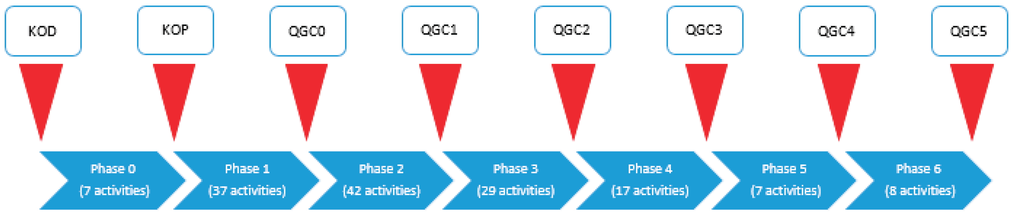
Figure 2.
Algorithm framework developed for scheduling projects with due dates to be respected.
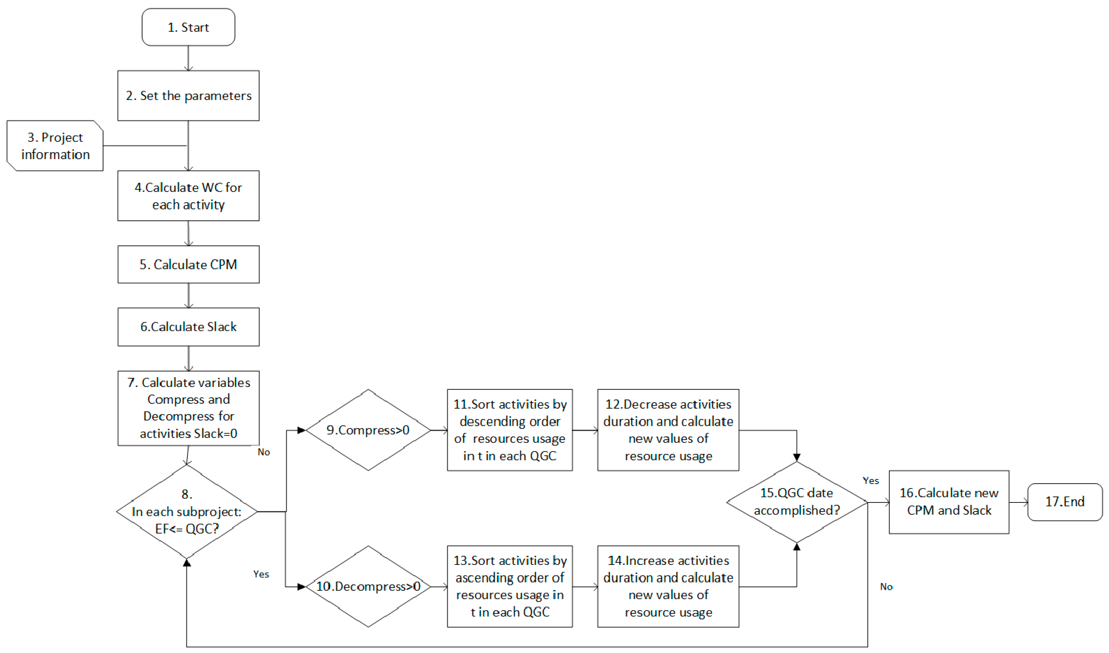
Figure 4.
Project distribution by Category.
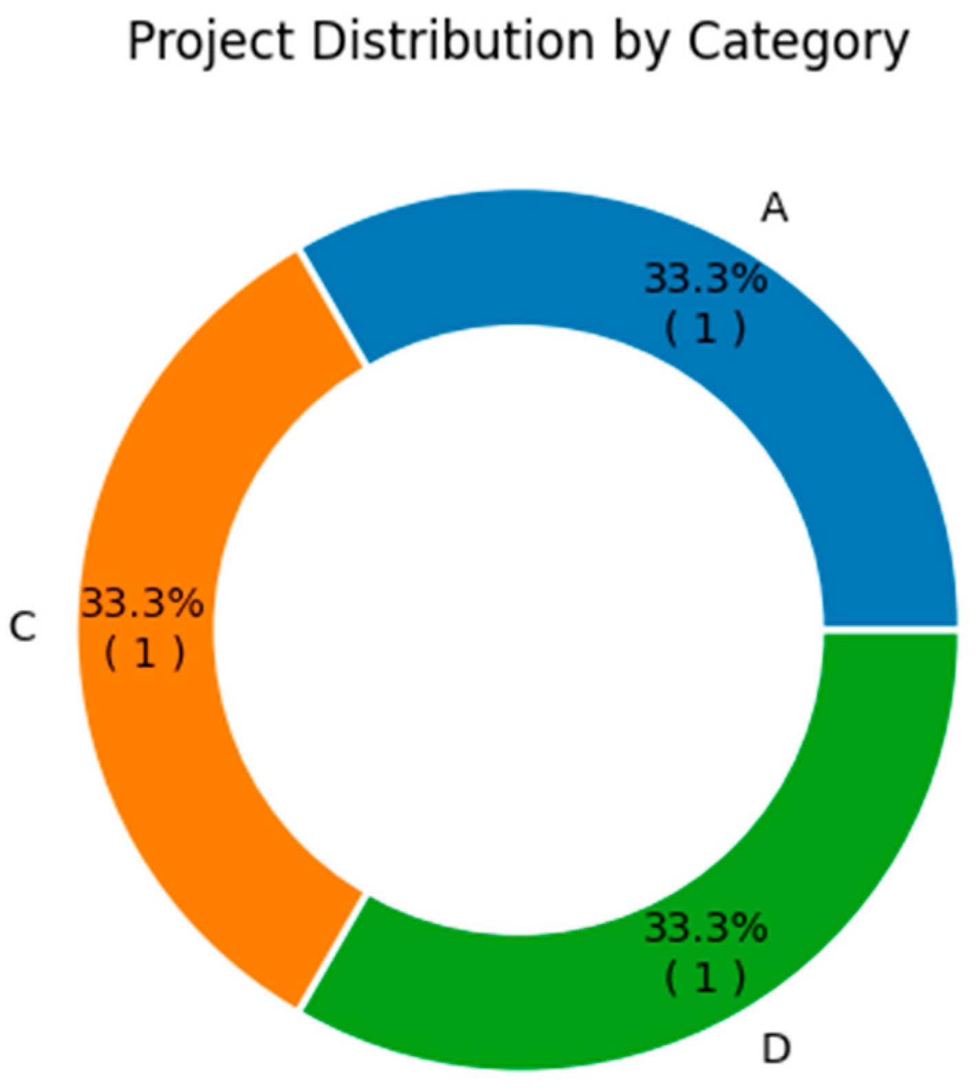
Figure 5.
Project distribution by iPM.
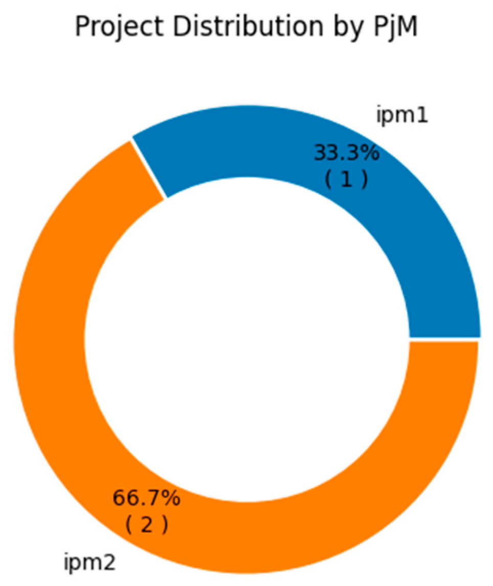
Figure 6.
Chart_by_iPM.
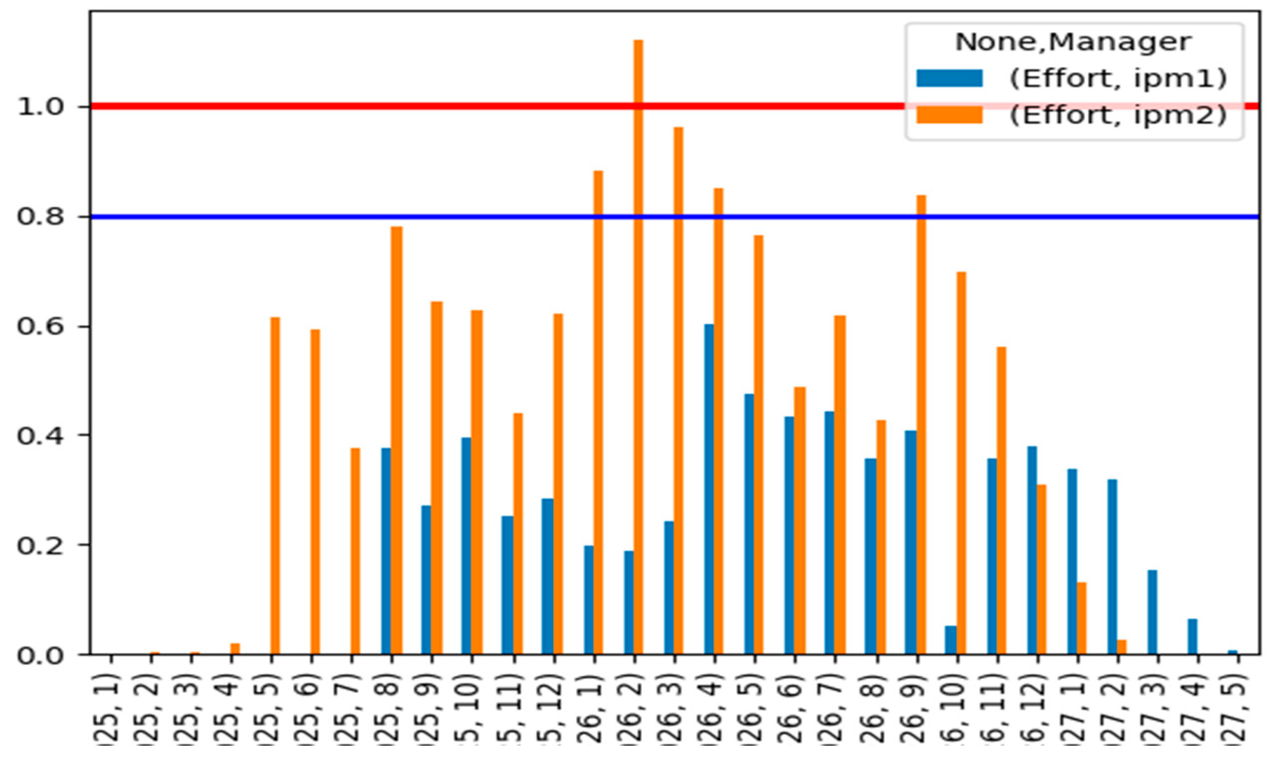
Figure 7.
Chart_by_Project.
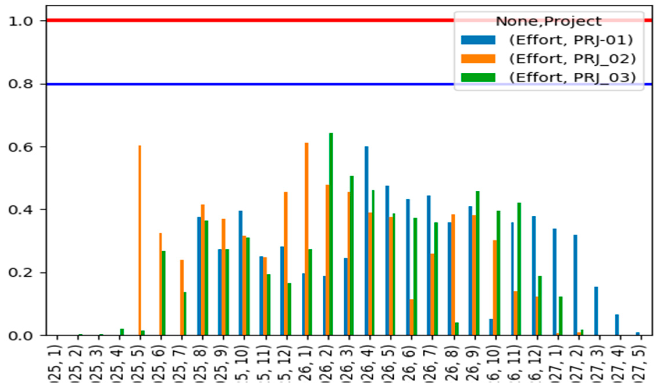
Table 1.
Input parameters of the developed model.
| Project characteristics | Project deliverables |
| Project ID | Start date of the project (KOD) |
| Project Name | Date of KOP |
| Project Type | Date of QGC0 |
| Project Category | Date of QGC1 |
| Project Sample | Date of QGC2 |
| Date of QGC3 | |
| Date of QGC4 |
Table 2.
Example of the input parameters.
| Input parameter | |
| Project ID | ID01 |
| Project Name | prj_01 |
| Project Type | Local industrialization |
| Project Category | A |
| Project Sample | ABCD |
| Start date of the project (KOD) | 2025/08/22 |
| Date of KOP | 2025/09/09 |
| Date of QGC0 | 2025/10/25 |
| Date of QGC1 | 2025/12/07 |
| Date of QGC2 | 2026/02/10 |
| Date of QGC3 | 2025/04/18 |
| Date of QGC4 | 2025/05/17 |
Table 3.
“Phase 0” start time for each project.
| Project name | prj01 | prj02 | prj03 |
| “Phase 0” start time | 2025-08-03 | 2025-05-22 | 2025-01-01 |
Table 4.
Representation of the critical path of phase 0.
| Act | Duration | Effort Man-hours | ES | EF | LS | LF | Slack | StartDate | EndDate | LS_Date | LF_Date |
| 1 | 1 | 0.060 | 0 | 1 | 0 | 1 | 0 | 2025-08-04 | 2025-08-05 | 2025-08-04 | 2025-08-05 |
| 2 | 1 | 0.250 | 1 | 2 | 1 | 2 | 0 | 2025-08-05 | 2025-08-06 | 2025-08-05 | 2025-08-06 |
| 3 | 1 | 0.375 | 2 | 3 | 5 | 6 | 3 | 2025-08-06 | 2025-08-07 | 2025-08-08 | 2025-08-12 |
| 4 | 1 | 0.130 | 2 | 3 | 2 | 3 | 0 | 2025-08-06 | 2025-08-07 | 2025-08-06 | 2025-08-07 |
| 5 | 3 | 0.130 | 3 | 6 | 3 | 6 | 0 | 2025-08-07 | 2025-08-12 | 2025-08-07 | 2025-08-12 |
| 6 | 1 | 0.190 | 2 | 3 | 4 | 5 | 2 | 2025-08-06 | 2025-08-07 | 2025-08-07 | 2025-08-08 |
| 7 | 1 | 0.043 | 3 | 4 | 5 | 6 | 2 | 2025-08-07 | 2025-08-08 | 2025-08-08 | 2025-08-12 |
Table 5.
Effort of activities.
| Act | Phase | Effort |
| 7 | 0 | 0.043 |
| 1 | 0 | 0.060 |
| 4 | 0 | 0.130 |
| 5 | 0 | 0.130 |
| 6 | 0 | 0.190 |
| 2 | 0 | 0.250 |
| 3 | 0 | 0.375 |
Table 6.
Prioritization of activities in ascending order by the minimum recorded value of resource use.
Table 6.
Prioritization of activities in ascending order by the minimum recorded value of resource use.
| Order | Activity | Minimum resource usage value |
| 1 | 1 | 0.06 |
| 2 | 4 | 0.13 |
| 3 | 5 | 0.13 |
| 4 | 2 | 0.25 |
Table 7.
Method for decreasing duration values for each activity.
| New activity duration values (days) | ||
| Ordered activities | Initial duration value (days) | Iteration 1 |
| 1 | 1 | 1 |
| 4 | 1 | 1 |
| 5 | 3 | 2 |
| 2 | 1 | 1 |
| Total subtracted | 0 | 1 |
| Total to subtract | 1 | 0 |
Table 8.
Adjustments to the resource usage rate after changing the activity duration.
| Activity | New values of |
| 1 | 0.060 |
| 2 | 0.250 |
| 4 | 0.130 |
| 5 | 0.195 |
Table 9.
Phase 0 network of activities updated with values adjusted to the new durations.
| Act | Duration | Effort –Man-hours | ES | EF | LS | LF | StartDate | EndDate | LS_Date | LF_Date |
| 1 | 0 | 0.060 | 0 | 0 | 0 | 0 | 2025-08-04 | 2025-08-04 | 2025-08-04 | 2025-08-04 |
| 2 | 1 | 0.250 | 0 | 1 | 0 | 1 | 2025-08-04 | 2025-08-05 | 2025-08-04 | 2025-08-05 |
| 3 | 1 | 0.375 | 1 | 2 | 1 | 2 | 2025-08-05 | 2025-08-06 | 2025-08-05 | 2025-08-06 |
| 4 | 1 | 0.130 | 2 | 3 | 4 | 5 | 2025-08-06 | 2025-08-07 | 2025-08-08 | 2025-08-11 |
| 5 | 1 | 0.195 | 2 | 3 | 2 | 3 | 2025-08-06 | 2025-08-07 | 2025-08-06 | 2025-08-07 |
| 6 | 2 | 0.190 | 3 | 5 | 3 | 5 | 2025-08-07 | 2025-08-11 | 2025-08-07 | 2025-08-11 |
| 7 | 1 | 0.043 | 2 | 3 | 3 | 4 | 2025-08-06 | 2025-08-07 | 2025-08-07 | 2025-08-08 |
Table 11.
Project_Pool worksheet overview.
| Effort | ||||
| Project | PRJ-01 | PRJ_02 | PRJ_03 | |
| Year | Month | |||
| 2025 | 1 | 0.000 | 0.000 | 0.001 |
| 2 | 0.000 | 0.000 | 0.002 | |
| 3 | 0.000 | 0.000 | 0.005 | |
| 4 | 0.000 | 0.000 | 0.020 | |
| 5 | 0.000 | 0.602 | 0.0135 | |
| 6 | 0.000 | 0.324 | 0.269 | |
| 7 | 0.000 | 0.240 | 0.136 | |
| 8 | 0.374 | 0.416 | 0.364 | |
| 9 | 0.272 | 0.369 | 0.273 | |
| 10 | 0.396 | 0.315 | 0.311 | |
| 11 | 0.251 | 0.247 | 0.193 | |
| 12 | 0.283 | 0.454 | 0.166 | |
| 2026 | 1 | 0.196 | 0.611 | 0.273 |
| 2 | 0.188 | 0.478 | 0.641 | |
| 3 | 0.243 | 0.454 | 0.506 | |
| 4 | 0.601 | 0.391 | 0.460 | |
| 5 | 0.474 | 0.376 | 0.387 | |
| 6 | 0.433 | 0.113 | 0.373 | |
| 7 | 0.443 | 0.260 | 0.357 | |
| 8 | 0.359 | 0.385 | 0.041 | |
| 9 | 0.408 | 0.381 | 0.458 | |
| 10 | 0.051 | 0.302 | 0.396 | |
| 11 | 0.358 | 0.139 | 0.421 | |
| 12 | 0.378 | 0.122 | 0.187 | |
| 2027 | 1 | 0.339 | 0.007 | 0.123 |
| 2 | 0.318 | 0.008 | 0.019 | |
| 3 | 0.153 | 0.000 | 0.000 | |
| 4 | 0.065 | 0.000 | 0.000 | |
| 5 | 0.008 | 0.000 | 0.000 | |
Table 12.
Manager_Pool overview.
| Effort | |||
| Manager | ipm1 | ipm2 | |
| Year | Month | ||
| 2025 | 1 | 0.000 | 0.001 |
| 2 | 0.000 | 0.002 | |
| 3 | 0.000 | 0.005 | |
| 4 | 0.000 | 0.020 | |
| 5 | 0.000 | 0.615 | |
| 6 | 0.000 | 0.593 | |
| 7 | 0.000 | 0.376 | |
| 8 | 0.374 | 0.780 | |
| 9 | 0.272 | 0.642 | |
| 10 | 0.396 | 0.626 | |
| 11 | 0.251 | 0.440 | |
| 12 | 0.283 | 0.620 | |
| 2026 | 1 | 0.196 | 0.883 |
| 2 | 0.188 | 1.120 | |
| 3 | 0.243 | 0.961 | |
| 4 | 0.601 | 0.851 | |
| 5 | 0.474 | 0.763 | |
| 6 | 0.433 | 0.487 | |
| 7 | 0.443 | 0.618 | |
| 8 | 0.358 | 0.426 | |
| 9 | 0.408 | 0.839 | |
| 10 | 0.051 | 0.699 | |
| 11 | 0.358 | 0.561 | |
| 12 | 0.378 | 0.309 | |
| 2027 | 1 | 0.339 | 0.130 |
| 2 | 0.318 | 0.027 | |
| 3 | 0.153 | 0.000 | |
| 4 | 0.065 | 0.000 | |
| 5 | 0.008 | 0.000 | |
Disclaimer/Publisher’s Note: The statements, opinions and data contained in all publications are solely those of the individual author(s) and contributor(s) and not of MDPI and/or the editor(s). MDPI and/or the editor(s) disclaim responsibility for any injury to people or property resulting from any ideas, methods, instructions or products referred to in the content. |
© 2025 by the authors. Licensee MDPI, Basel, Switzerland. This article is an open access article distributed under the terms and conditions of the Creative Commons Attribution (CC BY) license (http://creativecommons.org/licenses/by/4.0/).
Copyright: This open access article is published under a Creative Commons CC BY 4.0 license, which permit the free download, distribution, and reuse, provided that the author and preprint are cited in any reuse.


