Submitted:
24 July 2025
Posted:
25 July 2025
You are already at the latest version
Abstract
Thermoacoustic refrigerators offer a promising alternative to conventional refrigeration technologies because their unique operating principles pose no harm to the environment. This study focuses on key performance indicators (KPIs) for thermoacoustic refrigerators, relative to their performance efficiency. The coefficient of performance (COP), the Carnot coefficient of performance (COPC) and the coefficient of performance relative to Carnot’s COP (COPR), crucial KPIs, are analyzed within the framework of Carnot efficiency (temperature difference). By comparing the analyzed performance metrics of a thermoacoustic refrigerator, such as COP and COPR, for a case study, the analysis provides insights into areas for improvement and optimization. The results highlight the potential and limitations of the temperature difference in current thermoacoustic technologies and suggest pathways for enhancing their efficiency to meet or exceed traditional refrigeration benchmarks.
Keywords:
thermoacoustics
; design of experiments
; linear thermoacoustic theory
; COP
; COPC
; COPR
1. Introduction
The theoretical breakthrough in thermoacoustic refrigeration was developed by Nicklaus Rott [1] and represented an innovative approach to cooling technology, distinguished by its reliance on sound waves rather than conventional mechanical compressors. Since 1980, this method harnesses the power of acoustic waves to create temperature gradients, offering a potentially more efficient and environmentally friendly alternative to traditional refrigeration systems. Unlike standard refrigeration technologies that often rely on complex and energy-intensive processes, thermoacoustic refrigerators operate based on principles of thermodynamics and acoustics, which could lead to significant advancements in energy efficiency [2].
The main components of a thermoacoustic refrigerator are the resonator cavity, the stack, the acoustic driver and the heat exchangers, see Figure 1. The performance response depends primarily on the system’s design parameters, including operating conditions, the geometry of stack/regenerator, thermo-physical properties of the stack, working fluid, and acoustic driver [4,5].
Assessing the performance of thermoacoustic refrigerators is crucial for understanding their viability and areas for improvement. Key performance indicators (KPIs) such as the Coefficient of Performance (COP), the Carnot’s coefficient of performance (COPC) and the Carnot ratio of the COP (COPR) provide valuable insights to evaluate the effectiveness and efficiency of these systems. The COP measures the ratio of cooling power to input power, meanwhile, the COPC represents the theoretical maximum efficiency achievable by a refrigeration cycle operating between two thermal reservoirs, providing a benchmark against which real systems can be compared. The COPR offers a comparative perspective, illustrating the ratio of the actual COP to the COPC, thus highlighting the relative efficiency of the system. The relationship between the mentioned coefficients is defined by the internal energy U and the temperature difference and among reservoirs. Tijani [4,5] compared and showed, why the performance of standing-wave thermoacoustic devices falls below Carnot’s performance. To address this limitation, Tijani proposed incorporating two additional performance metrics: the COPC and the COPR.
By utilizing these three metrics—COP, COPC, and COPR—researchers can gain a more comprehensive understanding of thermoacoustic refrigerator performance. This triadic approach enables clearer insights into these systems’ efficiency and operational characteristics, facilitating better design decisions and optimizations. Tijani’s framework encourages a more rigorous assessment of performance metrics, ultimately contributing to advancements in the development and application of thermoacoustic refrigeration technology.
This study aims to evaluate these KPIs within the context of Carnot efficiency as well as to identify if the best obtained COP in [3] matches the COPC and COPR responses based on the same temperature difference. The evaluation is made based on the obtained results, where a case study was analyzed to determine the influence of the different parameters as well as their interaction on the COP response of a thermoacoustic device. Through this comparison, the research highlights both the potential benefits and limitations of thermoacoustic refrigeration, providing a pathway for optimizing these systems to meet or exceed traditional refrigeration standards.
2. Methods
2.1. Thermodynamics. Carnot Cycle for Refrigerators
A refrigerator works by transferring heat from a colder area (inside the fridge) to a warmer area (outside), which is the reverse of a heat engine, see Figure 2. The Carnot cycle can be applied to an idealized refrigerator to understand its maximum theoretical efficiency. A Carnot refrigerator operates in reverse compared to a Carnot heat engine. Instead of generating work by transferring heat from hot to cold, a refrigerator uses work to transfer heat from a cold reservoir (inside the refrigerator) to a hot reservoir (the surrounding environment). The key processes of the Carnot cycle, when applied to refrigeration (Figure 2), are: Isothermal compression (a-b): the refrigerant is compressed at the higher temperature releasing heat to the environment, adiabatic expansion (b-c): the refrigerant expands without heat exchange causing its temperature to decrease to , isothermal expansion (c-d): the refrigerant absorbs heat from the cold space (inside the fridge) at temperature , and adiabatic compression (d-a): the refrigerant is compressed again, raising its temperature back to .
The efficiency of a Carnot refrigerator depends only on the temperatures ( ) and () as follows,
where and are expressed in . In the Carnot cycle, , is the temperature at which heat is absorbed during the isothermal expansion process (from state a to b) in the left PV diagram, see Figure 2, whereas , is the temperature at which heat is rejected during the isothermal compression process. The greater the temperature difference between the reservoirs, the higher the efficiency, but the Carnot cycle represents the maximum theoretical efficiency that any refrigerator can achieve.
2.2. Key Performance Indicators (KPIs)
The efficiency of a thermoacoustic device is given by the ratio between the heat removed from the cold reservoir by unit of acoustic work input W, this ratio is known as Coefficient of Performance (COP), see Equation (2). The higher the COP, the more efficient the system. The exact mathematical expressions for and W can be found elsewhere [3,5].
The maximum possible efficiency of a refrigerator operating between two thermal reservoirs according to the Carnot cycle is represented by , see Equation (3). It is derived from the second Law of thermodynamics and provides an upper bound of efficiency of any real refrigerator.
The is given by the ratio between and , see Equation (4). It is often expressed as a percentage and indicates how efficiently the real system operates compared to the theoretical ideal. A distinctive feature of is that it weighs the value over the corresponding value of the temperature gradient.
2.3. Design of Experiments (DOE)
In a previous work [3] we combine the linear thermoacoustic theory (LTT) with the Design of Experiments (DOE) [6,7] methodology (also known as factorial design) to identify, control, and determine the critical parameters for enhancing the COP response. COP values were calculated using a script written in Python. The main idea was to quantify the contribution to the COP of each of the parameters on which it depends, as well as their interactions. It was shown that, for the analyzed study case (Figure 1), the COP depends on five dimensionless parameters shown in Table 1. The DOE incorporated all possible levels of a given number of factors within a specified range. These levels are categorized as “low” and “high”. Evaluating the sensibility of the COP parameters suggests that opting for the lower values rather than the upper ones can increase the COP to 1.76 within the interval given, using air as working gas at ambient temperature and pressure.
3. Results and Discussion
This research presents an interpretation based on the obtained COP results in [3] taking into consideration the other two KPI’s introduced in the above sections. It will show that by relying solely on the maximum COP estimation biased conclusions can be drawn.
To analyze these results in terms of the KPIs, their estimation is necessary based on their definitions, see Equations (3) and (4). However, it is first necessary to establish the values of and . Firstly, is the hot temperature, which in this case corresponds to the initial temperature of the refrigerator and is equal to the ambient temperature, . Secondly, corresponds to the cold temperature reached for a given configuration. For each configuration, there is a temperature gradient interval (column 4, Table 2), so the temperature can be calculated as . The result for each configuration is shown in column 8 of Table 2. With the previous clarifications, the COPC and COPR values can now be calculated for each configuration, using the previous definitions. The results are also shown in Table 2 (columns 9 and 10), and column 11 shows the percentage value of COPR.
The first interesting result observed from this comparison shown in Table 2 is that the highest COP values (Runs 1, 2, 11, 12) do not correspond to the highest COPR values (Runs 13 and 14). The second interesting result is that higher COPR values correspond to those where temperature gradients are larger, while higher COP values correspond to smaller gradients, see Figure 3. This clearly shows how maximizing the COP value can be biased while maximizing the COPR is more physically correct and its estimation allows adequate evaluation of the performance of these devices.
Based on the Table 2, the KPI metrics COP and COPR, along with various design factors, are graphically represented in Figure 3. Figure 3 illustrates the global impact of the analyzed parameters on the responses of the COPR and the COP [3]. As can be seen, with the exception of the temperature gradient, all parameters have the same trend. Other key insights for the main parameters can be summarized as follows:
-
COP Performance Analysis:
- High COP Values: Runs with the highest COP values include Run 1 and Run 2 (COP = 1.76), Run 11 and Run 12 (COP = 1.74). These configurations generally have lower spacing (), except Run 12 and lower values, indicating that reduced spacing and lower temperature difference enhance COP.
- Low COP Values: The lowest COP values, such as Run 7, Run 8 and Run 24 and (COP = 0.13), are associated with higher spacing (0.15), lower blocking ratios (0.25) and higher , suggesting that extreme values of these factors negatively impact performance. For these cases the impact of the length is minor.
-
Effect of the Blocking Ratio
- Lower Blocking Ratio: Low values of the blocking ratio (B = 0.25) tend to correlate with higher COP values (e.g., Run 1 and Run 2 with COP = 1.76). This indicates that a lowering blocking ratio might enhance the COP performance, by other hand the efficiency, represented by COPR, is not the highest (3%).
- High Blocking Ratio: Higher values of the blocking ratio (B = 0.75) generally result in higher COPR values. For example, Run 13 and Run 14 have some of the highest COPR values, suggesting better performance with a higher blocking ratio.
-
Temperature Gradient Impact ()
- Lower : Lower temperature gradients (e.g., 5 K) are associated with higher COP values and improved performance metrics, see Runs 1, 2, 9, 10, 11, and 12. However, Runs 13 and 14 with = 15 K show better COPC and COPR values compared to those with lower .
- Higher temperature gradients tend to improve the system’s thermodynamic efficiency, leading to higher COPR value, as shown by Run 14 (COPR = 4.9%), with a blocking ratio of 0.75 and a temperature difference of 15 K.
-
Length () Influence
- Shorter lengths ( m) tend to give higher COP values. Run 1 (COP = 1.76) and run 10 (COP = 1.28), which have shorter lengths, show higher efficiency compared to Runs with longer lengths of m. However, Run 14 shows the highest COPR = 4.9% with a shorter length.
- Longer Lengths ( = 0.15 m) are associated with a mix of higher and lower COP values depending on other factors. For example, Runs 1 and 2 have higher COP values (above 1.0) and lower COPR values (3.0 respectively) despite having shorter lengths, indicating that the effect of may be context-dependent.
-
Effectiveness of COPC and COPR
- Higher COPC values are typically observed with lower temperature For these cases the effect of the other parameters is minor.
- The Relative COP (COPR) values, which compare the actual system COP to the theoretical Carnot limit, show higher percentages for Runs with higher temperature gradients. This highlights that achieving closer-to-theoretical performance is easier when the temperature difference is maximized, as seen in Run 13 and Run 14.
-
Optimal Configuration
- High COP: Runs with configurations such as Runs 1 and 2 (COP = 1.76, = 0.05, = 5 K) exhibit the highest COP values.
- High COPC: Configurations with a higher mean temperature difference and smaller spacing, such as Runs 13 and 14 exhibit not the highest COPC values.
- High COPR: Runs with a higher mean temperature difference and smaller spacing generally yield higher COPR values. For instance, Run 13 and 14 have the highest COPR of 4.9.
-
Trade-offs Between Factors
- Spacing vs. Temperature Gradient: Reducing spacing () and increasing generally improve performance metrics. However, adjustments in spacing should be balanced with temperature gradient considerations to avoid performance drops.
- Temperature Gradient: Reducing to 5 K consistently improves COP performance across Runs, suggesting that this is one of the most important factors in improving system efficiency. However increasing to 15 K consistently improves COPR performance across Runs.
- Length of Stack (): Shorter stacks lead to higher COP and COPR values, indicating that reducing the length for heat transfer improves performance.
- Carnot Efficiency vs. Actual COP: The system performs closer to its theoretical limit when the temperature difference is maximized.
4. Conclusions
The system’s actual performance (COP) is considerably lower than the theoretical maximum (COPC) across all configurations. However, improving COPR (which measures how close the system is to the Carnot limit) involves optimizing parameters such as the temperature difference, stack length, and position. The best-performing configurations achieve COPR values of around 3-5%, suggesting room for substantial efficiency improvements.
Based on the insights, the design of a thermoacoustic refrigerator should focus on maximizing the temperature gradient (), reducing the length of the stack () and the spacing to improve COP, and maintaining a moderate blocking ratio (around 0.75). These factors, in combination, provide the highest COPR values and make the system more efficient relative to its theoretical performance.
Funding
This work was supported by CONAHCYT project 322615 (LaNITeF).
Acknowledgments
The authors would like to thank the "Laboratorio Nacional de Investigación en Tecnologías del Frío – LaNITeF". C.A. Escalante-Velázquez, would like to thank the CONAHCYT’s “Investigadoras e investigadores por México” program.
References
- Rott, N. , "Thermoacoustics" Advances in Applied Mechanics vol. 20, 1980.
- Kamil, M.Q.; Yahya, S.G.; Azzawi, I.D.J. Design methodology of standing-wave thermoacoustic refrigerator: theoretical analysis. Int. J. Air-Cond. Ref. 2023, 31, 7. [Google Scholar] [CrossRef]
- Peredo Fuentes, H.; Escalante Velazquez, C. A. Quantitative and Qualitative Analysis of Main Effects and Interaction Parameters in Thermoacoustic Refrigerators Performance. Preprints 2024, 2024090658. [Google Scholar] [CrossRef]
- Tijani MEH. Loudspeaker-driven thermo-acoustic refrigeration. Ph.D. thesis, unpublished, Eindhoven University of Technology, 2001.
- M.E.H Tijani, J.C. M.E.H Tijani, J.C.H Zeegers, A.T.A.M de Waele, Design of thermoacoustic refrigerators. Cryogenics 2002, 42, 49–57. [Google Scholar] [CrossRef]
- Montgomery, D.C. Design and analysis of experiments; John Wiley & Sons, 2000. [Google Scholar]
- Minitab 19 Statistical Software, 2010, Computer software, State Collage, PA:Minitab, Inc. www.minitab.com.
Figure 1.
Representative diagram of a standing-wave thermoacoustic refrigerator [3].
Figure 1.
Representative diagram of a standing-wave thermoacoustic refrigerator [3].
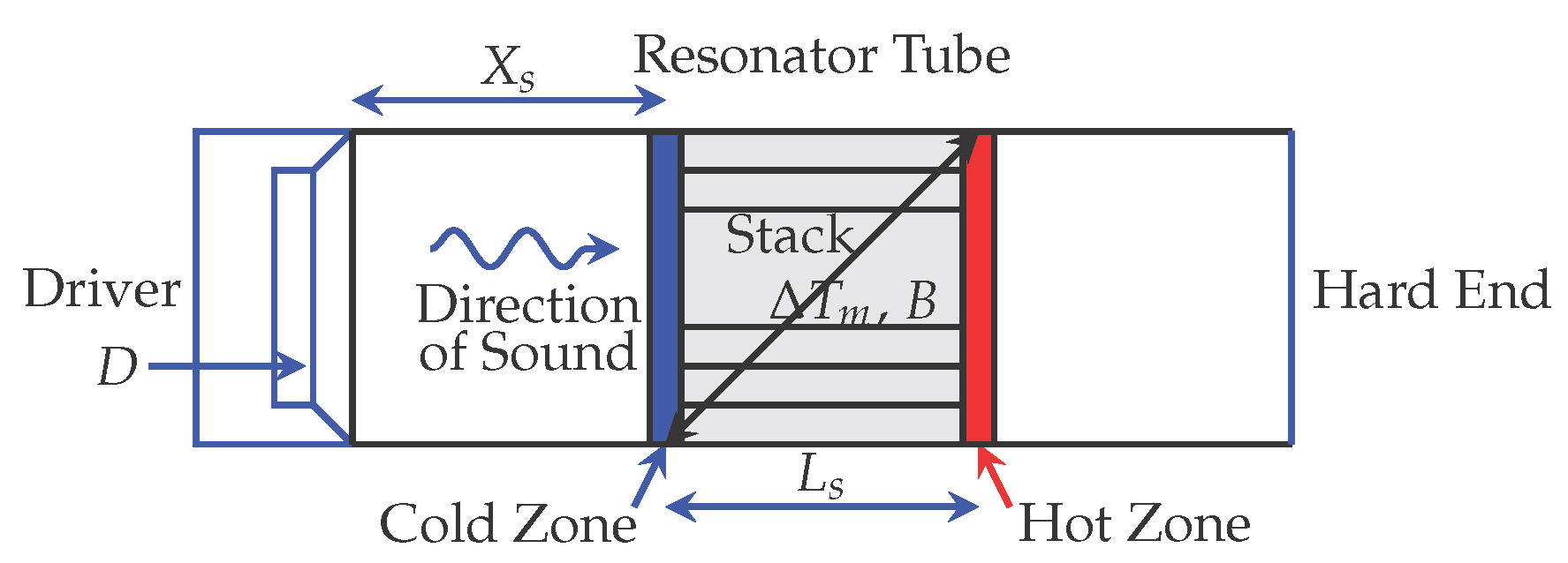
Figure 2.
Comparision Carnot’s cycle for a refrigerator (left) and engine (right).
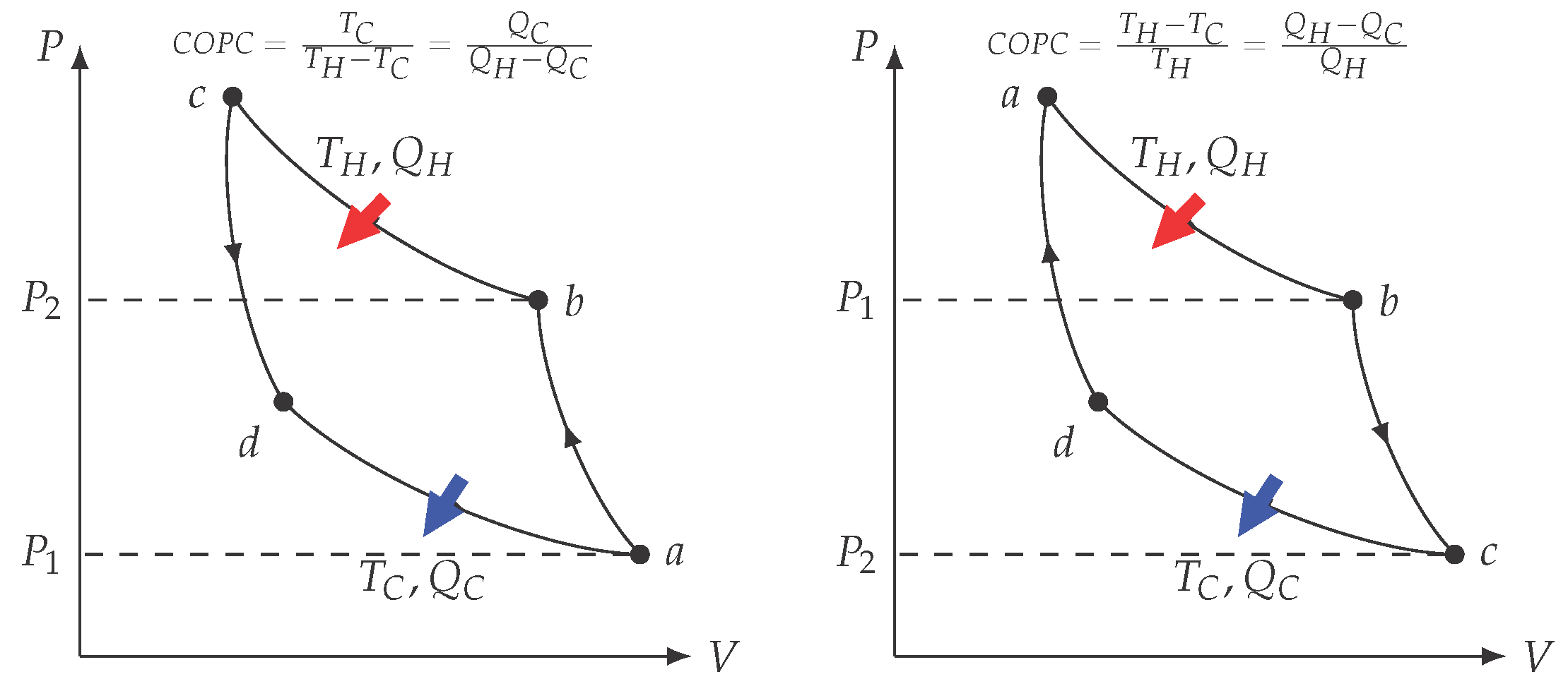
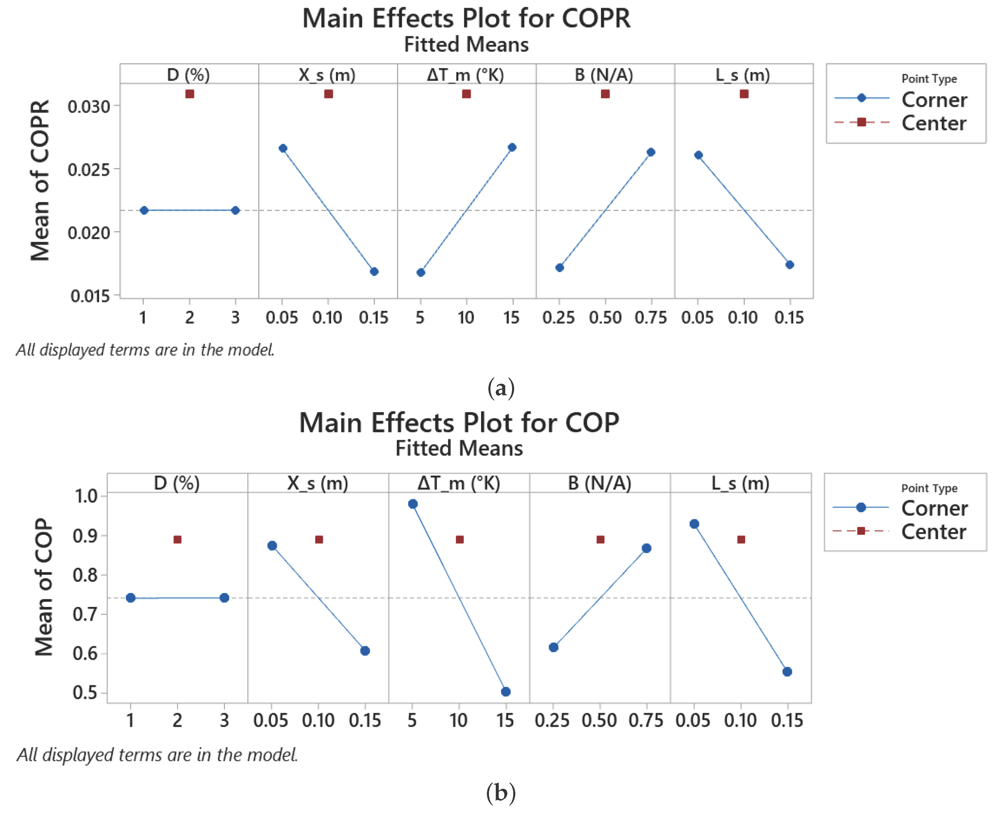
Figure 3.
Main Effects comparison. COPR’s Main Effects (a) and COP’s Main Effects (b) [3].

Table 1.
Levels and intervals by factor used in the DOE.
| Factor | Name | Level | Units |
| Low - High | |||
| A | Drive Ratio (D) | 1 3 | % |
| B | Stack Position () | 0.05 0.15 | m |
| C | Temperature () | 5 15 | °K |
| D | Blocking Ratio (B) | 0.25 0.75 | N/A |
| E | Regenerator length () | 0.05 0.15 | m |
Table 2.
Design of Experiments Orthogonal Array with dimensional parameters and COP responses in [3] with calculated , COPC and COPR responses.
Table 2.
Design of Experiments Orthogonal Array with dimensional parameters and COP responses in [3] with calculated , COPC and COPR responses.
| Factors | A | B | C | D | E | |||||
| Name | D | B | COP | COPC | COPR | COPR(%) | ||||
| Units | % | m | °K | N/A | m | °K | ||||
| Run | ||||||||||
| 15 | 1 | 0.15 | 15 | 0.75 | 0.05 | 0.59 | 283.15 | 18.87 | 0.0312 | 3.1 |
| 30 | 3 | 0.05 | 15 | 0.75 | 0.15 | 0.45 | 283.15 | 18.87 | 0.0238 | 2.4 |
| 25 | 1 | 0.05 | 5 | 0.75 | 0.15 | 0.48 | 293.15 | 58.63 | 0.0082 | 0.8 |
| 10 | 3 | 0.05 | 5 | 0.75 | 0.05 | 1.28 | 293.15 | 58.63 | 0.0218 | 2.2 |
| 16 | 3 | 0.15 | 15 | 0.75 | 0.05 | 0.59 | 283.15 | 18.87 | 0.0316 | 3.1 |
| 27 | 1 | 0.15 | 5 | 0.75 | 0.15 | 0.88 | 293.15 | 58.63 | 0.0150 | 1.5 |
| 3 | 1 | 0.15 | 5 | 0.25 | 0.05 | 0.40 | 293.15 | 58.63 | 0.0068 | 0.7 |
| 21 | 1 | 0.05 | 15 | 0.25 | 0.15 | 0.60 | 283.15 | 18.87 | 0.0318 | 3.2 |
| 19 | 1 | 0.15 | 5 | 0.25 | 0.15 | 0.40 | 293.15 | 58.63 | 0.0068 | 0.7 |
| 1 | 1 | 0.05 | 5 | 0.25 | 0.05 | 1.76 | 293.15 | 58.63 | 0.0300 | 3.0 |
| 11 | 1 | 0.15 | 5 | 0.75 | 0.05 | 1.74 | 293.15 | 58.63 | 0.0297 | 3.0 |
| 8 | 3 | 0.15 | 15 | 0.25 | 0.05 | 0.13 | 283.15 | 18.87 | 0.0069 | 0.7 |
| 26 | 3 | 0.05 | 5 | 0.75 | 0.15 | 0.49 | 293.15 | 58.63 | 0.0083 | 0.8 |
| 12 | 3 | 0.15 | 5 | 0.75 | 0.05 | 1.74 | 293.15 | 58.63 | 0.0297 | 3.0 |
| 13 | 1 | 0.05 | 15 | 0.75 | 0.05 | 0.93 | 283.15 | 18.87 | 0.0493 | 4.9 |
| 23 | 1 | 0.15 | 15 | 0.25 | 0.15 | 0.13 | 283.15 | 18.87 | 0.0069 | 0.7 |
| 29 | 1 | 0.05 | 15 | 0.75 | 0.15 | 0.45 | 283.15 | 18.87 | 0.0238 | 2.4 |
| 22 | 3 | 0.05 | 15 | 0.25 | 0.15 | 0.60 | 283.15 | 18.87 | 0.0318 | 3.2 |
| 28 | 3 | 0.15 | 5 | 0.75 | 0.15 | 0.89 | 293.15 | 58.63 | 0.0152 | 1.5 |
| 17 | 1 | 0.05 | 5 | 0.25 | 0.15 | 0.89 | 293.15 | 58.63 | 0.0152 | 1.5 |
| 4 | 3 | 0.15 | 5 | 0.25 | 0.05 | 0.40 | 293.15 | 58.63 | 0.0068 | 0.7 |
| 18 | 3 | 0.05 | 5 | 0.25 | 0.15 | 0.89 | 293.15 | 58.63 | 0.0152 | 1.5 |
| 14 | 3 | 0.05 | 15 | 0.75 | 0.05 | 0.93 | 283.15 | 18.87 | 0.0493 | 4.9 |
| 2 | 3 | 0.05 | 5 | 0.25 | 0.05 | 1.76 | 293.15 | 58.63 | 0.0300 | 3.0 |
| 6 | 3 | 0.05 | 15 | 0.25 | 0.05 | 0.61 | 283.15 | 18.87 | 0.0323 | 3.2 |
| 5 | 1 | 0.05 | 15 | 0.25 | 0.05 | 0.61 | 283.15 | 18.87 | 0.0323 | 3.2 |
| 32 | 3 | 0.15 | 15 | 0.75 | 0.15 | 0.58 | 283.15 | 18.87 | 0.0307 | 3.1 |
| 7 | 1 | 0.15 | 15 | 0.25 | 0.05 | 0.13 | 283.15 | 18.87 | 0.0069 | 0.7 |
| 33 | 2 | 0.10 | 10 | 0.50 | 0.10 | 0.89 | 288.15 | 28.82 | 0.0309 | 3.1 |
| 9 | 1 | 0.05 | 5 | 0.75 | 0.05 | 1.28 | 293.15 | 58.63 | 0.0218 | 2.1 |
| 20 | 3 | 0.15 | 5 | 0.25 | 0.15 | 0.40 | 293.15 | 58.63 | 0.0068 | 0.7 |
| 31 | 1 | 0.15 | 15 | 0.75 | 0.15 | 0.59 | 283.15 | 18.87 | 0.0313 | 3.1 |
| 24 | 3 | 0.15 | 15 | 0.25 | 0.15 | 0.13 | 283.15 | 18.87 | 0.0069 | 0.7 |
Disclaimer/Publisher’s Note: The statements, opinions and data contained in all publications are solely those of the individual author(s) and contributor(s) and not of MDPI and/or the editor(s). MDPI and/or the editor(s) disclaim responsibility for any injury to people or property resulting from any ideas, methods, instructions or products referred to in the content. |
© 2025 by the authors. Licensee MDPI, Basel, Switzerland. This article is an open access article distributed under the terms and conditions of the Creative Commons Attribution (CC BY) license (http://creativecommons.org/licenses/by/4.0/).
Copyright: This open access article is published under a Creative Commons CC BY 4.0 license, which permit the free download, distribution, and reuse, provided that the author and preprint are cited in any reuse.


