
Submitted:
23 July 2025
Posted:
24 July 2025
You are already at the latest version
Abstract
Accurate imputation of missing data in air quality monitoring is essential for reliable environmental assessment and modeling. This study compares two imputation methods, namely Random Forest (RF) and Bidirectional Recurrent Imputation for Time Series (BRITS), using data from the Mexico City Air Quality Monitoring Network (2014–2023). The analysis focuses on stations with less than 30% missingness and includes both pollutant (CO, NO, NO₂, NOₓ, SO₂, O₃, PM₁₀, PM₂.₅, PMCO) and meteorological (relative humidity, temperature, wind direction and speed) variables. Each station's data was split into 80% for training and 20% for validation, with 20% artificial missingness. Performance was assessed through two perspectives: local accuracy (MAE, RMSE) on masked subsets and distributional similarity on complete datasets (Two One-Sided Tests and Wasserstein Distance). RF achieved lower errors on masked subsets, whereas BRITS better preserved the complete distribution. Both methods struggled with highly variable features. On complete time series, BRITS produced more realistic imputations, while RF often generated extreme outliers. These findings demonstrate the advantages of deep learning for handling complex temporal dependencies and highlight the need for robust strategies for stations with extensive gaps. Enhancing the accuracy of imputations is crucial for improving forecasting, trend analysis, and public health decision-making.
Keywords:
air quality monitoring
; missing data imputation
; Bidirectional Recurrent Neural Networks (BRITS)
; Random Forest (RF)
; Mexico City Atmospheric Monitoring
1. Introduction
Air pollution refers to environmental contamination by any chemical, physical, or biological agent that modifies the natural characteristics of the atmosphere. It is primarily caused by motor vehicles, industrial activity, forest fires, and household combustion devices. Major air pollutants are particulate matter (PM₂.₅ and PM₁₀), carbon monoxide (CO), ozone (O3), nitrogen dioxide (NO2), and sulfur dioxide (SO2). Air pollution causes respiratory and cardiovascular diseases, among others, and is an important source of morbidity and mortality, shortening the average person’s lifespan by 1 year and 8 months (World Health Organization (WHO), 2024 [1]). According to the State of Global Air Report 2024 [2], air pollution accounted for more than 1 in 8 deaths globally in 2021 (8.1 million deaths), becoming the second risk factor for early death, surpassed only by high blood pressure. Over 700,000 deaths in children under five were associated with air pollution that year, representing 15% of all global deaths in this age group. Furthermore, air pollution is a major risk factor for death from heart disease, diabetes, lung cancer, and other noncommunicable diseases (State of Global Air (SoGA) [2]). The World Health Organization estimated that 99% of the global population breathes air exceeding its guideline limits, with the highest exposures in low- and middle-income countries. Since many air pollutants are also major contributors to greenhouse gas emissions, reducing air pollution offers dual benefits, improving public health and supporting climate change mitigation efforts (WHO Air pollution [3]).
Mexico City has a metropolitan area that exceeds 22 million inhabitants and has complex air pollution problems, caused primarily by heavy vehicular traffic, industrial emissions, extensive urbanization, and the burning of fossil fuels (Kim et al., 2021 [4], He et al., 2023 [5]).
This situation is aggravated by topographical factors that restrict atmospheric dispersion, because Mexico City sits over 2000 meters above sea level and is surrounded by mountains on three sides. These conditions result in naturally lower oxygen levels that contribute to incomplete fuel combustion and the accumulation of both primary and secondary pollutants, including fine particulate matter (PM2.5), ozone (O₃), and nitrogen dioxide (NO2). Although government initiatives (ProAire [6]) have led to improvements over the past decades, key pollutants continue to exceed guidelines at many monitoring stations across the city (He et al., 2023) [5]).
Effective air quality management relies on accurate environmental monitoring. Mexico City Atmospheric Monitoring System [6,7] operates a network of monitoring stations that collect hourly data on pollutant (CO: Carbon monoxide), NO: Nitric oxide, NO2: Nitrogen dioxide, NOₓ: Nitrogen oxides, NO + NO2, SO2: Sulfur dioxide, O3: Ozone, PM10, PM2.5, PMCO: coarse fraction: PM10–PM2.5) concentrations and meteorological (RH: relative humidity, Temp: Temperature, WDR: Wind Direction, WSP: Wind Speed) parameters to monitor air quality in real time.
However, missing data is a recurring issue, caused by sensor malfunctions, maintenance, power outages, and network transmission failures (Zhang & Zhou, 2024 [8]; Wang et al., 2023 [9]). These issues compromise the completeness and reliability of the dataset, obstructing subsequent analyses such as trend evaluation, forecasting, and epidemiological modeling (Hua et al., 2024 [10]). Imputing missing values in air quality time series is therefore essential to ensure data completeness and analytical robustness (Alkabbani et al., 2022 [11]).
While traditional imputation methods are limited in capturing the complex spatio-temporal dependencies inherent in environmental data, recent advances in machine and deep learning have opened promising avenues (see Table 1). Multiple strategies have been developed to handle missing data in atmospheric monitoring systems. Traditional methods, such as mean/median substitution or linear interpolation, are simple but often fail in complex, multivariate contexts with non-linear dependencies or temporal structure (Wang et al., 2023 [9]). More advanced statistical approaches like Multivariate Imputation by Chained Equations (MICE) and regression-based methods offer improvements but are sensitive to assumptions about data distributions (Hua et al., 2024 [10]).
Machine learning techniques, including k-nearest neighbors (KNN), support vector regression (SVR), and decision trees, have shown enhanced accuracy, especially when capturing local or spatial patterns (Zhang & Zhou, 2024 [8], Wang et al., 2023 [9], Hua et al., 2024 [10]; Camastra et al. 2022 [12]). Hybrid and ensemble models have also emerged to better exploit spatial-temporal correlations (He et al. (2023) [5], Wang et al. (2023) [9]).
In recent years, deep learning has become central to missing data imputation in air quality research. RNN-based models such as Gated Recurrent Unit-Decay (GRU-D)( Che et al., 2018 [13]) and Bidirectional Recurrent Imputation for Time Series (BRITS) ( Cao et al., 2018 [14]) leverage temporal dependencies and trainable masking strategies, significantly improving performance on time series with irregular missingness. Similarly, generative models have been applied for their ability to more realistically reconstruct missing values. Among them, Generative Adversarial Imputation Nets (GAIN) ( Yoon et al., 2018 [15]) introduces adversarial training into the imputation task, improving robustness across diverse datasets. A recent review by Shahbazian and Greco (2023) [16] presents an extensive survey of several imputation methods based on Generative Adversarial Networks (GAN), covering applications in healthcare, finance, meteorology, and air quality. The review highlights the strengths of these models in preserving statistical distributions and generating more realistic imputations compared to traditional techniques. Other novel architectures have also been proposed, such as Graph Recurrent Imputation Network (GRIN) (Cini et al. 2021 [17]), a graph neural network imputation method, and Self-Attention-Based Imputation for Time Series (SAITS) (Du et al. 2023 [18]), a transformer-based model, which further expands the tools for handling missing data in structured environmental datasets.
Recent studies have explored the use of advanced machine and deep learning models to address missing data in air quality monitoring and to improve forecasting accuracy. A brief literature review of recent studies on air quality data imputation and prediction is presented below. Table 1 summarizes the key contributions in the field, with a focus on datasets, modeling techniques, study targets, and main findings.
Colorado Cifuentes & Flores Tlacuahua (2021) [19] proposed a deep learning approach for short-term air pollution forecasting in Monterrey, Mexico, using hourly data (2012–2017) of eight pollutants and seven meteorological variables from 13 monitoring stations. Seasonal decomposition was applied to impute missing values, and a feedforward Deep Neural Network (DNN) was trained to predict O₃, PM₂.₅, and PM₁₀ concentrations up to 24 hours in advance. A key limitation identified was the reduced accuracy of the model in predicting extreme pollution events.
Kim et al. (2021) [3] developed an interpretable deep learning model based on the Neural Basis Expansion Analysis for interpretable Time Series (N-BEATS) architecture to impute minute-level PM₂.₅ and PM₁₀ concentrations using data from 24 stations in Guro-gu and 42 stations in Dangjin-si, South Korea. Real missingness rates of 7.91% and 16.1% were reported, with an additional 20% of data artificially removed for testing. N-BEATS outperformed baseline techniques (mean, spatial average, MICE) and enabled interpretability through trend, seasonality, and residual components. However, it showed limitations in capturing long-term seasonal trends due to the use of fixed-period Fourier components.
Alahamade & Lake (2021) [20] evaluated six imputation strategies using hourly pollutant data (PM₁₀, PM₂.₅, O₃, NO₂) from the UK’s Automatic Urban and Rural Network (AURN) for the period 2015–2017. Their approach involved three groups of models: (1) clustering-based (CA: cluster average, CA+ENV: average within same station type, CA+REG: average within same region) using multivariate time series (MVTS) to group stations by temporal similarity; (2) spatial proximity-based (1NN: nearest station; 2NN: two nearest stations); and (3) ensemble: median of outputs of all five methods. The ensemble model performed best for O₃, PM₁₀, and PM₂.₅, while CA+ENV outperformed others for NO₂ due to its high spatial variability. Performance depended on pollutant and station type, and extreme values were slightly under- or overestimated.
He et al. (2023) [5] developed a predictive modeling framework for daily NO₂ concentrations in Mexico City by integrating ground-based (RAMA: Air quality monitoring network in Mexico City), satellite observations (OMI: Ozone Monitoring Instrument, and TROPOMI: TROPOspheric Monitoring Instrument), and meteorological data (CAMS: Copernicus Atmosphere Monitoring Service). Missing values were imputed using the MissForest algorithm. Random Forest and XGBoost outperformed the Generalized Additive Model (GAM), demonstrating the value of hybrid data sources for spatial-temporal NO₂ estimation.
Wang et al. (2023) [9] developed BRITS-ALSTM, a hybrid deep learning model that integrates BRITS with an attention-based Long Short-Term Memory (LSTM) decoder. The model was applied to hourly air quality data (2019–2022) from 16 monitoring stations in the alpine regions of China, covering six pollutants (PM₂.₅, PM₁₀, O₃, NO₂, SO₂, and CO). Both real missingness (5%–22%) and artificial gaps (30%) were considered. BRITS-ALSTM consistently outperformed classical and deep learning baselines, showing strong performance across pollutants and various missing data patterns.
Zhang and Zhou (2024) [8] proposed TMLSTM-AE, a hybrid deep learning model that combines LSTM, autoencoder architecture, and transfer learning to impute missing values in the PM2.5 time series from Xi’an, China, characterized by single, block, and long-interval missing patterns. Artificial missingness ranging from 10% to 50% was introduced to evaluate performance. TMLSTM-AE was compared with both classical and deep learning approaches. TMLSTM-AE outperformed all baselines, especially in scenarios with long and consecutive missing gaps, demonstrating its capacity to capture spatio-temporal dependencies.
Hua et al. (2024) [10] evaluated several traditional imputation methods (mean, median, k-Nearest Neighbor Imputation (KNNI), and MICE) and deep learning models (SAITS, BRITS, MRNN, and Transformer) using six real-world air quality datasets from Germany, China, Taiwan, and Vietnam. The study introduced artificial missingness ranging from 10% to 80%. Results showed that SAITS and BRITS achieved the lowest imputation errors, while KNN performed well on large datasets with high missing rates (up to 80%). In contrast, MICE was more effective on smaller datasets but incurred higher computational costs. The Transformer-based model underperformed across most scenarios. The authors concluded that no single method is universally optimal; performance depends on dataset size, missingness rate, and application context.
As summarized in this analysis (Table 1), recent studies have increasingly adopted deep learning techniques, such as RNNs, attention-based models, and hybrid architectures, for imputing air quality data, particularly under complex and irregular missingness patterns.
BRITS has demonstrated high performance in reconstructing missing values in multivariate and temporally structured data, using bidirectional recurrent neural networks and a learnable masking mechanism. While some studies in Mexico have explored statistical and machine learning approaches for air quality prediction, the application of deep learning-based imputation remains limited. Conversely, tree-based ensemble methods such as Random Forest have been widely used for imputation in environmental datasets due to their flexibility and ability to handle nonlinear relationships, although they do not explicitly model temporal structure.
The objective of this study is to compare the performance of BRITS, a state-of-the-art deep learning model, with Random Forest, a robust machine learning baseline, for imputing missing hourly observations in air quality time series from Mexico City, considering multiple pollutants (CO, NO, NO₂, NOₓ, SO₂, O₃, PM₁₀, PM₂.₅, PMCO) and meteorological variables (RH, TMP, WDR, WSP). This study aims to identify the strengths and limitations of each approach and to contribute to the development of more accurate and reliable strategies for environmental data imputation.
2. Materials and Methods
2.1. Database
2.1.1. Study Area
Mexico City, the capital and largest metropolitan area in Mexico, is located at over 2,000 meters above sea level and is surrounded by mountains on three sides. In 2020, this city had a population of approximately 9.2 million, while the Valley of Mexico Metropolitan Area had 21.8 million inhabitants, with projections estimating 22.75 million by 2025 [21]. The Valley of Mexico Metropolitan Area includes Mexico City and its adjacent suburban areas. The city covers an area of 1,494.3 km² and faces persistent air quality challenges due to its topography, urban density, and emission sources.
2.1.2. Data Collection and Integration
This study uses hourly data from the Mexico City Atmospheric Monitoring Network (Red Automática de Monitoreo Atmosférico, RAMA [7]), comprising air pollutants (PM₂.₅, PM₁₀, NO, NO₂, NOₓ, SO₂, CO, and O₃) and meteorological variables (temperature, relative humidity, wind speed and wind direction). Data were collected from January 1, 2014, to December 31, 2023, including both dry and rainy seasons.
Annual files for each variable were loaded, concatenated, and transformed into a long format with standardized columns. Date and hour were combined into a single datetime column. All variables were then merged into a unified multivariate time series, aligned by monitoring station and timestamp. Missing values originally coded as -99 were replaced with NaN.
2.1.3. Missing Data Patterns Analysis and Station Filtering
A comprehensive analysis of the percentage of missing data per variable and monitoring station revealed several significant patterns. While some stations exhibit relatively low missingness across all variables, many show critical data quality issues. Several stations, including LAA, COY, and TPN, have complete (100%) missing data for most variables, making them unsuitable for time series modeling.
Additionally, PMCO, PM₂.₅, and PM₁₀ consistently have 100% missing values across many stations. In contrast, pollutants such as CO, NO₂, and O₃ generally exhibit lower percentages of missing data across a wider range of stations, indicating relatively higher data availability. Figure 1 shows a heatmap of the missing data percentages for all monitoring stations included in the dataset. Variables with more than 30% missing data are highlighted in red.
Due to the high proportion of missing values across many stations, a missingness threshold was used to select the stations included in the imputation procedure. Only stations with at least 70% of observed data for each variable were selected. Figure 2 shows the RAMA monitoring network, with the selected stations highlighted in blue. Some variables were excluded from the selected stations when they exceeded the missing data threshold, for example PM₁₀ at NEZ station and PMCO, PM₂.₅, and PM₁₀ at UAX, FAC, and NEX stations, which had complete 100% missing values.
2.1.4. Missing Data Patterns in Selected Monitoring Station
Figure 3 shows the total percentage of missing values per variable for each of the 10 selected monitoring stations (CUA, FAC, MER, MGH, NEZ, PED, SAG, TLA, UAX, VIF). The missingness rates vary across stations and variables ( i.e., some stations have more missing data than others, and within each station, certain variables (e.g., PM₁₀, PM₂.₅, and PMCO) may exhibit particularly high or complete missingness). Although most of these stations have less than 20% missing data overall, certain variables such as PM₁₀, PM₂.₅, and PMCO, show very high or complete absence of data in some stations. For this first stage of the imputation project, only the best-informed stations were selected to ensure the quality of imputed values.
To better understand the temporal structure of missingness, nullity matrices were generated for each station. As illustrated in Figure 4, these visualizations reveal prolonged gaps in data across multiple variables, suggesting that the missing values are not randomly distributed but may be associated with systematic sensor failures.
2.2. Model Training and Evaluation Pipeline
- Missing data identification: Binary masks were created to identify real missing values in the dataset.
- Data splitting: Each station’s dataset was divided into 80% for training and 20% for testing.
- Hyperparameter optimization: Hyperparameter tuning was performed in sequential steps due to computational constraints.
- Artificial missingness for evaluation: To enable controlled performance assessment, 20% of the observed values in the test set were randomly removed under a Missing Completely At Random (MCAR) assumption. This masking allowed direct comparison between imputed and ground-truth values.
- Normalization: For the BRITS method, all variables were standardized using MinMaxScaler normalization, applied separately to the training and test datasets.
- Model Training and Evaluation: After hyperparameters optimization, models were retrained using the full training set and evaluated on the masked test set. Imputation performance was assessed using several evaluation metrics including MAE, RMSE, Wasserstein Distance, and TOST equivalence tests.
2.3. Model Training
To assess imputation quality across different methodological paradigms, two models were implemented: a classical machine learning method (Random Forest) and a deep learning model (BRITS). These models provide contrasting approaches to reconstructing missing environmental data, ranging from ensemble-based predictions to recurrent architectures that can model temporal dependencies.
2.3.1. Random Forest (RF) Hyperparameter Optimization
The Random Forest Regressor offers a robust and interpretable solution for multivariate imputation. We used IterativeImputer from scikit-learn with a Random Forest estimator to iteratively predict missing values using the available features at each timestamp. This approach can model complex nonlinear dependencies and often achieves high accuracy.
Hyperparameter tuning was performed manually using a staged grid search, due to computational constraints. This process used five steps to optimize one hyperparameter at a time:
- n_estimators: Number of trees in the ensemble.
- max_depth: Maximum depth of individual trees.
- max_iter: Number of iterations in the iterative imputation process (specific to IterativeImputer).
- min_samples_split: Minimum number of samples required to split an internal node.
- min_samples_leaf: Minimum number of samples required to be at a leaf node.
The default values and evaluated ranges for these hyperparameters are presented in Table 2, section (a).
2.3.2. BRITS Hyperparameter Optimization
BRITS is a deep learning model designed specifically for imputation data in multivariate time series, without relying on linear dynamics or strong prior assumptions. It is based on a bidirectional recurrent architecture that processes time series data in both forward and backward directions using Recurrent Neural Networks (RNNs), allowing the model to learn temporal dependencies from both past and future contexts (Cao et al. [14]).
Unlike traditional methods such as MICE, where missing values are pre-filled and treated as known inputs, BRITS treats missing values as latent variables embedded within the model’s computation graph. These are dynamically updated through backpropagation during training, enabling more accurate and context-aware imputations. As reported by Hua et al. [10], BRITS has shown strong performance on air quality datasets by effectively capturing nonlinear and correlated missing patterns.
Hyperparameter tuning was carried out manually in three sequential stages using a grid search strategy. In each stage, a subset of parameters was optimized while others were fixed:
- Stage 1: RNN units and subsequence length were tuned, with learning rate = 0.005, batch size = 64, use_regularization = False, and dropout_rate = 0.2 held constant.
- Stage 2: learning rate and batch size were tuned, keeping use_regularization = False and dropout_rate = 0.2 fixed.
- Stage 3: use_regularization and dropout_rate were jointly optimized.
Brief descriptions:
- RNN units: Number of hidden units in the RNN layers. Higher values improve model capacity to learn temporal patterns.
- subsequence length: Input window size used during training.
- learning rate: Controls the optimizer’s step size.
- batch size: Number of samples per training batch.
- use_regularization: Whether to apply dropout/L2 to prevent overfitting.
- dropout_rate: Proportion of neurons randomly deactivated during training.
The default values and evaluated ranges for these hyperparameters are presented in Table 2, section (b).
After hyperparameter tuning, the final model for each station was trained using 80% of the data and the corresponding optimal hyperparameter values. Model performance was then evaluated on the remaining 20% test set. To assess imputation accuracy, a mask was applied to randomly hide 20% of the observed values within the test set, simulating missing data. The model’s imputations were compared against these masked ground-truth values to compute the evaluation metrics.
2.4. Model Evaluation
To evaluate the imputation performance, four metrics were used: Mean Absolute Error (MAE), Root Mean Squared Error (RMSE), Two One-Sided Tests (TOST) AND Wasserstein Distance.
- Mean Absolute Error (MAE) quantifies the average absolute difference between imputed values ŷₜ and observed values yₜ:
Where is the number of data points.
- 2.
- Root Mean Squared Error (RMSE) measures the square root of the average squared differences between imputed and observed values:
- 3.
- Wasserstein Distance, also known as Earth Mover’s Distance (EMD), measures the dissimilarity between two probability distributions by calculating the minimum effort required to transform one distribution into another [23]. In the context of air quality time series, it is useful for comparing distributions of imputed and observed values. Given two cumulative distribution functions, and , the first-order Wasserstein distance is defined as:
- 4.
- The Two One-Sided Test (TOST [22]) is a statistical procedure used to assess the equivalence between the mean of imputed and observed values. Unlike conventional statistical tests that seek to detect significant differences, TOST is specifically designed to demonstrate equivalence, that is, to confirm that the difference is small enough to be considered negligible within a predefined tolerance margin. Let μₒ and μᵢ be the means of observed and imputed values, respectively. According to Santamaría-Bonfil et al. [2], TOST is implemented as two one-sided t-tests:
where Δ is a defined equivalence margin. Equivalence is declared only if both null hypotheses are rejected, confirming that the mean difference lies entirely within the interval (). This criterion ensures that the imputed values do not statistically differ from the observed values beyond an acceptable tolerance. In this study, we used a significance level α = 0.05, and equivalence margins based on ±10% of the observed mean.
3. Results
3.1. Results of Hyperparameter Optimization
Hyperparameter tuning was performed in sequential steps as described in section 2.3 “Model Training”. For Random Forest, hyperparameter tuning revealed notable variability across stations (Table 3). The number of estimators (n_estimators) ranged from 10 to 50, while the maximum tree depth (max_depth) was commonly set to 10 or 20, though some cases used no depth limit. The number of imputation iterations (max_iter) varied from 5 to 20, and the minimum samples required to split a node (min_samples_split) and to remain at a leaf node (min_samples_leaf) showed diverse configurations, indicating sensitivity to local data structure. Overall, smaller leaf sizes (1 to 6) and moderate (2 to 15) split thresholds were preferred.
The optimized hyperparameters suggest that stations with more complex patterns (e.g., PED, SAG) required deeper trees (max_depth = 20) and more estimators (50), while others (e.g., CUA, VIF, MGH) performed better with shallower models (max_depth = 10) and fewer estimators (10–20). Variations in min_samples_split and min_samples_leaf also suggest differences in noise levels and local dynamics across stations.
For BRITS, optimal hyperparameter settings were more consistent (Table 4). A large hidden dimension was generally preferred, with 512 RNN units for most stations. Subsequence length values commonly ranged from 32 to 64, and the learning rate was predominantly fixed at 0.005. The batch size was mostly set to 32, indicating a trade-off between stability and speed. Regularization was selectively applied, and dropout was commonly set to 0.2, except for a few cases where 0.1 or 0.3 yielded better results.
BRITS showed consistent optimal settings across stations, favoring large hidden layers and moderate subsequence lengths, whereas Random Forest required highly station-specific configurations, reflecting its adaptability to local variability but also its sensitivity to irregular missingness patterns.
3.2. Results of Imputation Models
After hyperparameter optimization, the final models were retrained on the full 80% training set using the selected optimal hyperparameter configurations. Evaluation was performed on the 20% test set. Additionally, to simulate realistic missingness and allow controlled performance evaluation, 20% of the observed values in the test set were randomly masked. The imputed values were compared to these hidden ground-truth values using four metrics: Mean Absolute Error (MAE), Root Mean Squared Error (RMSE) on masked subsets, and Wasserstein Distance and TOST for equivalence testing on complete distributions.
3.2.1. Performance Evaluation on Masked Subset
MAE and RMSE metrics were computed using 20% of observed values randomly masked from the validation set.
MAE Results
Figure 5, Figure 6 and Figure 7 show the distribution of imputation errors, expressed as MAE and RMSE, for all variables across the ten stations, comparing RF and BRITS models. Each subplot corresponds to a specific variable with its original scale, because these metrics are reported in the original units of each variable and must be compared only within the same context.
Figure 5 presents MAE results for RF and BRITS across all stations within each variable. RF consistently achieved lower MAE values than BRITS for every variable. The largest differences occurred in reactive gases such as NO, NO₂, and NOx, where RF errors were less than half those of BRITS. For example, in station MER, the MAE for NOx was 8.66 with RF versus 26.62 with BRITS, while in TLA, PM10 showed 4.85 for RF compared to 18.14 for BRITS (Table A1).
RMSE Results
Figure 6 shows a similar trend for RMSE. RF had smaller imputation errors and lower dispersion across stations compared to BRITS. RMSE differences were particularly notable for pollutants with high variability, such as NO, NOx, and PM10. For example, in station MER, RF achieved an RMSE of 20.36 for NOx, while BRITS reached 38.50; in TLA, PM10 showed 10.77 versus 24.25, respectively. Because RMSE penalizes large deviations quadratically, these higher values for BRITS suggest greater sensitivity to extreme imputation errors compared to RF.
3.2.2. Distributional Similarity Assessment
Wasserstein Distance and TOST were applied to the complete distribution of each variable, comparing the original dataset with the imputed dataset. These complete distributions showed a different trend than the masked subset.
Results of Wasserstein Distance
BRITS achieved lower Wasserstein Distance values than RF for most variables, indicating superior preservation of the original data statistical distribution (Figure 7). For example, in station MER, NOx had 0.80 for RF compared to 0.40 for BRITS, and in station TLA, PM2.5 showed 0.95 for RF versus 0.45 for BRITS. Similarly, in station SAG, NO₂ presented 1.35 with RF versus 0.64 with BRITS, and in CUA, NO₂ was 1.22 for RF against 0.59 for BRITS. BRITS also exhibited lower variability across stations, reflecting more consistent alignment with the true distributions. RF, despite achieving the best local accuracy (MAE and RMSE), displayed higher Wasserstein Distance values in many cases, underscoring a trade-off between decreasing individual errors and preserving the complete statistical distribution.
Results of TOST
Figure 8 presents a comparison between original means, imputed means, and TOST equivalence limits for each variable and station. In all cases the TOST equivalence criterion was satisfied, indicating that the imputed means were statistically equivalent to the original means within the predefined tolerance. Each subplot corresponds to a specific variable, while each row within a subplot represents one station. Black open circles indicate the observed mean for the complete dataset, while blue and red open circles represent the means obtained from the RF and BRITS imputation models, respectively. Horizontal dashed lines indicate the TOST equivalence bounds, defined as ±5% of the original mean for each variable. These bounds represent the range within which the imputed mean would be considered statistically equivalent to the original mean. This visualization facilitates a clear assessment of the proximity of the imputed means to the observed mean across variables and stations.
The comparison of differences between observed and imputed means across stations reveals several patterns in the performance of RF and BRITS. Overall, most differences remained small (< ±1 unit), indicating that both models achieved high accuracy for most variables. However, BRITS showed a slight overestimation tendency for several pollutants, particularly for NO, NOx, PM10, and PM2.5. While RF generally was stable, it exhibited higher variability in some cases, with both negative and positive deviations, especially in variables with greater heterogeneity, such as wind direction (WDR).
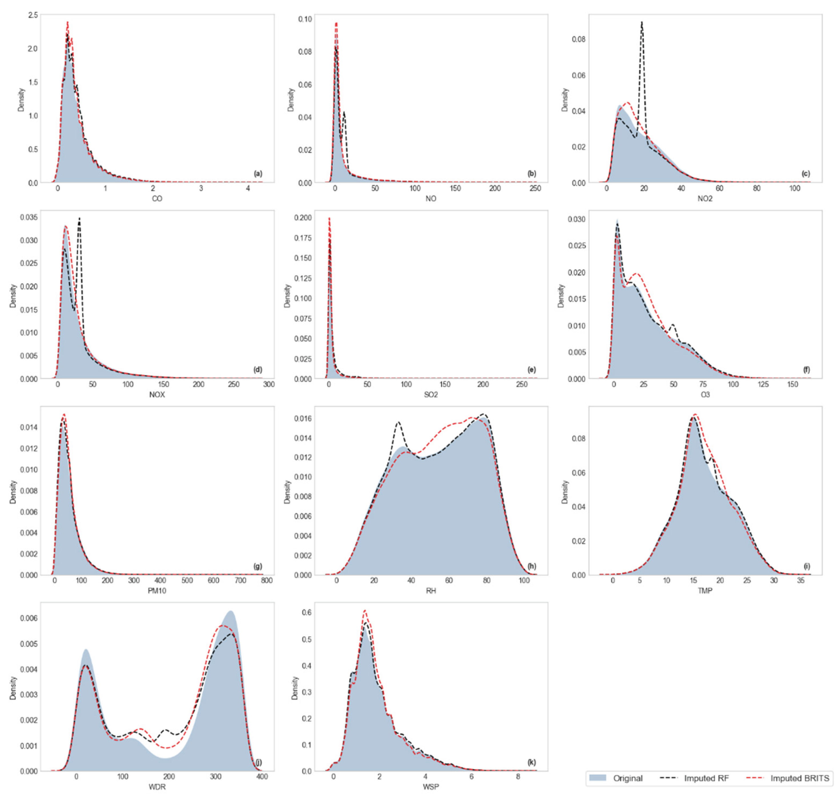
Visualization of Kernel Density Estimation (KDE)
KDE is a technique used to estimate the probability distribution of a dataset in a smooth and continuous manner. It is widely applied in exploratory analysis to examine the shape of the distribution (e.g., symmetric, skewed, multimodal). In visualization, a KDE plot is a curve that represents the estimated density derived from the data.
Figure 9 shows KDE-based estimated distributions for the MER station, comparing original data (shaded area) with imputations from RF (black dashed line) and BRITS (red dashed line). Overall, both techniques adequately captured the global shape of the original distributions. However, notable differences are observed for variables with high skewness or multimodality. For pollutants such as CO, NO, NO₂, and NOx (Figure 9 a–d), the imputed distributions closely followed the right-skewed pattern of these variables, although RF tended to generate sharper peaks around central tendency, whereas BRITS provided smoother densities, more closely resembling the original distribution. For SO₂ and O₃ (Figure 9 e, f), both methods exhibited acceptable alignment. For particulate matter (PM₁₀, PM₂.₅, and PMCO; subplots g–i), notable differences emerged: RF concentrates density around central values, reducing distribution spread, while BRITS better reproduced distribution. For meteorological variables such as RH and TMP (Figure 9 j, k), BRITS more accurately captured RH bimodality and TMP variability, whereas RF tended to overfit central regions. Finally, for WDR and WSP (Figure 9 l, m), both methods followed the general pattern, though marked deviations occurred in WDR due to its multimodal distribution, where RF exhibited oscillations absent in the original data. Overall, Figure 9 highlights that BRITS preserved distributional characteristics more effectively in variables with high variability, while RF, despite achieving reasonable central estimates, tended to distort tails and reduced spread in highly skewed variables.
Figure A1, Figure A2, Figure A3, Figure A4, Figure A5, Figure A6, Figure A7, Figure A8 and Figure A9 present KDE-based estimated distributions for the CUA, FAC, MER, MGH, NEZ, PED, SAG, TLA, UAX, and VIF stations, comparing the original dataset with imputations from RF and BRITS models. KDE analysis showed that BRITS generally preserved distributional variability more effectively than RF, which tended to concentrate density near central values; both models struggled with WDR due to its multimodal nature.
Figure 10 and Figure 11 show the complete time series from 2014 to 2023 for the MER station, which exhibited the low missing rates, ranging from 4% (WDR and WSP) to 16% (PM₁₀, PM₂.₅, and PMCO). Figure 10 shows imputations obtained for BRITS, where imputed values (yellow color) closely follow the pattern of observed values (blue color), even across large gaps, for example, TMP in 2021 and NO, NO₂, and NOx during in late 2014 display imputations that align well with the original trends. In contrast, RF imputations (Figure 11) were less consistent, particularly for particulate matter variables (PM₁₀, PM₂.₅, and PMCO), where the model often generated unrealistic extremes at peak points.
4. Discussion
Our findings demonstrate that BRITS generally outperforms RF in maintaining distributional similarity and minimizing Wasserstein distance, particularly for variables with high variability, while both methods achieved TOST equivalence. These results are consistent with recent studies by Wang et al. (2023) and Hua et al. (2024), which highlighted the robustness of BRITS and other deep learning models under irregular missingness in multivariate time series. RF performed adequately for low-variability variables (e.g., CO and SO₂), confirming its usefulness in certain contexts as noted by He et al. (2023). However, both methods showed limitations when imputing meteorological variables with higher variability, such as wind direction (WDR).
Neither RF nor BRITS successfully reconstructed long periods of missing data. For example, there was a extreme gap in PMCO, PM₁₀, and PM₂.₅ data at the PED station from 2016 to 2019. During this period, BRITS consistently underestimated the actual values, while RF tended to overestimate and produced outliers.
An important aspect to consider is the contrasting hyperparameter behavior of both models, which reflects their underlying adaptability. BRITS exhibited relatively consistent optimal settings across stations, favoring large hidden layers (512 units), moderate subsequence lengths (32–64), and a fixed learning rate (0.005). This indicates its reliance on generalized temporal patterns. In contrast, RF required highly station-specific configurations, such as deeper trees (max_depth = 20) and more estimators (50) for stations with high variability (e.g., PED and SAG), while simpler structures sufficed for others. This heterogeneity suggests that RF adapts its complexity to local dynamics, whereas BRITS applies a more uniform strategy, which may explain its superior stability for short to medium gaps but inferior performance under extreme missingness.
Additional preliminary tests were conducted using two alternative deep learning models, specifically SAITS and GAIN. However, these models produced unsatisfactory results, because they exhibited very limited variability and a strong tendency to reproduce mean values, rather than capturing the original distribution or local dynamics. This smoothing effect makes such models unsuitable for time series in which maintaining natural variability is critical, such as environmental monitoring and subsequent forecasting.
Future research on this topic should focus on developing more robust imputation frameworks capable of handling stations with extreme missingness (greater than 30% and even 100%), which were excluded from this study. This could involve hybrid deep learning and machine learning methods that integrate spatial-temporal dependencies to preserve variability and dynamic patterns in long missing sequences.
5. Conclusions
This study evaluated the performance of RF and BRITS for imputing missing values in multivariate air quality time series from Mexico City monitoring stations. The results evaluation considered two perspectives: local performance on masked subsets using MAE and RMSE metrics, and distributional similarity on complete datasets through TOST and Wasserstein Distance. Results indicate that RF consistently achieved lower MAE and RMSE values than BRITS on masked subsets. In contrast, BRITS generally preserved the statistical distribution of the original data better than RF, for most variables. However, both models showed limitations for variables with high variability, such as wind direction (WDR) and particulate matter (PM₁₀ and PM₂.₅), where errors were larger and equivalence intervals were wider.
Author Contributions
Conceptualization, L.D.-G., J.C.P.-S., and N.L.; methodology, L.D.-G. and I. T; software, I. T; validation, I. T; investigation, L.D.-G., I. T, J.C.P.-S., and N.L.; data curation, I. T; writing—original draft, L.D.-G.; writing—review and editing, I. T, J.C.P.-S., and N.L.; visualization, I. T and L.D.-G; supervision, L.D.-G., J.C.P.-S., and N.L. All authors have read and agreed to the published version of the manuscript.
Data Availability Statement
The datasets and Python notebooks used in this work are available at the web repository: https://github.com/IngridLangley01/AirQuality-Imputation
Acknowledgments
The first author acknowledges the sabbatical scholarship granted by Secretaría de Ciencia, Humanidades, Tecnología e Innovación (SECIHTI) and the institutional support provided by Instituto Nacional de Astrofísica, Óptica y Electrónica (INAOE) during the development of this work.
Conflicts of Interest
The authors declare that they have no known competing financial interests or personal relationships that could have appeared to influence the work reported in this paper.
Appendix A
This appendix provides more details on the results of the study. Table A1 presents performance metrics results for masked subsets and the complete datasets. Figure A1, Figure A2, Figure A3, Figure A4, Figure A5, Figure A6, Figure A7, Figure A8 and Figure A9 present KDE-based estimated distributions for the CUA, FAC, MER, MGH, NEZ, PED, SAG, TLA, UAX, and VIF stations, comparing the original dataset with imputations from RF and BRITS models.

Table A1.
Performance metrics for masked subsets and the complete datasets. The first section reports MAE and RMSE metrics for Random Forest (RF) and BRITS imputation models on masked subsets. The second section shows Wasserstein Distance relative percentages, original means, imputed means, and TOST equivalence limits (±5% of the original mean) for the complete datasets.
| # | Station | Variable | Masked Subset | Complete distribution dataset | ||||||||
|---|---|---|---|---|---|---|---|---|---|---|---|---|
| MAE | RMSE | Wasserstein Distance (%) | Original Mean | Imputed mean | TOST Interval ± | |||||||
| RF | BRITS | RF | BRITS | RF | BRITS | RF | BRITS | |||||
| 1 | MER | CO | 0.17 | 0.34 | 0.24 | 0.47 | 0.26 | 0.24 | 0.7 | 0.7 | 0.7 | 0.4 |
| 2 | NO | 6.5 | 16.4 | 18.2 | 26.75 | 0.73 | 0.33 | 23.9 | 23.7 | 23.2 | 20 | |
| 3 | NO2 | 4.68 | 9.27 | 9.11 | 12.66 | 0.9 | 0.54 | 32.5 | 32.9 | 32.5 | 6.6 | |
| 4 | NOX | 8.66 | 26.62 | 20.36 | 38.5 | 0.8 | 0.4 | 56.4 | 56.5 | 55.9 | 23.4 | |
| 5 | O3 | 7.5 | 15.54 | 11.51 | 20.96 | 0.21 | 0.49 | 25.8 | 25.7 | 25.6 | 8.3 | |
| 6 | PM10 | 4.43 | 15 | 9.77 | 20.37 | 0.68 | 0.3 | 47 | 47 | 46.5 | 23.3 | |
| 7 | PM25 | 3.8 | 11.22 | 8.08 | 15.54 | 0.48 | 0.22 | 24.4 | 24.4 | 23.9 | 19 | |
| 8 | PMCO | 3.82 | 8.61 | 8.09 | 11.57 | 0.48 | 0.19 | 22.6 | 22.6 | 22.2 | 18.5 | |
| 9 | RH | 8.56 | 13.55 | 11.08 | 16.84 | 0.23 | 0.49 | 52.3 | 52.3 | 52.6 | 5 | |
| 10 | SO2 | 2.76 | 2.96 | 5.33 | 5.54 | 0.05 | 0.05 | 4.7 | 4.7 | 4.7 | 12.6 | |
| 11 | TMP | 1.66 | 2.83 | 2.2 | 3.57 | 0.26 | 0.57 | 18 | 18.1 | 18 | 1.5 | |
| 12 | WDR | 83.67 | 96.06 | 106.24 | 119.12 | 0.65 | 0.59 | 183.7 | 183 | 184.4 | 18 | |
| 13 | WSP | 0.49 | 0.74 | 0.67 | 0.98 | 0.15 | 0.19 | 2.1 | 2.1 | 2.1 | 0.4 | |
| 14 | TLA | CO | 0.15 | 0.28 | 0.2 | 0.37 | 0.2 | 0.3 | 0.6 | 0.6 | 0.6 | 0.3 |
| 15 | NO | 6.35 | 15.37 | 16.47 | 25.7 | 0.71 | 0.26 | 23.5 | 23.5 | 23.1 | 19.2 | |
| 16 | NO2 | 4.78 | 8.83 | 9.42 | 12.39 | 0.87 | 0.38 | 30.1 | 30.2 | 30 | 7 | |
| 17 | NOX | 8.67 | 21.97 | 18.76 | 32.52 | 0.83 | 0.33 | 53.6 | 53.7 | 53.1 | 21.5 | |
| 18 | O3 | 6.87 | 15.75 | 10.63 | 20.8 | 0.27 | 0.57 | 25.6 | 25.3 | 25.3 | 8.4 | |
| 19 | PM10 | 4.85 | 18.14 | 10.77 | 24.25 | 0.69 | 0.3 | 49.5 | 49.6 | 48.6 | 27.5 | |
| 20 | PM25 | 3.89 | 8.75 | 8.27 | 11.72 | 0.95 | 0.45 | 23.9 | 23.9 | 23.6 | 10.6 | |
| 21 | PMCO | 4.27 | 9.52 | 9.03 | 14.44 | 0.44 | 0.17 | 25.6 | 25.7 | 25 | 26 | |
| 22 | RH | 8.21 | 12.51 | 10.96 | 15.4 | 0.44 | 1.01 | 49.3 | 49.5 | 49.5 | 4.4 | |
| 23 | SO2 | 4.83 | 4.72 | 9.36 | 9.09 | 0.09 | 0.08 | 7 | 7 | 6.8 | 12 | |
| 24 | TMP | 1.79 | 2.8 | 2.39 | 3.52 | 0.34 | 0.73 | 17.2 | 17.1 | 17.2 | 1.5 | |
| 25 | WDR | 87.19 | 92.27 | 114.68 | 125.17 | 1.68 | 1.29 | 248 | 246.7 | 249.7 | 18 | |
| 26 | WSP | 0.65 | 0.81 | 0.87 | 1.05 | 0.44 | 0.54 | 2.2 | 2.2 | 2.2 | 0.5 | |
| 27 | SAG | CO | 0.15 | 0.28 | 0.23 | 0.39 | 0.6 | 0.44 | 0.6 | 0.6 | 0.5 | 0.3 |
| 28 | NO | 5.33 | 12.91 | 15.1 | 22.09 | 0.74 | 0.32 | 16.5 | 16.6 | 15.7 | 19.8 | |
| 29 | NO2 | 3.73 | 7.91 | 7.5 | 10.35 | 1.35 | 0.64 | 22.9 | 23 | 22.5 | 5.5 | |
| 30 | NOX | 7.05 | 20.04 | 16.98 | 29.87 | 0.89 | 0.41 | 39.5 | 39.6 | 38.1 | 22.2 | |
| 31 | O3 | 6.75 | 14.29 | 9.78 | 18.33 | 0.77 | 0.86 | 25.9 | 26.7 | 25.3 | 8 | |
| 32 | PM10 | 5.9 | 16.08 | 18.06 | 24.86 | 0.83 | 0.39 | 49.8 | 49.8 | 47.3 | 40.3 | |
| 33 | PM25 | 4.61 | 9.33 | 11.43 | 14.77 | 0.47 | 0.22 | 23.1 | 23.2 | 21.6 | 34.9 | |
| 34 | PMCO | 5.04 | 11.67 | 14.14 | 21.99 | 0.63 | 0.3 | 26.7 | 26.7 | 24.8 | 33.3 | |
| 35 | RH | 9.35 | 14.04 | 11.98 | 17.46 | 0.89 | 1.2 | 54.4 | 54.2 | 54.1 | 4.9 | |
| 36 | SO2 | 2.82 | 3.33 | 5.8 | 7.81 | 0.18 | 0.16 | 4.3 | 4.4 | 3.8 | 16.2 | |
| 37 | TMP | 1.88 | 2.78 | 2.44 | 3.5 | 0.53 | 0.62 | 18.4 | 18.5 | 18.3 | 1.6 | |
| 38 | WDR | 91.83 | 101.65 | 115.36 | 130.03 | 1.56 | 0.95 | 137.1 | 137.9 | 134.8 | 18 | |
| 39 | WSP | 0.43 | 0.68 | 0.6 | 0.9 | 0.37 | 0.33 | 1.7 | 1.7 | 1.6 | 0.4 | |
| 40 | UAX | CO | 0.12 | 0.2 | 0.17 | 0.27 | 0.37 | 0.33 | 0.5 | 0.5 | 0.5 | 0.2 |
| 41 | NO | 3.37 | 7.64 | 8.56 | 13.59 | 0.36 | 0.15 | 10 | 10 | 9.7 | 18.6 | |
| 42 | NO2 | 3.3 | 7.12 | 6.69 | 10.16 | 0.75 | 0.37 | 21.5 | 21.6 | 21.5 | 6.6 | |
| 43 | NOX | 5.05 | 13.2 | 10.68 | 19.12 | 0.52 | 0.25 | 31.5 | 31.7 | 31.3 | 20.4 | |
| 44 | O3 | 9.15 | 18.21 | 13.5 | 23.24 | 0.36 | 0.55 | 32.4 | 32.2 | 32.4 | 8.9 | |
| 45 | PM25 | 7.21 | 9.4 | 10.42 | 13.31 | 0.21 | 0.26 | 20.2 | 19.9 | 19.9 | 10.4 | |
| 46 | RH | 9.13 | 14.3 | 12.11 | 17.54 | 1.07 | 1.62 | 54.4 | 55.1 | 55.3 | 4.9 | |
| 47 | SO2 | 1.5 | 1.67 | 2.79 | 3.78 | 0.14 | 0.11 | 2.5 | 2.5 | 2.4 | 5.3 | |
| 48 | TMP | 1.84 | 2.87 | 2.43 | 3.61 | 0.66 | 1.63 | 17.2 | 17.1 | 17.3 | 1.5 | |
| 49 | WDR | 72.5 | 80.91 | 94.34 | 102.6 | 2.62 | 2.26 | 175 | 172.7 | 173.1 | 18 | |
| 50 | WSP | 0.51 | 0.74 | 0.73 | 1.01 | 0.74 | 0.79 | 2 | 2 | 2 | 0.5 | |
| 51 | FAC | CO | 0.12 | 0.29 | 0.18 | 0.43 | 0.3 | 0.25 | 0.6 | 0.6 | 0.6 | 0.3 |
| 52 | NO | 6.46 | 14.86 | 17.24 | 26.84 | 0.62 | 0.24 | 20.2 | 20.2 | 19.6 | 17.7 | |
| 53 | NO2 | 4.19 | 8.59 | 8.46 | 11.85 | 0.64 | 0.37 | 24.3 | 24.3 | 24.5 | 7.5 | |
| 54 | NOX | 8.33 | 21.02 | 19.2 | 32.45 | 0.67 | 0.29 | 44.4 | 44.5 | 43.8 | 21.5 | |
| 55 | O3 | 6.6 | 14.33 | 9.75 | 19.2 | 0.36 | 0.42 | 28.9 | 28.4 | 28.7 | 9.3 | |
| 56 | PM10 | 12.67 | 17.31 | 18.44 | 24.11 | 0.25 | 0.34 | 37.4 | 36.7 | 37.1 | 22.4 | |
| 57 | RH | 8.85 | 15.28 | 11.82 | 18.7 | 0.49 | 0.7 | 55.2 | 55.1 | 55.2 | 5 | |
| 58 | SO2 | 3.67 | 4.12 | 6.84 | 8.17 | 0.13 | 0.08 | 4.9 | 5 | 4.8 | 10.9 | |
| 59 | TMP | 2.12 | 3.67 | 2.82 | 4.63 | 0.41 | 0.98 | 17 | 17 | 16.8 | 1.8 | |
| 60 | WDR | 69.89 | 83.32 | 96.36 | 110.18 | 0.89 | 0.78 | 216.9 | 217.3 | 218.2 | 18 | |
| 61 | WSP | 0.41 | 0.6 | 0.58 | 0.77 | 0.27 | 0.32 | 1.8 | 1.7 | 1.7 | 0.4 | |
| 62 | NEZ | CO | 0.12 | 0.25 | 0.18 | 0.36 | 0.28 | 0.19 | 0.6 | 0.5 | 0.6 | 0.5 |
| 63 | NO | 4.1 | 9.93 | 14.03 | 18.93 | 0.4 | 0.18 | 13 | 13 | 12.6 | 25.8 | |
| 64 | NO2 | 3.69 | 8.02 | 7.44 | 11.14 | 1.14 | 0.58 | 24.3 | 24.3 | 24.3 | 5.8 | |
| 65 | NOX | 5.99 | 15.67 | 15.6 | 24.28 | 0.54 | 0.26 | 37.2 | 37.3 | 36.7 | 28.4 | |
| 66 | O3 | 7.69 | 15.55 | 11.49 | 20.37 | 0.86 | 0.84 | 29.4 | 30.6 | 28.7 | 7.9 | |
| 67 | PM25 | 7.64 | 9.81 | 13.51 | 16.34 | 0.12 | 0.2 | 21.9 | 21.8 | 21.4 | 19.6 | |
| 68 | RH | 9.21 | 12.7 | 12.05 | 15.69 | 0.65 | 0.49 | 51.1 | 50.5 | 51 | 4.6 | |
| 69 | SO2 | 1.91 | 2.05 | 3.82 | 4.93 | 0.15 | 0.1 | 3.2 | 3.3 | 3 | 10.3 | |
| 70 | TMP | 1.74 | 2.6 | 2.32 | 3.27 | 0.55 | 0.34 | 17.3 | 17.5 | 17.3 | 1.7 | |
| 71 | WDR | 85.72 | 93.01 | 107.58 | 119.99 | 2.35 | 1.94 | 146.9 | 149 | 142.6 | 18 | |
| 72 | WSP | 0.74 | 1.14 | 1.02 | 1.49 | 0.46 | 0.55 | 2.5 | 2.5 | 2.5 | 0.6 | |
| 73 | PED | CO | 0.08 | 0.17 | 0.11 | 0.25 | 0.47 | 0.42 | 0.4 | 0.4 | 0.4 | 0.1 |
| 74 | NO | 2.7 | 6.03 | 6.72 | 11.08 | 0.44 | 0.17 | 7.1 | 7.1 | 6.9 | 11.1 | |
| 75 | NO2 | 2.87 | 6.17 | 5.75 | 8.29 | 0.87 | 0.42 | 21.2 | 21.3 | 21 | 6 | |
| 76 | NOX | 4.15 | 10.39 | 8.54 | 14.76 | 0.71 | 0.31 | 28.2 | 28.3 | 27.9 | 13 | |
| 77 | O3 | 8.2 | 17.79 | 11.87 | 23.37 | 0.31 | 0.74 | 33.9 | 33.6 | 33.3 | 9.2 | |
| 78 | PM10 | 3.66 | 11.2 | 7.6 | 14.77 | 1.54 | 0.87 | 32.7 | 32.8 | 30.5 | 20.8 | |
| 79 | PM25 | 3.23 | 7.47 | 6.63 | 10.42 | 2.4 | 1.44 | 18.8 | 18.8 | 17.9 | 8.2 | |
| 80 | PMCO | 2.92 | 6.83 | 5.83 | 9.54 | 0.85 | 0.41 | 13.9 | 13.9 | 12.7 | 19 | |
| 81 | RH | 8.54 | 15.18 | 11.36 | 18.37 | 0.5 | 0.4 | 53.1 | 53.2 | 53.4 | 5 | |
| 82 | SO2 | 1.91 | 1.98 | 3.81 | 3.8 | 0.13 | 0.13 | 3 | 3 | 2.9 | 5.3 | |
| 83 | TMP | 1.73 | 2.77 | 2.31 | 3.43 | 0.28 | 0.36 | 16.9 | 16.9 | 16.9 | 1.5 | |
| 84 | WDR | 72.41 | 90.79 | 97.81 | 113.5 | 0.75 | 0.41 | 187.7 | 186.1 | 188 | 18 | |
| 85 | WSP | 0.46 | 0.63 | 0.64 | 0.85 | 0.19 | 0.11 | 1.9 | 1.9 | 1.9 | 0.5 | |
| 86 | VIF | CO | 0.11 | 0.21 | 0.16 | 0.31 | 0.39 | 0.54 | 0.4 | 0.4 | 0.4 | 0.2 |
| 87 | NO | 4.1 | 10.42 | 12.47 | 18.89 | 1.08 | 0.5 | 12.2 | 12.2 | 11.2 | 12.3 | |
| 88 | NO2 | 3.83 | 7.43 | 7.44 | 10.32 | 1.71 | 0.89 | 18.6 | 18.7 | 18 | 5.2 | |
| 89 | NOX | 6.05 | 15.96 | 14.41 | 23.93 | 1.45 | 0.73 | 30.8 | 30.9 | 29.5 | 14.1 | |
| 90 | O3 | 7.34 | 14.84 | 11.27 | 19.34 | 0.39 | 1.11 | 28.4 | 28.8 | 28 | 7.9 | |
| 91 | PM10 | 19.81 | 28.63 | 32.39 | 42.66 | 0.23 | 0.36 | 54.3 | 53.1 | 53.3 | 38.6 | |
| 92 | RH | 9.89 | 14.8 | 13.27 | 18.2 | 0.35 | 1.02 | 54.5 | 54.4 | 54.9 | 5 | |
| 93 | SO2 | 4.82 | 4.58 | 10.75 | 11.09 | 0.35 | 0.17 | 5.3 | 6.2 | 5 | 13.3 | |
| 94 | TMP | 2.06 | 3.01 | 2.74 | 3.75 | 0.27 | 0.79 | 17 | 17 | 17 | 1.8 | |
| 95 | WDR | 101.58 | 110.04 | 122.12 | 137.12 | 3.36 | 2.85 | 206.3 | 205.4 | 210 | 18 | |
| 96 | WSP | 0.5 | 0.72 | 0.7 | 0.97 | 0.28 | 0.82 | 1.9 | 1.9 | 1.9 | 0.4 | |
| 97 | MGH | CO | 0.16 | 0.27 | 0.23 | 0.37 | 0.86 | 0.55 | 0.5 | 0.5 | 0.5 | 0.2 |
| 98 | NO | 6.72 | 15.9 | 19.61 | 28.37 | 0.96 | 0.45 | 21.8 | 21.6 | 19.7 | 24.9 | |
| 99 | NO2 | 4.87 | 9.14 | 10.02 | 12.12 | 1.47 | 0.83 | 27.8 | 28 | 27.2 | 7.1 | |
| 100 | NOX | 9.46 | 24.66 | 22.37 | 38.89 | 1.19 | 0.6 | 49.6 | 49.7 | 47.1 | 26.8 | |
| 101 | O3 | 8.15 | 18.19 | 12.73 | 24.17 | 1.29 | 1 | 28.9 | 28.6 | 28.8 | 9.5 | |
| 102 | RH | 10.16 | 17.75 | 13.09 | 21.33 | 1.94 | 1.28 | 48.6 | 48.3 | 48.5 | 5 | |
| 103 | SO2 | 3.15 | 3.13 | 5.83 | 6.13 | 0.5 | 0.27 | 4 | 4.2 | 3.6 | 7.3 | |
| 104 | TMP | 1.62 | 2.82 | 2.18 | 3.52 | 1.32 | 1.44 | 18 | 18 | 18.1 | 1.5 | |
| 105 | WDR | 77.46 | 104.76 | 100.65 | 125.51 | 4.4 | 2.9 | 195.9 | 185.1 | 198.5 | 18 | |
| 106 | WSP | 0.49 | 0.72 | 0.68 | 0.91 | 1.02 | 0.93 | 2 | 2 | 2 | 0.5 | |
| 107 | CUA | CO | 0.12 | 0.17 | 0.16 | 0.24 | 0.74 | 0.42 | 0.4 | 0.4 | 0.4 | 0.2 |
| 108 | NO | 3.16 | 7.06 | 9.31 | 14.1 | 0.51 | 0.23 | 9.2 | 9.1 | 8.6 | 16.1 | |
| 109 | NO2 | 3.29 | 6.49 | 6.57 | 9.03 | 1.22 | 0.59 | 20.7 | 20.7 | 20.5 | 6.7 | |
| 110 | NOX | 4.64 | 12.33 | 11.34 | 19.12 | 0.82 | 0.39 | 29.8 | 29.9 | 29 | 18.4 | |
| 111 | O3 | 8.73 | 14.38 | 12.36 | 19.1 | 0.96 | 0.64 | 34.3 | 35.2 | 33.6 | 10.5 | |
| 112 | PM10 | 9.76 | 12.33 | 13.09 | 16.34 | 0.49 | 0.48 | 31.7 | 30.7 | 30.5 | 19.2 | |
| 113 | RH | 10.58 | 14.97 | 13.78 | 18.39 | 1.98 | 1.24 | 58.6 | 57.7 | 58.4 | 5 | |
| 114 | SO2 | 2.2 | 2.19 | 4.58 | 4.72 | 0.18 | 0.26 | 3 | 2.9 | 2.8 | 6.1 | |
| 115 | TMP | 1.67 | 2.32 | 2.22 | 2.99 | 1.14 | 0.82 | 14.5 | 14.8 | 14.5 | 1.6 | |
| 116 | WDR | 72.39 | 88.03 | 94.23 | 108.43 | 4.59 | 3.92 | 165.1 | 166 | 162.3 | 18 | |
| 117 | WSP | 0.49 | 0.65 | 0.65 | 0.85 | 1.51 | 1.23 | 2 | 2.1 | 2 | 0.4 | |
Figure A1.
Kernel Density Estimation (KDE) of original and imputed distributions for CUA station variables.
Figure A1.
Kernel Density Estimation (KDE) of original and imputed distributions for CUA station variables.
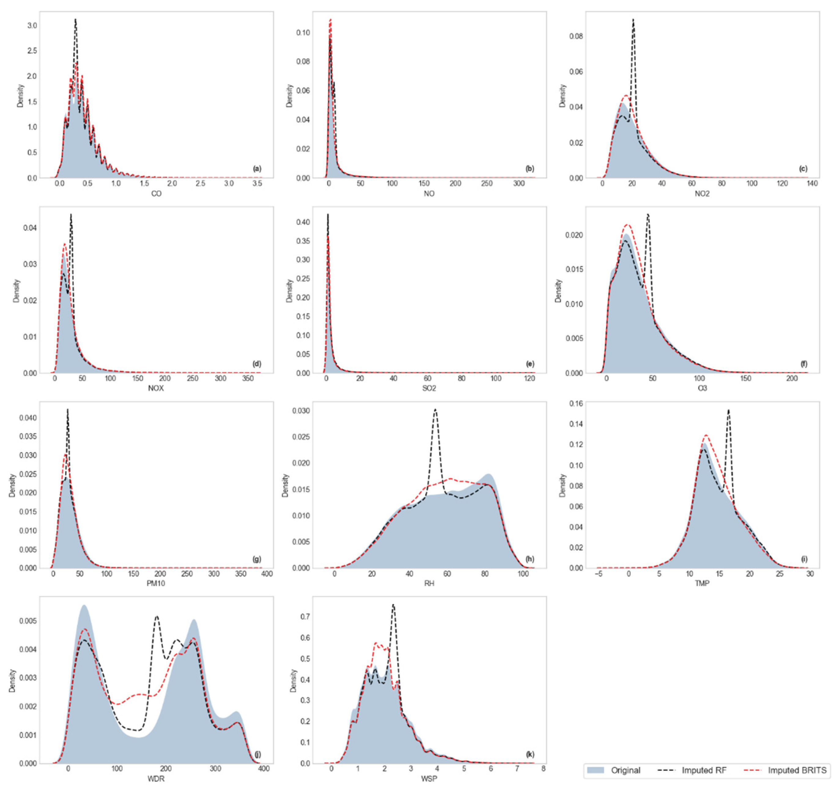
Figure A2.
Kernel Density Estimation (KDE) of original and imputed distributions for FAC station variables.
Figure A2.
Kernel Density Estimation (KDE) of original and imputed distributions for FAC station variables.
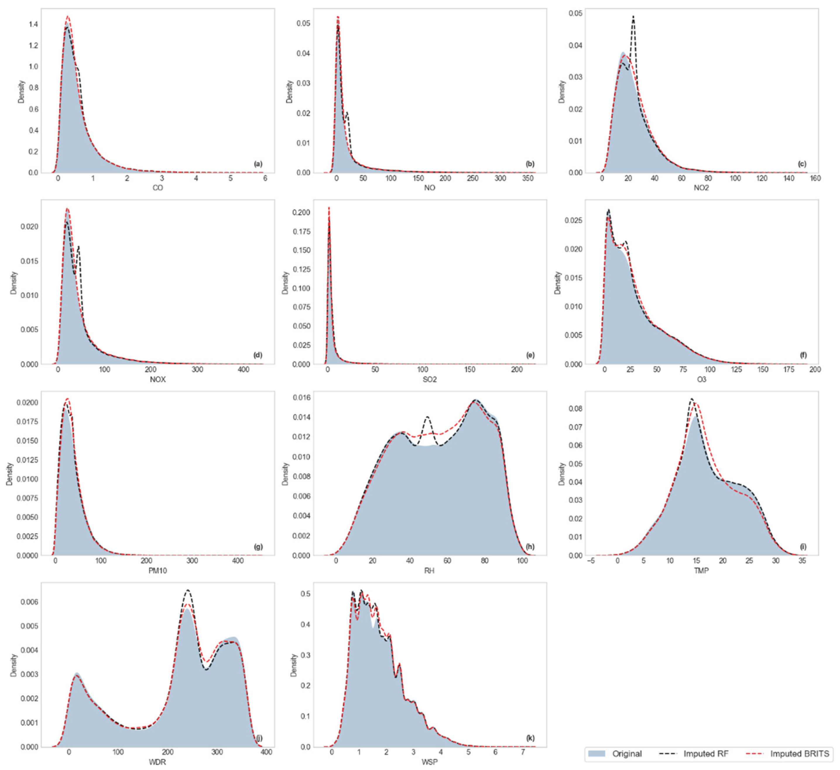
Figure A3.
Kernel Density Estimation (KDE) of original and imputed distributions for MGH station variables.
Figure A3.
Kernel Density Estimation (KDE) of original and imputed distributions for MGH station variables.
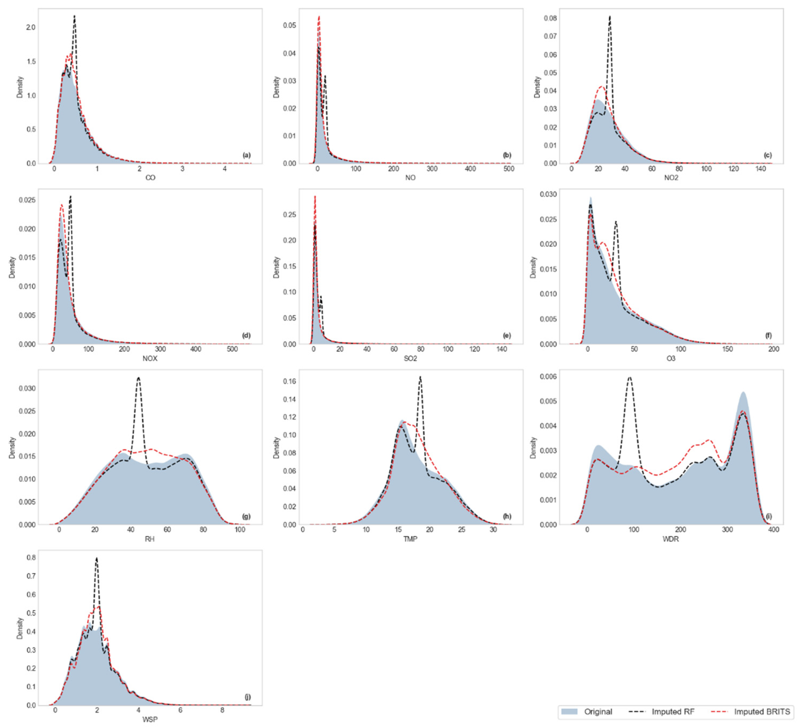
Figure A5.
Kernel Density Estimation (KDE) of original and imputed distributions for NEZ station variables.
Figure A5.
Kernel Density Estimation (KDE) of original and imputed distributions for NEZ station variables.
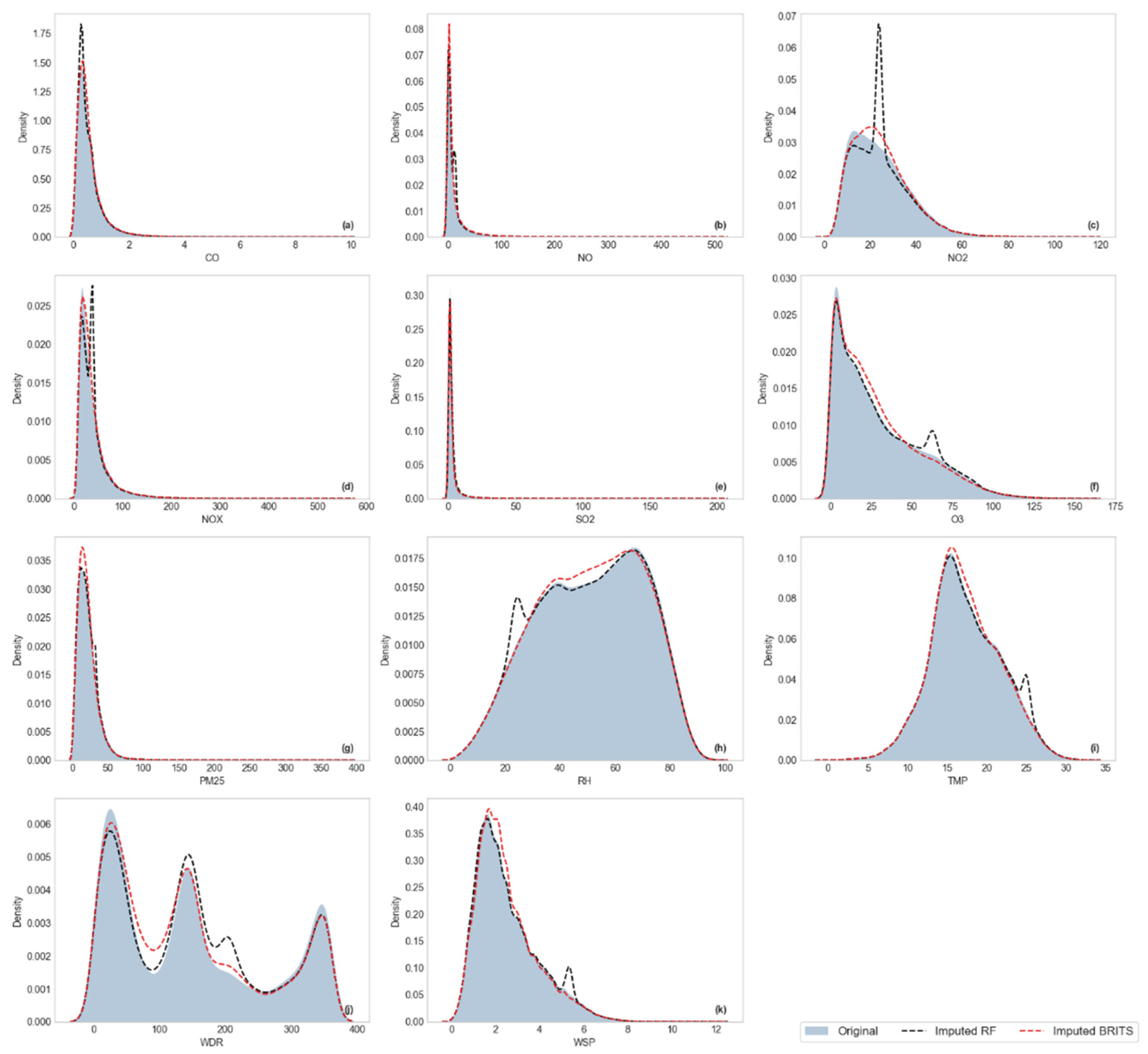
Figure A6.
Kernel Density Estimation (KDE) of original and imputed distributions for PED station variables.
Figure A6.
Kernel Density Estimation (KDE) of original and imputed distributions for PED station variables.
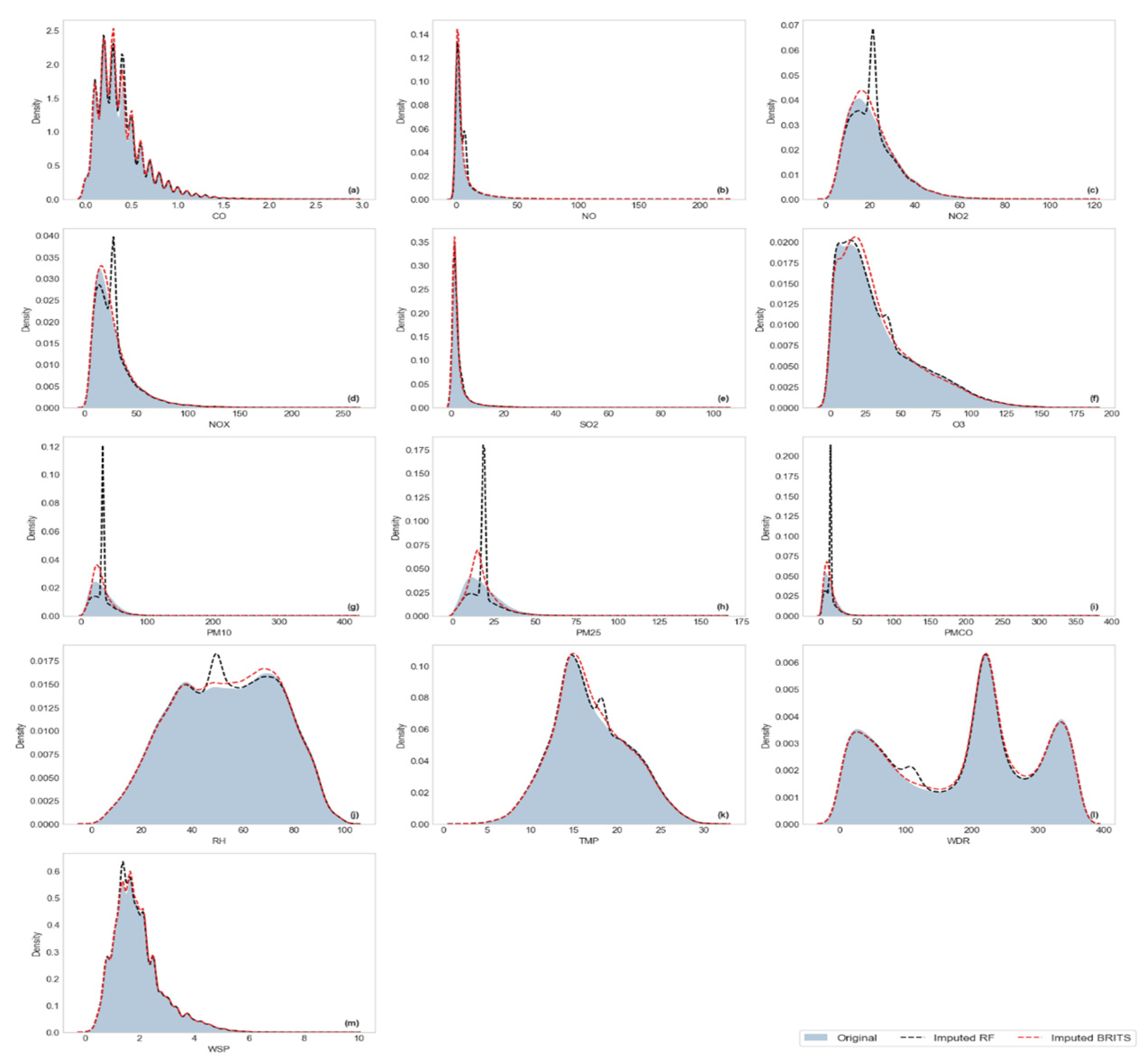
Figure A7.
Kernel Density Estimation (KDE) of original and imputed distributions for SAG station variables.
Figure A7.
Kernel Density Estimation (KDE) of original and imputed distributions for SAG station variables.
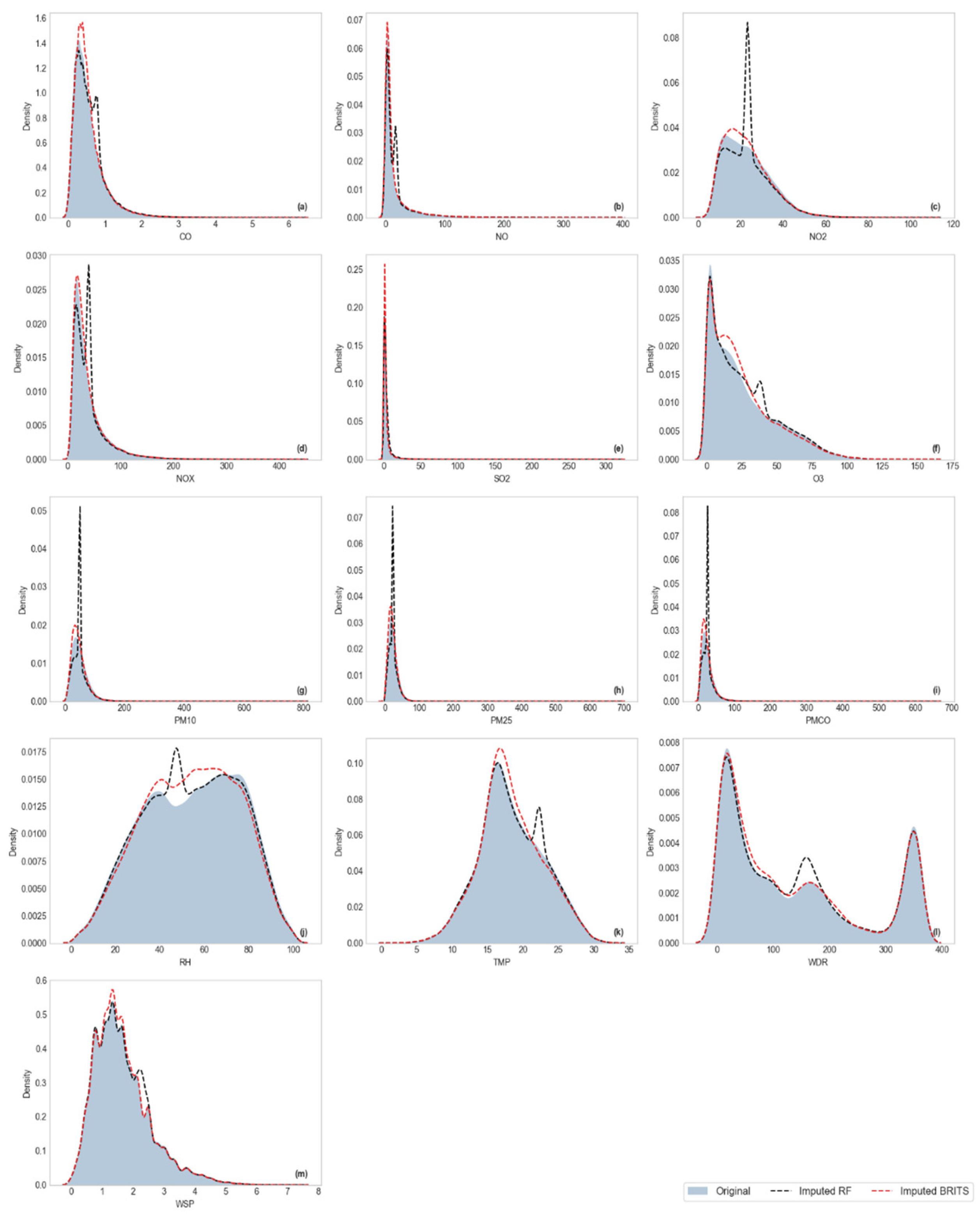
Figure A7.
Kernel Density Estimation (KDE) of original and imputed distributions for TLA station variables.
Figure A7.
Kernel Density Estimation (KDE) of original and imputed distributions for TLA station variables.
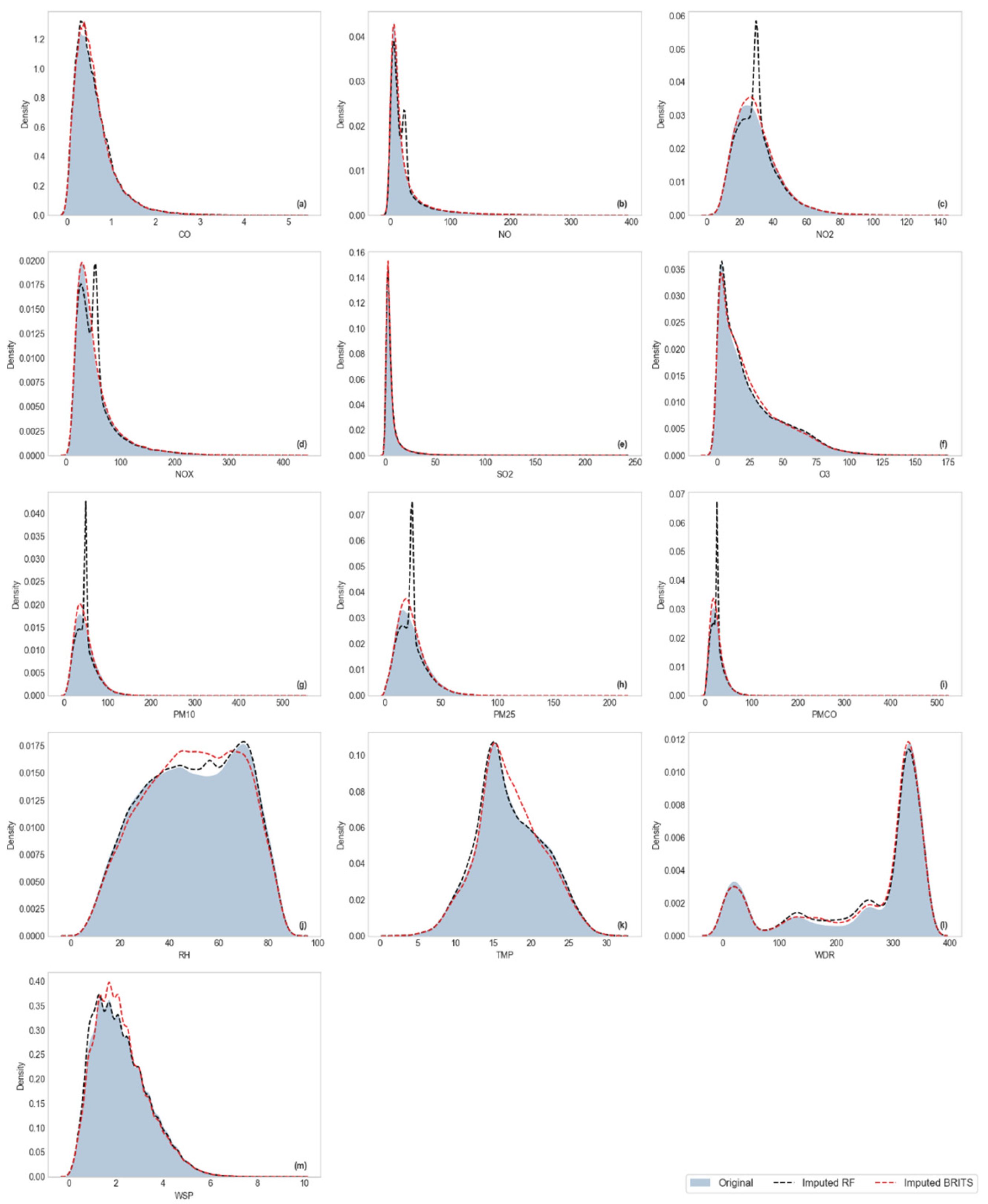
Figure A8.
Kernel Density Estimation (KDE) of original and imputed distributions for UAX station variables.
Figure A8.
Kernel Density Estimation (KDE) of original and imputed distributions for UAX station variables.
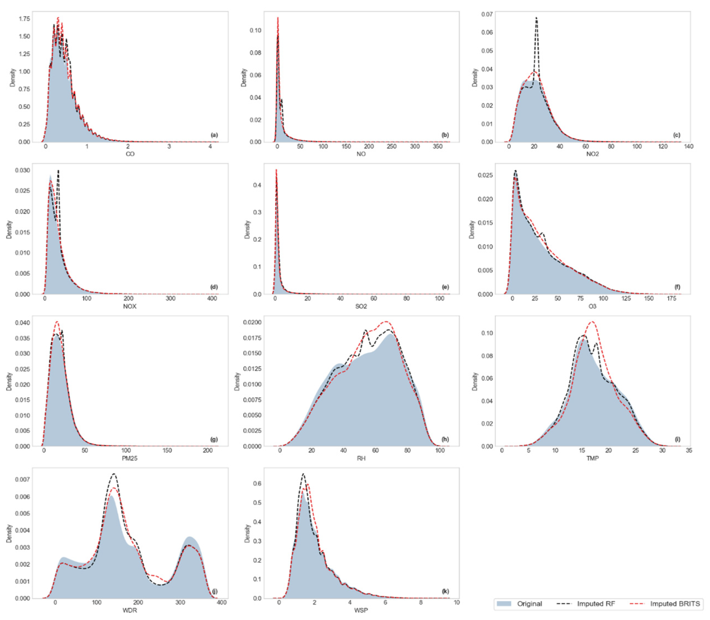
Figure A9.
Kernel Density Estimation (KDE) of original and imputed distributions for VIF station variables.
Figure A9.
Kernel Density Estimation (KDE) of original and imputed distributions for VIF station variables.
References
- World Health Organization (WHO). Ambient (Outdoor) Air Pollution. Available online: https://www.who.int/news-room/fact-sheets/detail/ambient- (accessed on day month year).
- State of Global Air (SoGA). State of Global Air Report 2024. Available online: https://www.stateofglobalair.org/hap (accessed on 19 July 2025).
- World Health Organization (WHO). Air Pollution. Available online: https://www.who.int/health-topics/air-pollution#tab=tab_1 (accessed on 19 July 2025).
- Kim, T.; Kim, J.; Yang, W.; Lee, H.; Choo, J. Missing Value Imputation of Time-Series Air-Quality Data via Deep Neural Networks. Int. J. Environ. Res. Public Health 2021, 18, 12213. [Google Scholar] [CrossRef] [PubMed]
- He, M.Z.; Yitshak-Sade, M.; Just, A.C.; Gutiérrez-Avila, I.; Dorman, M.; de Hoogh, K.; Kloog, I. Predicting Fine-Scale Daily NO₂ over Mexico City Using an Ensemble Modeling Approach. Atmos. Pollut. Res. 2023, 14, 101763. [Google Scholar] [CrossRef] [PubMed]
- Gobierno de México. Programa de Gestión para Mejorar la Calidad del Aire (PROAIRE). Available online: https://www.gob.mx/semarnat/acciones-y-programas/programas-de-gestion-para-mejorar-la-calidad-del-aire (accessed on 19 July 2025).
- Gobierno de la Ciudad de México. Mexico City Atmospheric Monitoring System (SIMAT). Available online: http://www.aire.cdmx.gob.mx/default.php (accessed on 19 July 2025).
- Zhang, X.; Zhou, P. A Transferred Spatio-Temporal Deep Model Based on Multi-LSTM Auto-Encoder for Air Pollution Time Series Missing Value Imputation. Future Gener. Comput. Syst. 2024, 156, 325–338. [Google Scholar] [CrossRef]
- Wang, Y.; Liu, K.; He, Y.; Fu, Q.; Luo, W.; Li, W.; Xiao, S. Research on Missing Value Imputation to Improve the Validity of Air Quality Data Evaluation on the Qinghai-Tibetan Plateau. Atmosphere 2023, 14, 1821. [Google Scholar] [CrossRef]
- Hua, V.; Nguyen, T.; Dao, M.S.; Nguyen, H.D.; Nguyen, B.T. The Impact of Data Imputation on Air Quality Prediction Problem. PLoS ONE 2024, 19, e0306303. [Google Scholar] [CrossRef] [PubMed]
- Alkabbani, H.; Ramadan, A.; Zhu, Q.; Elkamel, A. An Improved Air Quality Index Machine Learning-Based Forecasting with Multivariate Data Imputation Approach. Atmosphere 2022, 13, 1144. [Google Scholar] [CrossRef]
- Camastra, F.; Capone, V.; Ciaramella, A.; Riccio, A.; Staiano, A. Prediction of Environmental Missing Data Time Series by Support Vector Machine Regression and Correlation Dimension Estimation. Environ. Model. Softw. 2022, 150, 105343. [Google Scholar] [CrossRef]
- Che, Z.; Purushotham, S.; Cho, K.; Sontag, D.; Liu, Y. Recurrent Neural Networks for Multivariate Time Series with Missing Values. Sci. Rep. 2018, 8, 6085. [Google Scholar] [CrossRef] [PubMed]
- Cao, W.; Wang, D.; Li, J.; Zhou, H.; Li, L.; Li, Y. BRITS: Bidirectional Recurrent Imputation for Time Series. Adv. Neural Inf. Process. Syst. 2018, 31, 6775–6785. [Google Scholar]
- Yoon, J.; Jordon, J.; Schaar, M. GAIN: Missing Data Imputation Using Generative Adversarial Nets. In Proceedings of the 35th International Conference on Machine Learning, Stockholm, Sweden, 10–15 July 2018; pp. 5689–5698. [Google Scholar]
- Shahbazian, R.; Greco, S. Generative Adversarial Networks Assist Missing Data Imputation: A Comprehensive Survey and Evaluation. IEEE Access 2023, 11, 88908–88928. [Google Scholar] [CrossRef]
- Cini, A.; Marisca, I.; Alippi, C. Filling the Gaps: Multivariate Time Series Imputation by Graph Neural Networks. arXiv 2021, arXiv:2108.00298. [Google Scholar] [CrossRef]
- Du, W.; Côté, D.; Liu, Y. SAITS: Self-Attention-Based Imputation for Time Series. Expert Syst. Appl. 2023, 219, 119619. [Google Scholar] [CrossRef]
- Colorado Cifuentes, G.U.; Flores Tlacuahuac, A. A Short-Term Deep Learning Model for Urban Pollution Forecasting with Incomplete Data. Can. J. Chem. Eng. 2021, 99, S417–S431. [Google Scholar] [CrossRef]
- Alahamade, M.; Lake, A. Handling Missing Data in Air Quality Time Series: Evaluation of Statistical and Machine Learning Approaches. Atmosphere 2021, 12, 1130. [Google Scholar] [CrossRef]
- World Population Review. Mexico City Population. Available online: https://worldpopulationreview.com/cities/mexico/mexico-city (accessed on 19 July 2025).
- Santamaría-Bonfil, G.; Santoyo, E.; Díaz-González, L.; Arroyo-Figueroa, G. Equivalent Imputation Methodology for Handling Missing Data in Compositional Geochemical Databases of Geothermal Fluids. Geothermics 2022, 104, 102440. [Google Scholar] [CrossRef]
- Farjallah, R.; Selim, B.; Jaumard, B.; Ali, S.; Kaddoum, G. Evaluation of Missing Data Imputation for Time Series without Ground Truth. arXiv, 2503. [Google Scholar] [CrossRef]
Figure 1.
Heatmap of missing data percentages for each variable across monitoring stations. Variables with more than 30% missing data are highlighted in red. Monitoring stations marked with * have less than 30% missing data in all variables (excluding PMCO, PM2.5, and PM10).
Figure 1.
Heatmap of missing data percentages for each variable across monitoring stations. Variables with more than 30% missing data are highlighted in red. Monitoring stations marked with * have less than 30% missing data in all variables (excluding PMCO, PM2.5, and PM10).
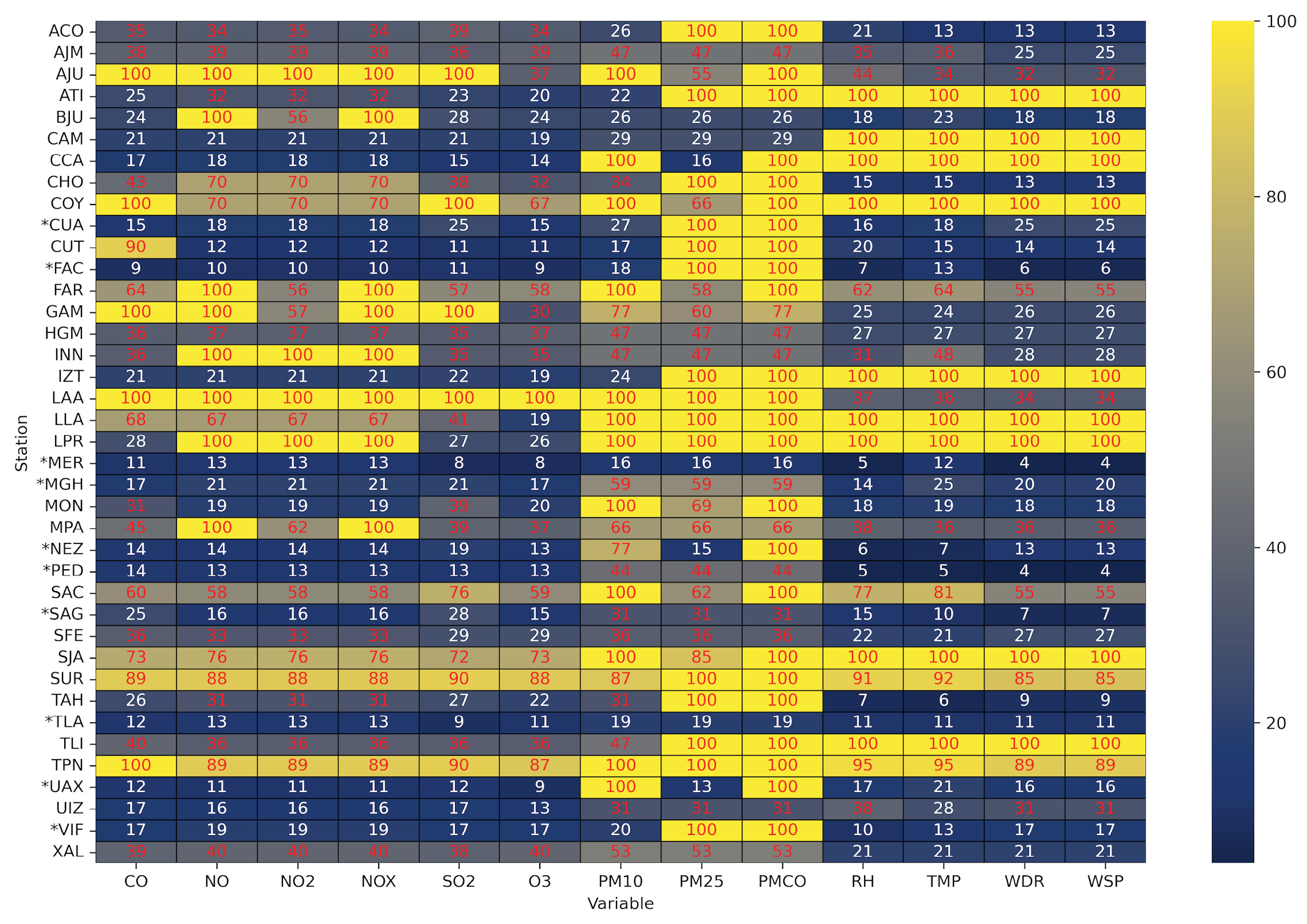
Figure 2.
Map of the Mexico City Atmospheric Monitoring Network (Red Automática de Monitoreo Atmosférico [RAMA]). The stations selected for imputation are marked in blue, because they meet the criterion of having less than 30% missing data in all variables (excluding PM₁₀, PM₂.₅, and PMCO).
Figure 2.
Map of the Mexico City Atmospheric Monitoring Network (Red Automática de Monitoreo Atmosférico [RAMA]). The stations selected for imputation are marked in blue, because they meet the criterion of having less than 30% missing data in all variables (excluding PM₁₀, PM₂.₅, and PMCO).
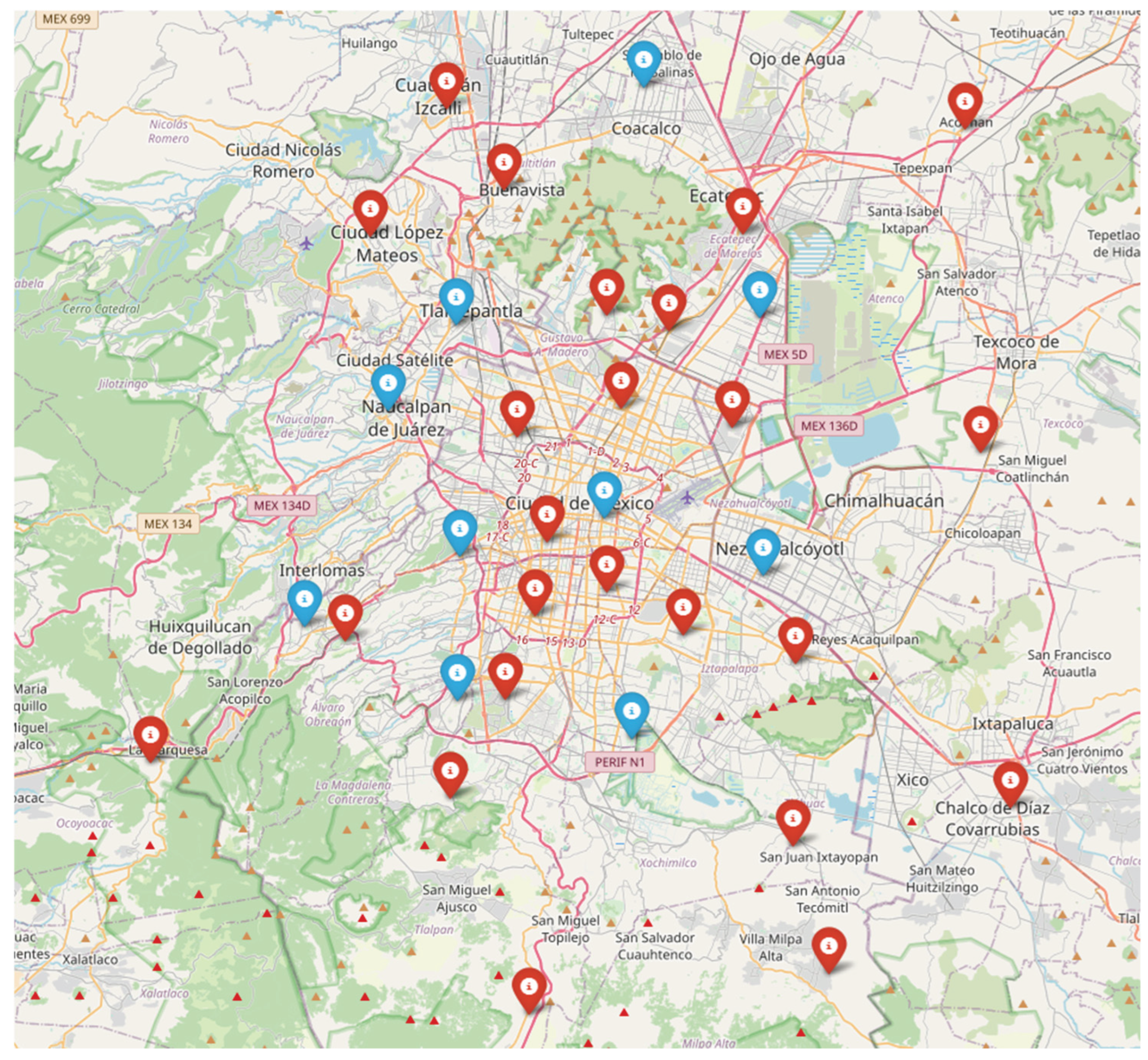
Figure 3.
Percentage of missing values for each variable across the selected stations.
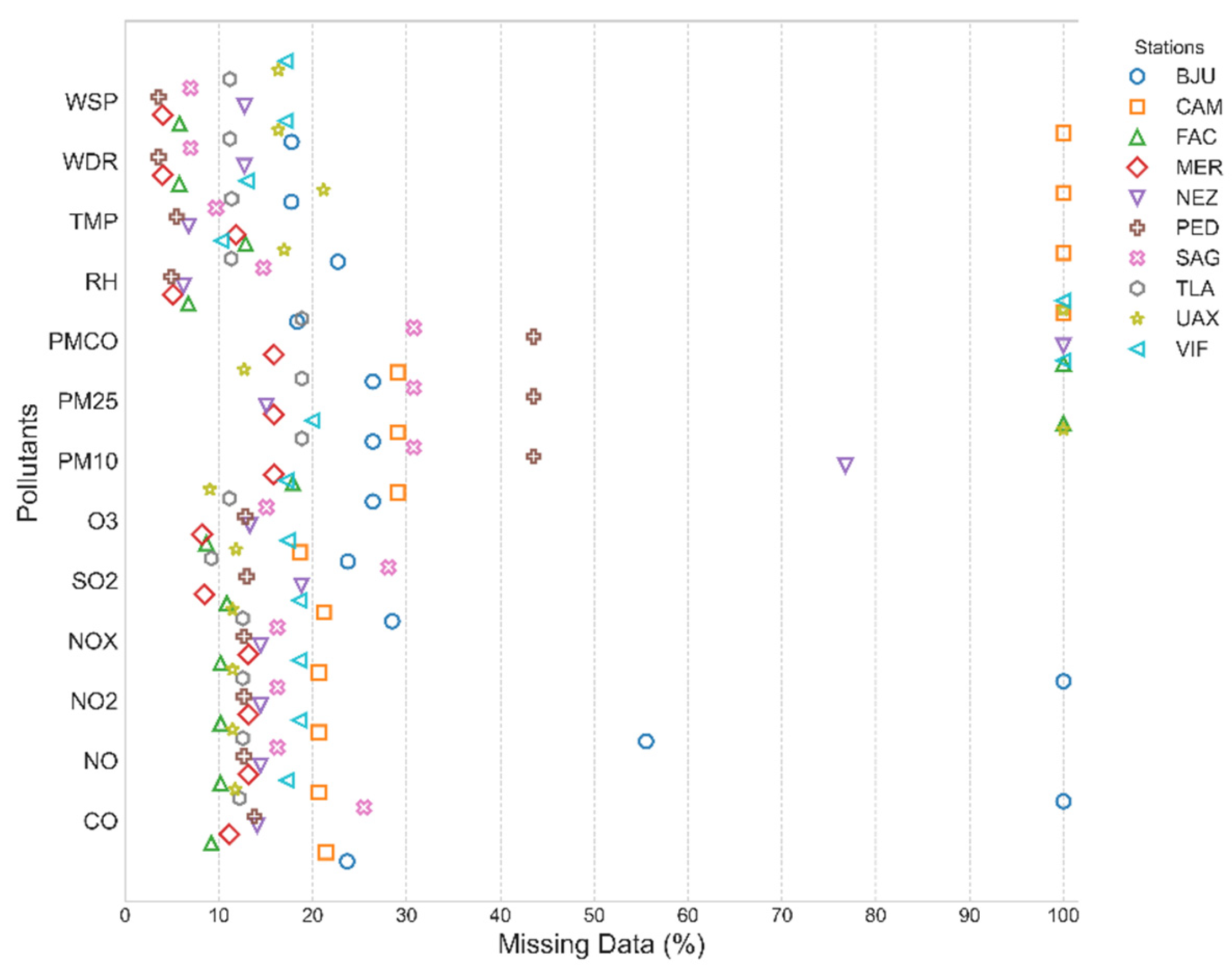
Figure 4.
Temporal structure of missing data for the selected monitoring stations.
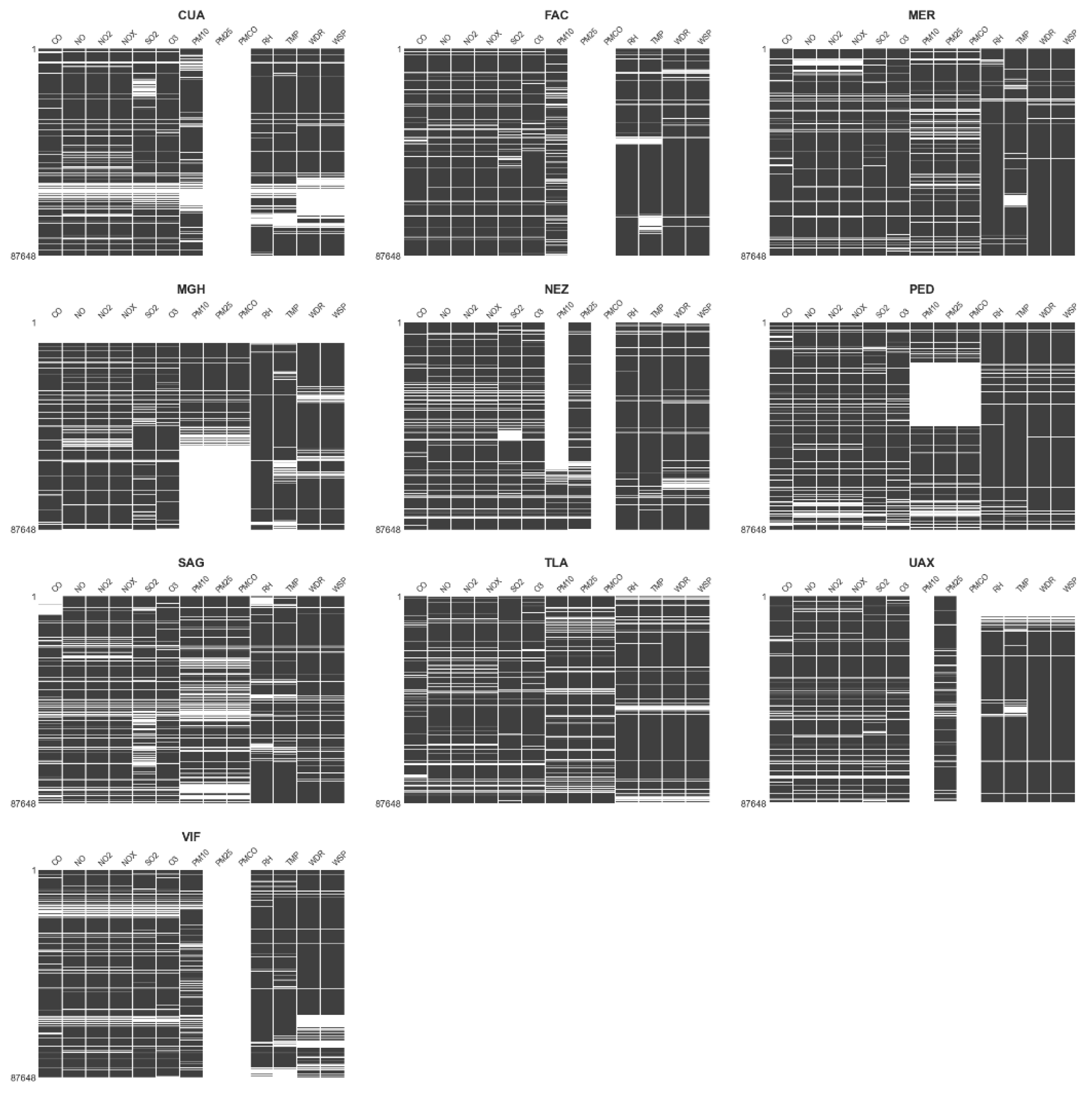
Figure 5.
Boxplots of Mean Absolute Error (MAE) for Random Forest (RF) and BRITS across all variables and stations. These values were computed using 20% of observed values randomly masked from the validation set. Each subplot corresponds to a single variable, maintaining its original measurement scale.
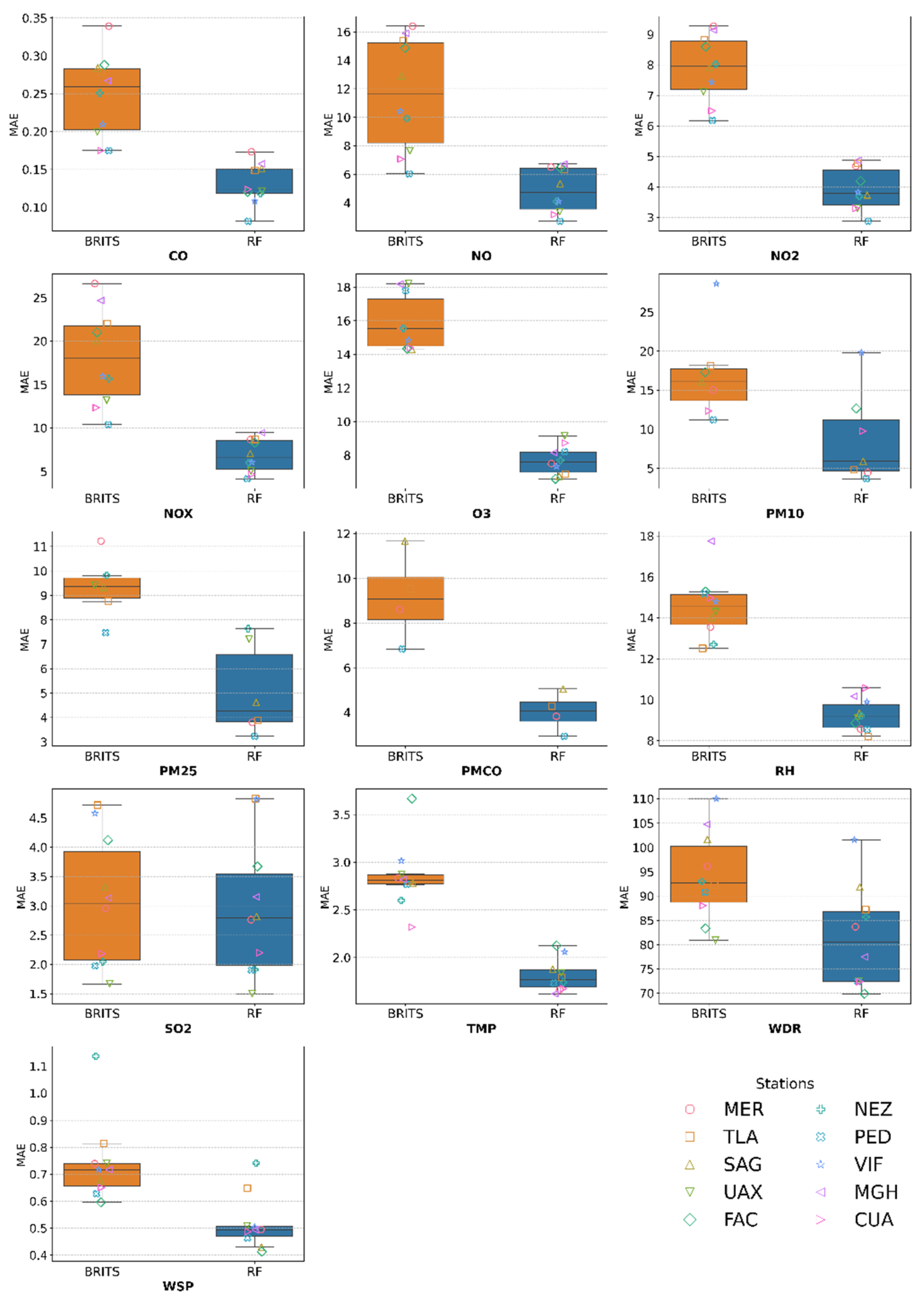
Figure 6.
Boxplots of Root Mean Squared Error (RMSE) for RF and BRITS across all variables and stations; that were computed on masked sets. Each subplot corresponds to a different variable with its original scale.
Figure 6.
Boxplots of Root Mean Squared Error (RMSE) for RF and BRITS across all variables and stations; that were computed on masked sets. Each subplot corresponds to a different variable with its original scale.
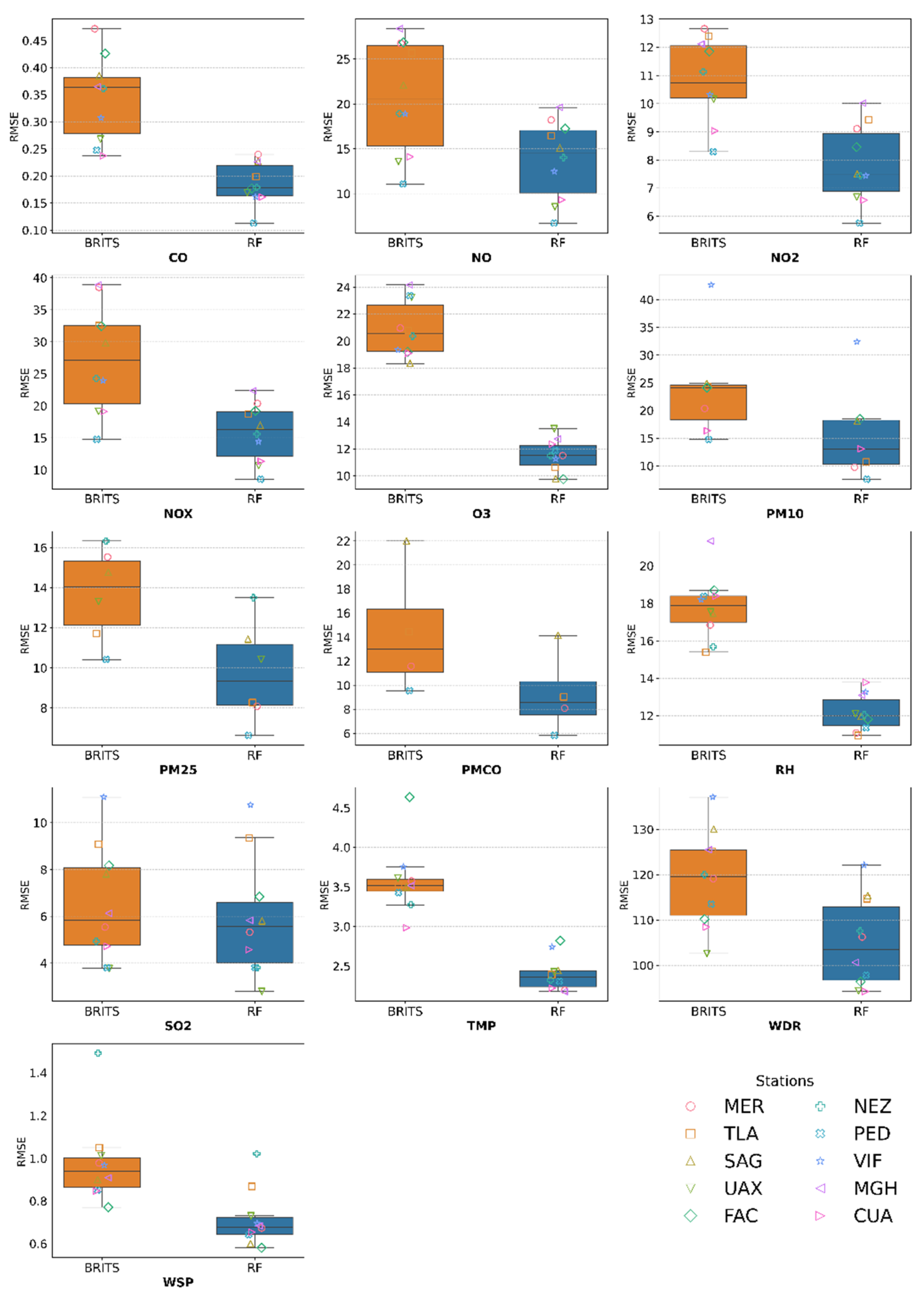
Figure 7.
Boxplots of Wasserstein Distance for RF and BRITS across all variables and stations. These values were calculated on complete distribution of each variable: original database versus imputed database. Each subplot corresponds to a specific variable.
Figure 7.
Boxplots of Wasserstein Distance for RF and BRITS across all variables and stations. These values were calculated on complete distribution of each variable: original database versus imputed database. Each subplot corresponds to a specific variable.
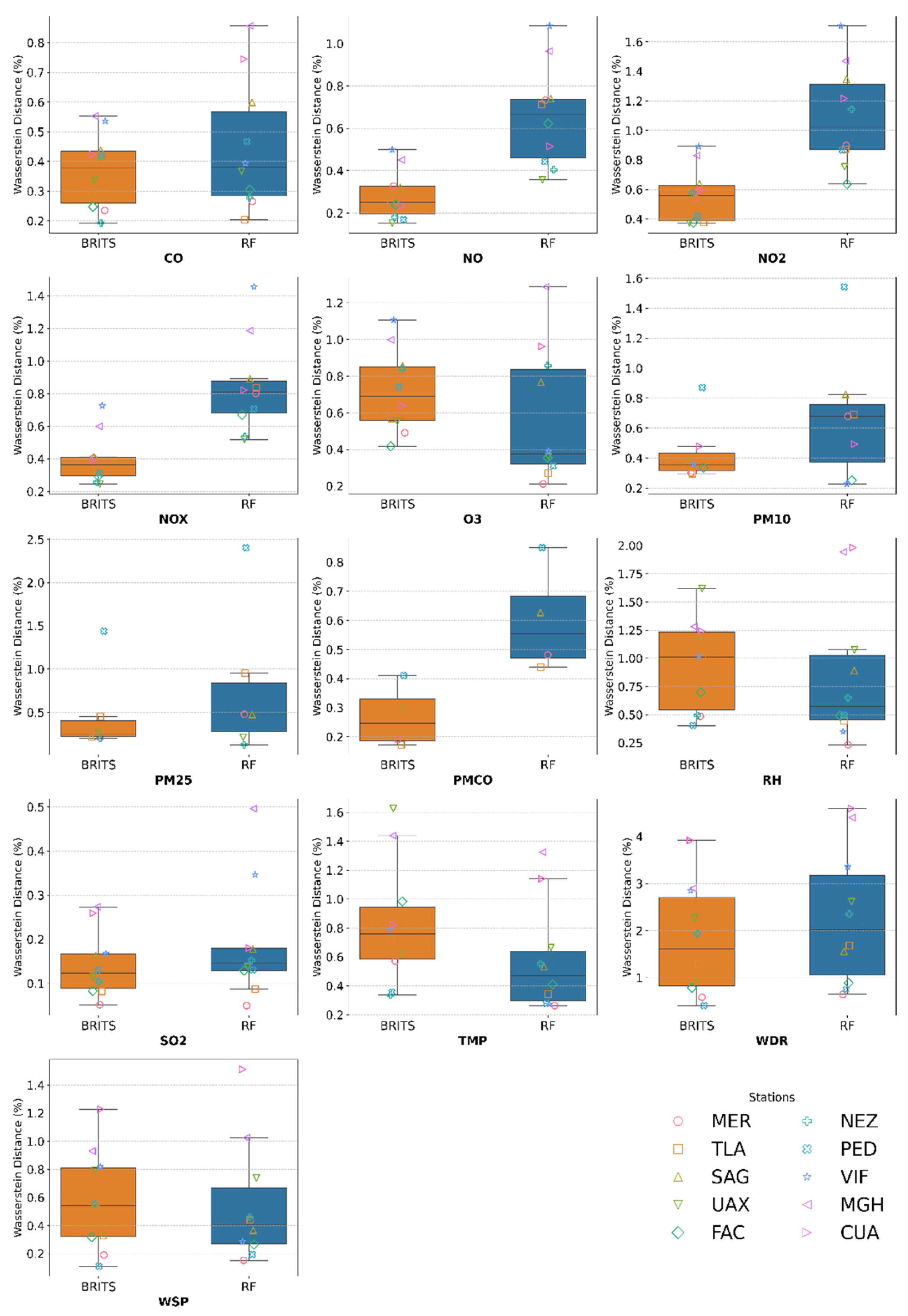
Figure 8.
Comparison original and imputed means for RF and BRITS with TOST equivalence intervals across stations. TOST was applied to the complete distribution of each variable, comparing the original dataset with the imputed dataset.
Figure 8.
Comparison original and imputed means for RF and BRITS with TOST equivalence intervals across stations. TOST was applied to the complete distribution of each variable, comparing the original dataset with the imputed dataset.
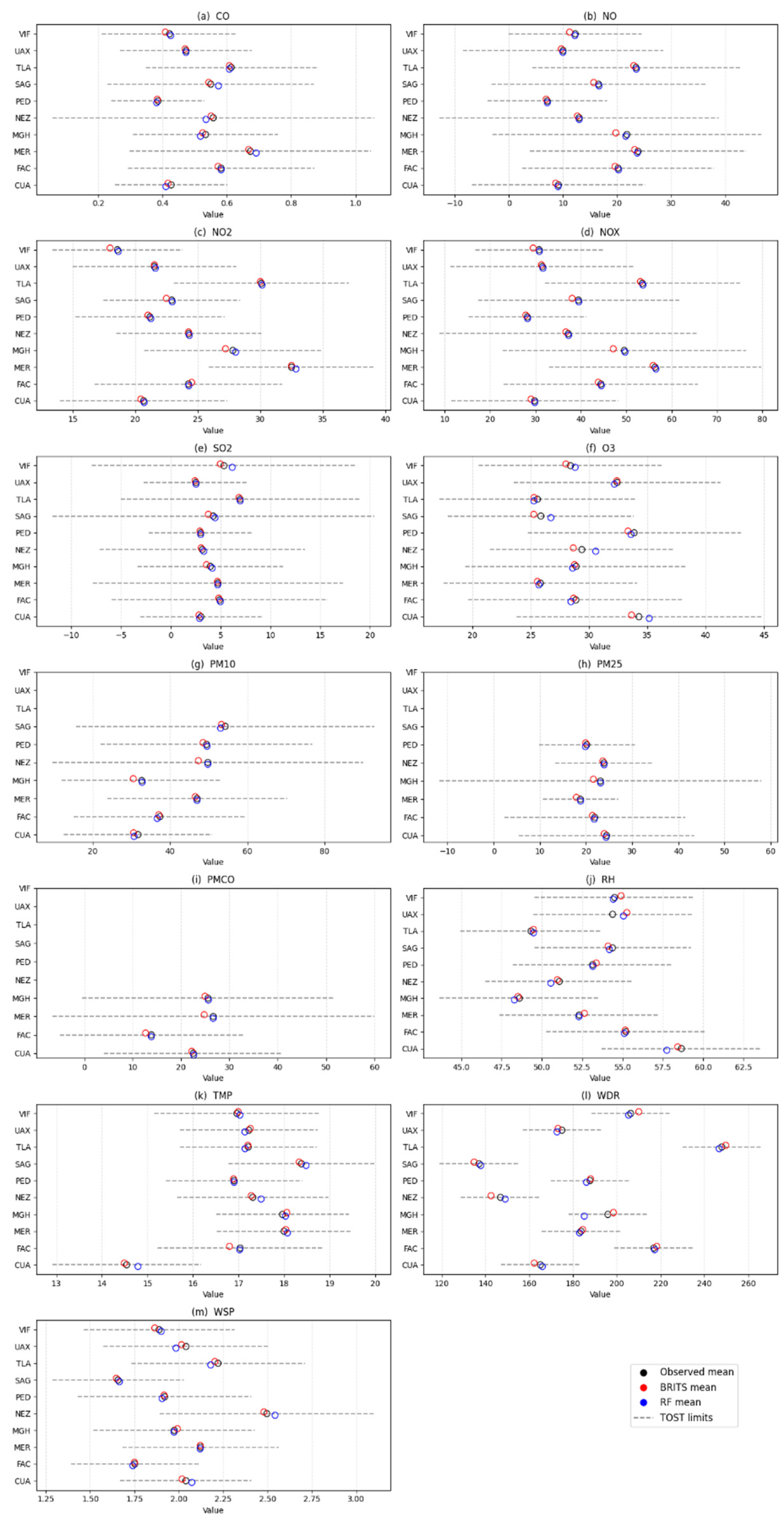
Figure 9.
Kernel Density Estimation (KDE) of original and imputed distributions for MER station variables.
Figure 9.
Kernel Density Estimation (KDE) of original and imputed distributions for MER station variables.
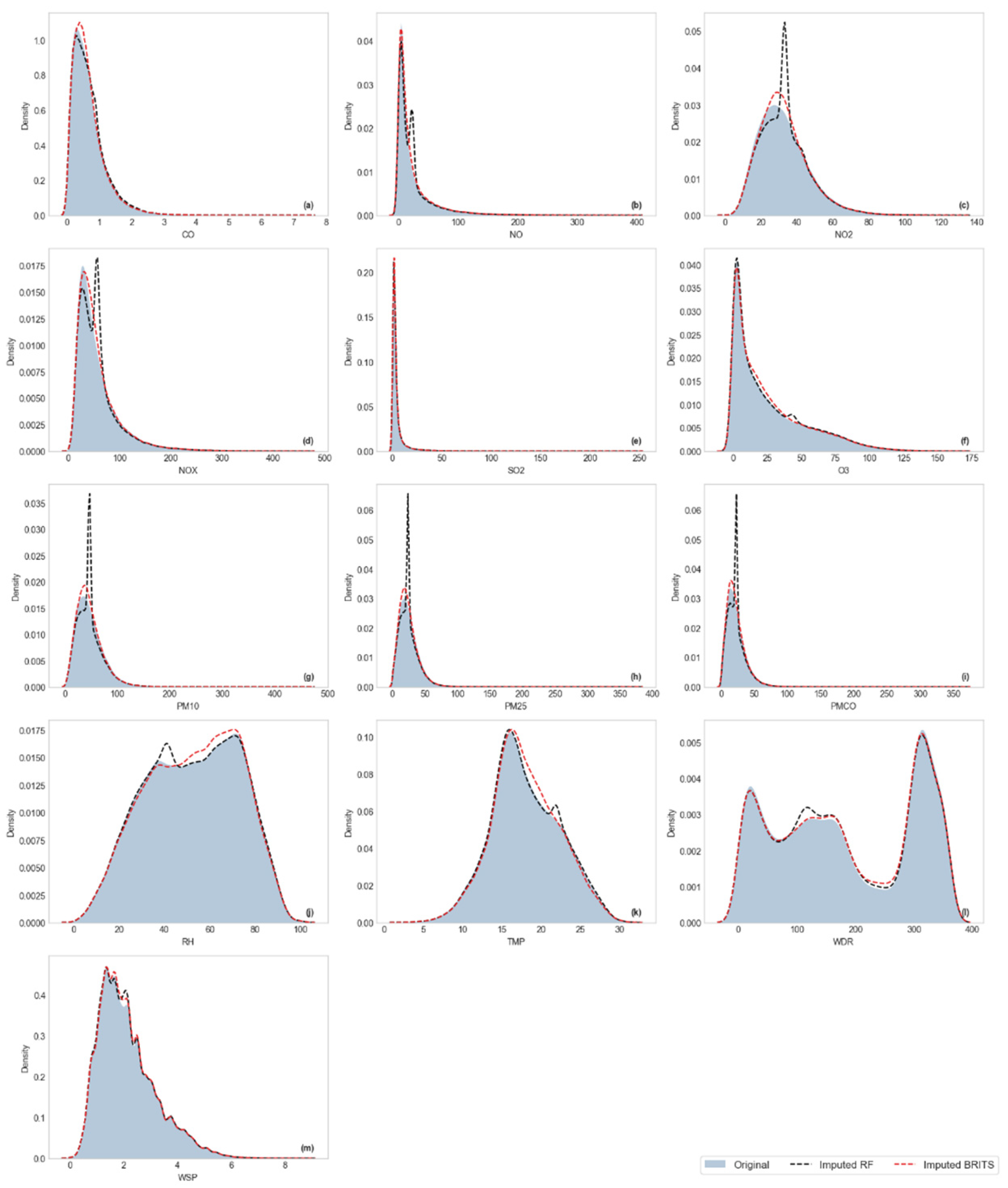
Figure 10.
Complete time series from 2014 to 2023 for the MER station, showing observed values (blue) and imputed values using BRITS (yellow).
Figure 10.
Complete time series from 2014 to 2023 for the MER station, showing observed values (blue) and imputed values using BRITS (yellow).
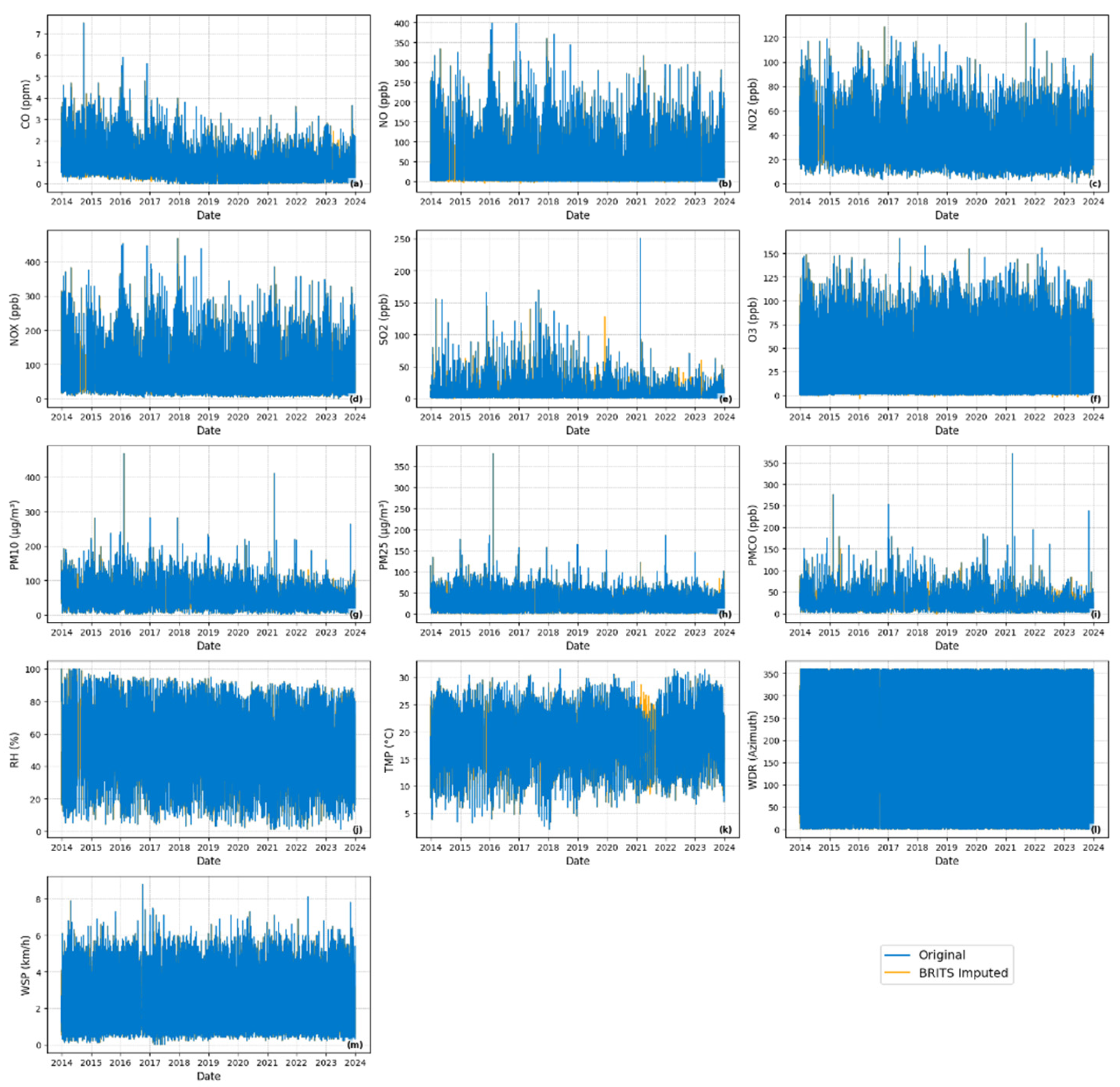
Figure 11.
Complete time series from 2014 to 2023 for the MER station, showing observed values (blue) and imputed values using Random Forest (yellow).
Figure 11.
Complete time series from 2014 to 2023 for the MER station, showing observed values (blue) and imputed values using Random Forest (yellow).
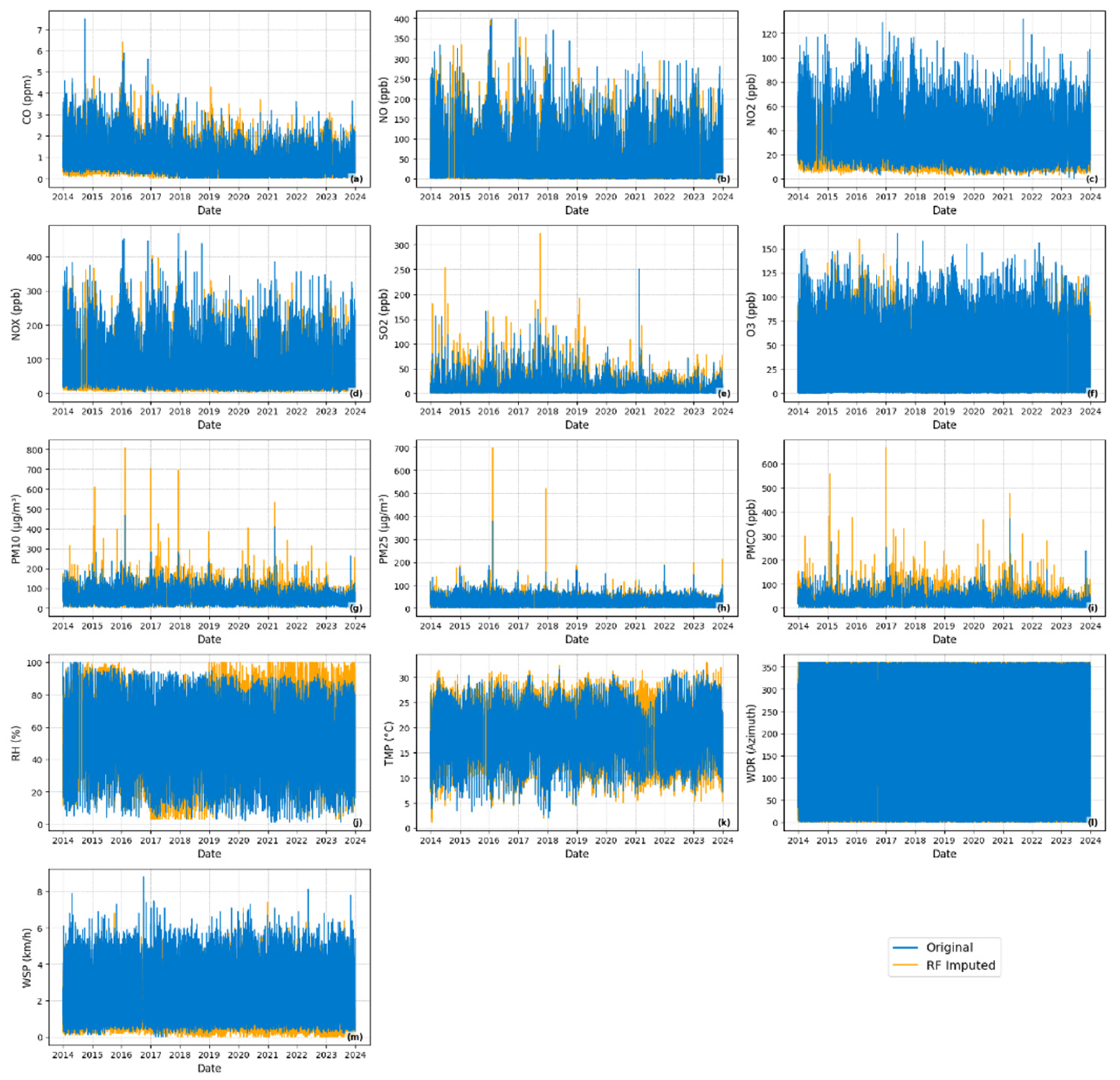
Table 1.
Summary of recent studies on air quality data imputation and prediction.
| Reference | Datasets and Missing Rate | Input Variables and Missing Rate | Techniques | Target | Key Findings |
|---|---|---|---|---|---|
| Kim et al. (2021) [4] | Minute-level air quality data (2020–2021) from South Korea: Guro-gu (24 stations) and Dangjin-si (42 stations). | PM₂.₅ and PM₁₀ concentrations. Missing Rate (Real / Artificial): 7.91–16.1% / 20%. |
A novel N-BEATS deep learning model with interpretable blocks (trend, seasonality, residual) was compared with baseline methods (mean, spatial average, MICE). | Imputation of missing PM₂.₅ and PM₁₀ values. | N-BEATS model outperforms traditional methods and allows interpretability via component decomposition but struggles with long-term seasonal patterns due to fixed-period Fourier terms. |
| Alahamade & Lake (2021) [20] | Hourly pollutant data (PM₁₀, PM₂.₅, O₃, NO₂) of the Automatic Urban and Rural Network (AURN) from UK (2015-2017), covering 167 station types (urban, suburban, rural, roadside, industrial). | Concentrations of PM₁₀, PM₂.₅, O₃ and NO₂. Missing Rate (Real / Artificial): Not quantified (some pollutants entirely missing at certain stations) / Not applied |
Evaluated models: (1) Clustering based on multivariate time series similarity (CA, CA+ENV, CA+REG); (2) Spatial methods using the 1 or 2 nearest stations (1NN, 2NN); (3) Ensemble method: median of all five approaches. | Imputation of missing PM₁₀, PM₂.₅, O₃ and NO₂ using temporal and spatial similarity. | The ensemble method performed best for O₃, PM₁₀, and PM₂.₅, CA+ENV for NO₂. Performance depended on the pollutant and station type. MVTS clustering allowed full imputation; extremes were slightly under- or overestimated. |
| Wang et al. (2023) [9] | Hourly air quality data (2019–2022) from 16 stations in Qinghai Province and Haidong City, China. | Multivariate time series of six pollutants (PM2.5, PM10, O3, NO2, SO2, and CO). Missing Rate (Real / Artificial): 5–22% / 30%. | BRITS-ALSTM (BRITS encoder + LSTM with attention) was compared to Mean, KNN, MICE, MissForest, M-RNN, BRITS, and BRITS-LSTM. | Imputation of missing pollutants (PM2.5, PM10, O3, NO2, SO2, and CO) data with high and irregular missing rates. | BRITS-ALSTM outperformed baselines for all pollutants and missing patterns. |
| He et al. (2023) [5] | Air quality and meteorological data from Mexico City (2005–2019; 42 stations), combined with satellite data from OMI, TROPOMI, and reanalysis data from CAMS. #stations? |
Daily NO₂ concentrations, wind speed/direction, temperature, cloud coverage, and satellite-based NO₂ columns. Missing Rate (Real / Artificial): Not quantified / Not simulated. |
Comparative modeling using RF, XGBoost, and GAM. Missing values were imputed using Random Forest. | Predict daily NO₂ surface concentrations in Mexico City. | XGBoost and RF outperformed GAM. The model integrated hybrid sources (ground, satellite, and meteorological) to improve NO₂ prediction. |
| Colorado Cifuentes and Flores Tlacuahua (2020) [19] | Hourly air quality and meteorological data (2012-2017) from 13 monitoring stations in the Monterrey Metropolitan area, Mexico. | Pollutants and meteorological variables over a 24-hour window. Missing Rate (Real / Artificial): <25% / Not simulated. |
A deep neural network (DNN). Missing values were imputed using interpolation for non-seasonal time series. | 24-hour ahead prediction of O₃, PM₂.₅, and PM₁₀. |
The DNN model achieved good predictive accuracy for all target pollutants, and the imputation process preserved model performance. |
| Hua et al. (2024) [10] | Six real-world hourly datasets from Germany, China, Taiwan, and Vietnam. The datasets include ~15,000 to 1.2 million samples. | Pollutant and meteorological variables. Missing Rate (Real / Artificial): 0-42% / 10-80%. |
Mean, Median, KNN, MICE, SAITS, BRITS, MRNN, and Transformer. | Evaluate the impact of different imputation strategies on the performance of air quality forecasting models, aimed at predicting 24-hour concentrations of AQI, PM₂.₅, PM₁₀, CO, SO₂, and O₃. | SAITS achieved the highest accuracy, followed by BRITS. KNN performed well on large datasets with high missing rates. MICE was effective on smaller datasets but was slower. Transformer model performed worse than the top methods. |
| Zhang and Zhou (2024) [8] | PM2.5 time series (2018-2020; 225 stations) from Xi’an, China, with single, block, and long-interval missing patterns. | PM2.5 data from multiple stations, with spatial-temporal dependencies. Missing Rate (Real / Artificial): <1% / [10%, 20%, 30%, 50%] | TMLSTM-AE was compared to KNN, SVD, ST-MVL, LSTM, and DAE | Impute complex missing patterns in single-feature PM2.5 time series using spatial-temporal dependencies. | TMLSTM-AE outperforms traditional and baselines methods, especially on long and block missing data. |
1NN: One Nearest Neighbor; 2NN: Two Nearest Neighbors; BRITS: Bidirectional Recurrent Imputation for Time Series; BRITS-ALSTM: BRITS encoder + LSTM decoder with Attention mechanism; BRITS-LSTM: BRITS encoder + LSTM decoder (Seq2Seq); CA: Cluster Average; CA+ENV: Cluster Average within the same station type (Environmental category); CA+REG: Cluster Average within the same region; CAMS: Global atmospheric reanalysis data; DAE: Deep autoencoder; DNN: Deep neural network; GAM: Generalized Additive Model; KNN: k-nearest neighbors; LSTM: Long short-term memory; MICE: Multivariate Imputation by Chained Equations; MRNN: Multi-directional Recurrent Neural Network; MVTS: Multivariate Time Series; N-BEATS: Neural basis expansion analysis for interpretable time series forecasting; OMI: Satellite sensor for atmospheric pollutants; RAMA: Air quality monitoring network in Mexico City; RF: Random Forest; SAITS: Self-Attention-based Imputation for Time Series; ST-MVL: Spatio-temporal multi-view learning; SVD: Singular value decomposition; TMLSTM-AE: Deep model combining LSTM, autoencoder, and transfer learning; TROPOMI: Satellite instrument for tropospheric pollution; XGBoost: Extreme Gradient Boosting.
Table 2.
Random Forest and BRIST hyperparameter optimization details used in this study.
| Hyperparameter | default value | values evaluated |
|---|---|---|
| (a) RandomForest | ||
| n_estimators | 100 | [10, 20, 50, 80] |
| max_depth | None | [10, 20, None] |
| max_iter* | 10 | [5, 10, 15, 20] |
| min_samples_split | 2 | [2, 5, 10, 15] |
| min_samples_leaf | 1 | [1, 2, 4, 6] |
| (a) BRITS | ||
| RNN units | 64 | [64, 128, 256, 512] |
| subsequence length | 24 | [16, 32, 64, 128, 168] |
| learning rate | 0.001 | [0.001, 0.005, 0.009] |
| batch size | 64 | [16, 32, 64, 128, 168] |
| use regularization | False | [False, True] |
| dropout rate | 0 | [0.10, 0.2, 0.30] |
Table 3.
Random Forest hyperparameter optimization details for the 10 imputed station datasets used in this study.
Table 3.
Random Forest hyperparameter optimization details for the 10 imputed station datasets used in this study.
| Hyperparameter | default value | values evaluated | Best parameters for each station | |||||||||
|---|---|---|---|---|---|---|---|---|---|---|---|---|
| PED | MER | SAG | TLA | FAC | NEZ | UAX | CUA | VIF | MGH | |||
| n_estimators | 100 | [10, 20, 50, 80] | 50 | 20 | 50 | 20 | 50 | 20 | 20 | 10 | 20 | 10 |
| max_depth | None | [10, 20, None] | 20 | 20 | 20 | None | None | 20 | 10 | 10 | 20 | 10 |
| max_iter* | 10 | [5, 10, 15, 20] | 10 | 15 | 15 | 15 | 5 | 10 | 20 | 15 | 15 | 10 |
| min_samples_split | 2 | [2, 5, 10, 15] | 5 | 10 | 2 | 2 | 2 | 10 | 5 | 15 | 15 | 10 |
| min_samples_leaf | 1 | [1, 2, 4, 6] | 1 | 4 | 4 | 4 | 1 | 6 | 4 | 4 | 6 | 4 |
Table 4.
BRITS hyperparameter optimization details for the 10 imputed station datasets used in this study.
Table 4.
BRITS hyperparameter optimization details for the 10 imputed station datasets used in this study.
| Hyperparameter | default value | values evaluated | Best parameters for each station | |||||||||
|---|---|---|---|---|---|---|---|---|---|---|---|---|
| PED | MER | SAG | TLA | FAC | NEZ | UAX | CUA | VIF | MGH | |||
| RNN units | 64 | [64, 128, 256, 512] | 512 | 512 | 512 | 512 | 256 | 512 | 512 | 256 | 256 | 512 |
| subsequence length | 24 | [16, 32, 64, 128, 168] | 32 | 64 | 64 | 32 | 128 | 64 | 64 | 32 | 64 | 168 |
| learning rate | 0.001 | [0.001, 0.005, 0.009] | 0.005 | 0.005 | 0.005 | 0.005 | 0.005 | 0.005 | 0.005 | 0.005 | 0.005 | 0.009 |
| batch size | 64 | [16, 32, 64, 128, 168] | 32 | 32 | 32 | 32 | 32 | 32 | 32 | 32 | 32 | 128 |
| use regularization | False | [False, True] | True | False | True | False | False | True | False | False | True | False |
| dropout rate | 0 | [0.10, 0.2, 0.30] | 0.2 | 0.2 | 0.2 | 0.2 | 0.2 | 0.2 | 0.2 | 0.3 | 0.1 | 0.1 |
Disclaimer/Publisher’s Note: The statements, opinions and data contained in all publications are solely those of the individual author(s) and contributor(s) and not of MDPI and/or the editor(s). MDPI and/or the editor(s) disclaim responsibility for any injury to people or property resulting from any ideas, methods, instructions or products referred to in the content. |
© 2025 by the authors. Licensee MDPI, Basel, Switzerland. This article is an open access article distributed under the terms and conditions of the Creative Commons Attribution (CC BY) license (http://creativecommons.org/licenses/by/4.0/).
Copyright: This open access article is published under a Creative Commons CC BY 4.0 license, which permit the free download, distribution, and reuse, provided that the author and preprint are cited in any reuse.


