
Submitted:
22 July 2025
Posted:
23 July 2025
You are already at the latest version
Abstract
Most of the existing ultra-deep gas wells in China are characterized by high temperature, high pressure, and high sulfur content. During the development process, they face severe challenges such as unclear mechanisms of acidic gas-induced blowouts and difficulties in wellbore pressure inversion, which pose significant risks to well control operations. To reveal the reasons behind the tendency of acidic gases to trigger blowouts and to clarify the impact of different concentrations of acidic gases on the flow behavior of annular fluids, this study considers the effects of solubility and phase changes on the physical properties of acidic gases. A method replacing critical parameters with pseudo-critical parameters is used to analyze the variation trends of gas density, solubility, and other properties along the well depth. A mathematical model for the annular flow of acidic gas overflow incorporating solubility phase change effects is established. The model is numerically solved using a four-point difference scheme, exploring the essential characteristics of gas flow in the annulus after overflow, and discussing the distribution patterns of physical properties of acidic gases, as well as dynamic parameters such as wellbore pressure and temperature along the well depth. The results indicate that the physical properties of acidic gases change significantly with well depth: the more acidic gas present in the wellbore, the smaller the deviation factor, and the greater the density and viscosity, with parameter changes exceeding 40% near the pseudo-critical point. Compared to pure methane, mixed fluids containing acidic gas experience more than 20% volume expansion near the wellhead, and the flow velocity increases by more than 10%, leading to a higher risk of a sudden pressure drop during well control. This study clarifies the migration patterns of acidic gas overflow in HPHT (high pressure, high temperature)gas wells, providing valuable guidance for optimizing well control design, improving well control emergency plans, and developing well-killing measures.
Keywords:
High pressure
; 10
; 000-meter deep well
; overflow
; annular flow
1. Introduction
The deep to ultra-deep conventional gas resources in major basins of PetroChina amount to 20 trillion cubic meters, indicating enormous exploration potential (Chengzao et al., 2025; Hua et al., 2022; Yuyu et al.). However, with increasing well depths, high-temperature, high-pressure, and high-sulfur conditions pose significant challenges to well control safety (Wang et al., 2024; Xinyu et al., 2024). Table 1 presents statistical data on blowouts caused by acidic gas influx(Qian et al., 2023), revealing that once gas invasion occurs in natural gas containing acidic components, there is a high probability of severe accidents(Feng et al., 2023; Shaomu et al., 2024; Wezehwa et al., 2018). Therefore, it is imperative to investigate the migration mechanisms of acidic gas under high-temperature and high-pressure conditions in ultra-deep wells(Baojiang et al., 2020), ensuring the safe and efficient development of acidic gas reservoirs(Kiran et al., 2019; Krishna et al., 2020).
Today, researchers both domestically and internationally have conducted extensive studies on wellbore gas kicks and gas pollution(Ferroudji et al., 2021; Tang et al., 2022a; Zainith and Mishra, 2021).
In 2012, (Dou et al., 2012) considered the unique physical properties of high-sulfur gases and potential phase changes occurring in the wellbore, developing a mathematical model for wellbore flow and heat transfer during high-sulfur gas overflow. They coupled temperature, pressure, and physical property parameters of high-sulfur gases, and proposed a solution method. The study analyzed the wellbore pressure and gas properties during the ascent of gases with different H₂S contents, concluding that high-sulfur gases can easily lead to well control issues. In 2016, (Wang et al., 2016)developed a temperature field model for CO₂ in the wellbore and fractures to calculate the phase change of fluid and variations in thermophysical parameters during fracturing. The study analyzed the location of CO₂ phase transitions from liquid to supercritical state, finding that the transition point shifted from inside the wellbore toward the fractures. In 2018 (Sun et al., 2018)conducted experimental analysis on the phase changes of acidic gas mixtures during overflow, specifically focusing on the behavior of CO₂ and CH₄ mixtures due to the toxicity of H₂S. The results showed that the physical properties of acidic gas mixtures in the supercritical phase change abruptly near the critical point, leading to significant volume expansion in the wellbore and an increased blowout risk. In 2018, (Xinming et al., 2018) studied the pressure drop and friction factor changes during supercritical CO₂ flow in the wellbore through experiments. They noted that both friction factor and pressure drop increased with higher flow rates and pressures. In 2019, (Zaidin et al., 2019)performed extensive experiments using detailed data on gas and brine compositions in the Sarawak Basin, Malaysia. He estimated the initial CO₂ solubility in brine reservoirs at 423.15 K and 36.0 MPa in the Sarawak Basin. In 2019, (Yuanyuan, 2019)conducted a quantitative analysis of the dissolution process of H₂S in NaCl solution, using normalized Raman peak intensities (peak area ratios and peak height ratios) to quantify the solubility of H₂S in the solution.
It is evident that experimental investigations on supercritical acidic gases have primarily focused on CH₄, CO₂, and their mixtures. However, due to the high toxicity of H₂S, experimental studies on supercritical H₂S and CO₂–H₂S mixtures are relatively limited. Given the challenges of conducting experiments with H₂S, simulation and numerical modeling methods are commonly used. Moreover, most existing work focuses on how acidic gases and their mixtures dissolve in water-based systems. In contrast, there is limited understanding of how these gases—especially hydrogen sulfide (H₂S)—behave in organic solvents.
In the study of annular multiphase flow, extensive efforts have been made to explore its characteristics and underlying mechanisms (Al-Kayiem et al., 2019; Guo et al., 2025).
In 2016, (Xin et al., 2016) developed a multiphase flow model for the wellbore under complex conditions, based on drift flow theory and mass conservation equations. They used the AUSMV scheme to solve the model and performed calculations to analyze various influencing factors. In 2016, (Jiangfei et al., 2016) established a one-dimensional compressible fluid pipeline model based on the PR equation of state, solving it using Matlab programming. By comparing numerical simulation results with actual data from natural gas pipelines, they revealed the variation of pipeline parameters along the line under various steady-state flow conditions with CO₂ content. In 2017, Na (Weiner et al., 2017) coupled wellbore temperature, pressure, and hydrate dissociation effects to establish a dynamic model for wellbore temperature, pressure, multiphase flow, and hydrate mass transfer during offshore natural gas hydrate drilling. In 2017, (Faluomi et al., 2017) introduced a new method to measure pressure drop and liquid hold-up to improve the closure relationships of the MAST multiphase flow simulator, which had been validated using a series of laboratory and field data collected by TEA Sistemi. In 2018, (Zhou et al., 2018) proposed a multiphase flow model for real-time calculations used in managed pressure drilling (MPD) control, considering gas solubility in the drilling fluid. The model accounts for the real-time adjustment of wellhead pressure and its impact on gas migration and phase changes. In 2020, (Al-Safran et al., 2020) noted that existing two-phase flow models for the annulus rarely consider the effects of liquid viscosity, leading to poor predictions. The study examined the impact of liquid viscosity on two-phase flow regimes in vertical pipes and proposed two flow regime transitions: bubble flow (BL) and dispersed bubble flow (DB) for different bubble sizes. In 2019,(Shihui et al., 2019) developed a foam drilling annular flow model based on computational fluid dynamics (CFD) and multiphase flow theory. They used the model to analyze changes in foam stability, rock-carrying capacity, and bottom-hole pressure under conditions of water and gas production in the formation. (Tang et al., 2022b) used CFD software to simulate gravity-driven gas–liquid two-phase flow and analyzed the variation in gravity displacement rates within fractures under two boundary conditions. Additionally, they developed a simplified model for gravity displacement in dual-boundary fractures, based on gas–liquid two-phase flow theory.
It is evident that studies on annular multiphase flow have primarily relied on simulation and numerical modeling, with a strong emphasis on single-component systems. However, most of these studies do not consider the effects of H₂S invasion and the solubility of acidic gases in drilling fluids on transient multiphase flow in the annulus. A few studies analyze the impact of acidic gases by considering their phase behavior, but the fundamental causes are not discussed. This paper establishes a flow model based on the solubility of acidic gases and critical parameters, solving it using a four-point difference scheme. The model reveals the expansion and flow velocity variation of acidic gases at the wellhead and quantifies the significant impact of H₂S on well control, providing theoretical support for the safety of well control in ultra-deep wells.
2. Fundamental Physical Property Analysis
2.1. Properties of Supercritical Fluids
Figure 1 presents the temperature-pressure phase diagram for pure gases. In addition to the conventional liquid and gas regions, a supercritical fluid region is also observed. The three lines in the figure represent the gas-liquid equilibrium lines for CH₄, CO₂, and H₂S, respectively. The endpoint of each line indicates the critical point of the corresponding substance. When the temperature and pressure of a substance exceed its critical temperature and critical pressure, the substance is in a supercritical state. Fluids in this state are referred to as supercritical fluids.
Figure 1.
Temperature-pressure phase diagram of pure gas.
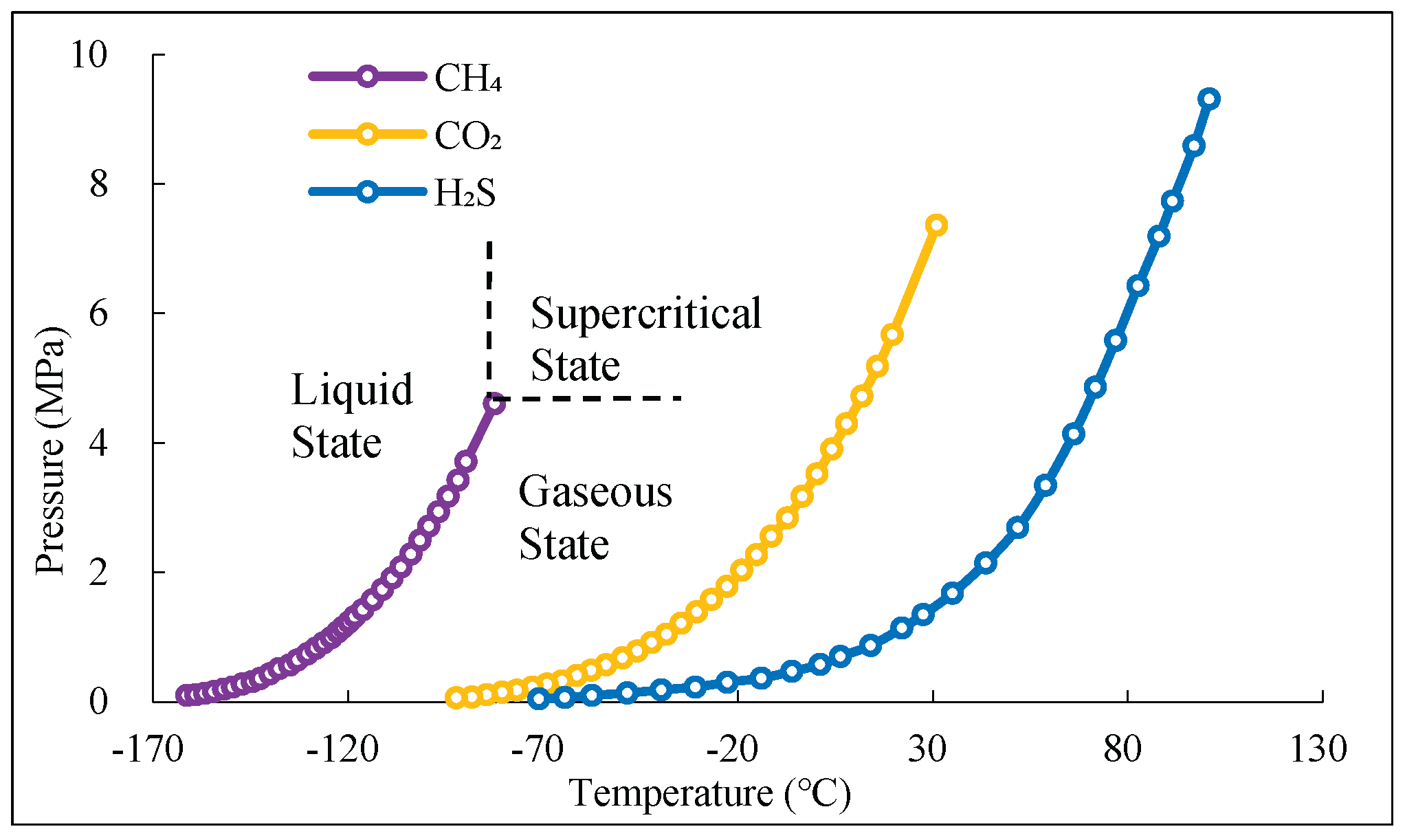
A comparison of the properties of the three gases in Table 2 reveals that the density, viscosity, diffusion coefficient, and thermal conductivity of supercritical fluids lie between those of gaseous and liquid fluids. The density of supercritical fluids is similar to that of liquid fluids, while their viscosity is similar to that of gaseous fluids.
2.2. Pseudo-Critical Point
The pseudo-critical properties of gas mixtures with known components are determined using the calculation method proposed by (WICHERT and AZIZ, 1972) coefficient formula is applied for correction. The pseudo-critical parameters for gases with different components, as calculated, are shown in Table 3. It can be observed that the pseudo-critical points of mixed acidic gases with varying H₂S and CO₂ content differ significantly, and the difference decreases with an increase in CH₄ content.
2.3. Solubility of Acidic Gases
The variation of solubility with well depth is shown in Figure 2.
The drilling fluid formula used in the calculation is: 4% bentonite + (0.2%–0.3%) zwitterionic polymer strong encapsulator + (2%–4%) sulfonated phenolic resin + (2%–4%) lignite resin + (0.4%–0.6%) sodium hydroxide + (3%–5%) sulfonated tannin + (0.3%–0.5%) sodium carbonate + (1%–2%) sulfonated asphalt + (20%–25%) sodium chloride + (0.2%–0.4%) polyanionic cellulose.
As shown in the figure, under the same wellbore temperature and pressure conditions, the solubility of CH₄ is significantly lower than that of CO₂ and H₂S, indicating that CH₄ is almost insoluble in water. Therefore, the effect of CH₄ solubility is neglected when developing the flow model.
3. Acidic Gas Annular Flow Model
An annular flow model for acidic gases is established by considering gas solubility. The basic assumptions of the model are as follows(Alegría et al., 2012):
(1) The fluid flow in the annulus is one-dimensional and continuous.
(2) The inner wall of the annulus is rigid, and complex situations such as abnormal high pressure, lost circulation, and wellbore collapse are not considered.
(3) The fluid invading the wellbore from the formation is gas, with formation water and oil invasion neglected.
(4) Fluids in the annulus do not react with each other; only physical changes occur, with no chemical reactions.
(5) Heat changes caused by fluid phase transitions and the effects of other heat source terms are ignored.
(6) Differences between acidic natural gas mixtures released by drilling fluids and those generated by the reservoir are neglected.
The derivation of the mass and momentum conservation equations, auxiliary equation and boundary conditions of the acid gas annular flow model is shown in Appendix A.
4. Model Solution
The model solving process can be divided into single phase gas blowout model, grid division and constructing difference equation. The detailed derivation process is provided in Appendix B.
4.1. Solution Process
After discretizing the equation, the difference equations between the gas-liquid continuity equation and momentum equation of the acidic gas circulation model are obtained. Use Matlab to solve the model and perform grid division on the 10000 meter well with a grid accuracy of 10m. The differential grid using a four point difference format is gradually solved, as shown in Figure 3. In the figure, "○" is a known parameter and "×" is a parameter to be determined.
Taking the calculation of flow parameters at node 4 in the figure as an example, the detailed calculation process is as follows:
(1) Estimate the pressure value at node 4 ().
(2) Based on the estimated pressure, use the PVT state equation (6) to calculate the gas density at node 4 ().
(3) Estimate the gas content at node 4 ().
(4) Based on the estimated gas content, use the gas and liquid continuity equations (2) and (3) to calculate the gas and liquid flow velocities () and ().
(5) Based on the gas and liquid flow velocities, use the drift flow equation (5) to calculate the actual gas content at node 4 ().
(6) Perform an error analysis on the calculated gas content. If ,,,,then the estimate in step (3) is reasonable, and proceed to the next step.
(7) Otherwise, re-estimate the gas content and repeat the calculations in steps (3) to (6) until the desired accuracy is reached.
(8) Based on the gas-liquid flow velocity and gas content, the pressure at node 4 is calculated using the mixed momentum equation (4). The calculated pressure at node 4 is then compared with the estimated pressure in step (1). If,,,,the estimated pressure is considered reasonable, and the calculation for the node is complete. The flow parameters calculated at the node are then used as the known conditions for the next node. If , the pressure must be re-estimated. The calculation steps should be repeated until the pressure calculation error meets the required (precision.
(9) Repeat this iterative process for the entire time and space domain until the solution for the entire fixed domain is obtained, and the flow parameters at all nodes are determined.
4.2. Model Validation
When acidic gas overflow occurs, due to its inherent toxicity, the risk associated with on-site data collection is high, making the operation challenging. Therefore, this study validates the accuracy of the proposed model by comparing the computational results with previously measured data from overflow wells. Specifically, the work by (Baojiang et al., 2012), which collected data on overflow conditions in wells with high H₂S concentrations across different regions, including key parameters such as annular pressure, mud pit gain, and overflow gas composition. The computational results of this study were compared with these field-measured data, as shown in Figure 4. The comparison results indicate that the trends of the model calculations are largely consistent with the measured data, with a maximum error within ±5%, further demonstrating the high accuracy and reliability of the acidic gas annular flow model developed in this study.
(Aarsnes et al., 2016) simulated the behavior of riser gas under a Rapid Gas Handling (RGH) system, which closes and regulates pressure to 20 bar. A comparison chart (Figure 5) is provided to illustrate the differences between their results and those obtained from the model presented in this study. As shown in the figure, the results obtained from the model in this study closely align with the bubble pressure and ROP pressure predicted by Aarsnes et al.’s model, with a deviation within ±10%. This demonstrates the model’s accuracy and its applicability to practical production calculations.
5. Calculation Example
5.1. Basic Parameters
The Z well of Z oil field is used as the basis for the calculations in this paper. The designed depth of the well is 11,100 meters: the first section depth is 1,500 m, the second section depth is 5,900 m, the third section depth is 8,000 m, the fourth section depth is 10,000 m, and the fifth section depth is 11,100 m. The outer diameter of the annulus is taken as the drill bit diameter (168.3 mm), and the inner diameter of the annulus is taken as the drill collar outer diameter (101.6 mm). During the fifth section, the drill string assembly inside the well consists of:
168.3 mm drill bit + rod drill string (9 m) + float valve (0.5 m) + 127 mm spiral drill collar (189 m) + 101.6 mm heavy drill pipe (144 m) × 101.6 mm inclined drill pipe × S135I (3000 m) + 101.6 mm inclined drill pipe × V150 (2000 m) + 149.2 mm inclined drill pipe × V150I (3057 m) + 149.2 mm inclined drill pipe × V150 (2700 m). The basic input parameters are shown in Table 4.
5.2. Study on the Variation of Acidic Gas Properties with Well Depth
Figure 6 shows the trend of the deviation factor of mixed acidic gases with different compositions as a function of well depth. It can be observed that the deviation factor changes more dramatically near the pseudo-critical point with higher H₂S and CO₂ content, and the minimum value tends to shift towards the wellhead.
From Figure 6(a), the deviation factor of the component with 40% H₂S content changes by more than 0.5, while the deviation factor of the component with 40% CO₂ content also changes dramatically near the pseudo-critical point, but to a lesser extent than that of the component with 40% H₂S content. From Figure 6(b), the component with a higher H₂S content has its minimum deviation factor shifting more to the left, indicating that the higher the H₂S content in the mixed acidic gas, the shallower the well depth at which the minimum deviation factor occurs during ascent along the wellbore.
Figure 7 shows the variation trend of different components of mixed acidic gas properties (density, viscosity) with well depth. From Figure 7(a), the density of mixed gas follows a similar trend to pure CH₄, both increasing with well depth; the rate of increase is initially fast and then slows down. At the same well depth, the density of the mixed gas is significantly greater than that of pure CH₄, and since CO₂ has the highest density among the three gases, the composition with a higher CO₂ content will have a slightly higher density than the one with a higher H₂S content.
From Figure 7(b), it is observed that the viscosity of mixed acidic gas is noticeably higher than that of pure CH₄, and its variation pattern is like that of pure CH₄. Overall, the viscosity of mixed fluid with more CO₂ is slightly higher than that of mixed fluid with more H₂S.
5.3. Migration Pattern of Acidic Gas in the Annular Space
The volume fraction of different components of mixed acidic gas with depth is shown in Figure 8. As seen from Figure 8, below 1500m depth, the volume fraction of different components of mixed acidic gas remains relatively unchanged. However, above 1500m, the volume fraction increases rapidly with decreasing depth.
From Figure 8(a), it can be observed that when the gas reaches the wellhead, the higher the H₂S content in the binary mixed gas, the larger its volume fraction. This indicates that the mixed gas with higher H₂S content experiences more significant volume expansion when it returns to normal conditions. This is because, in the high-temperature and high-pressure environment below 1500m, H₂S is completely dissolved in the drilling fluid, while CH₄ has lower solubility. However, under conditions where temperature and pressure exceed its critical point, CH₄ remains in a supercritical state during the ascent, resulting in a smaller gas-phase volume fraction, less than 0.1. When the depth is less than 1500m, the solubility of H₂S gradually decreases with the reduction in temperature and pressure, leading to its gradual exsolution from the drilling fluid, and the gas volume fraction gradually increases.
From Figure 8(b), it can be observed that the component with higher H₂S content undergoes expansion at a shallower depth and at a faster rate. At the wellhead, the gas-phase volume fraction of the component with higher H₂S content is greater than that of the component with higher CO₂ content. This is because H₂S has a higher solubility than CO₂, and it exsolves later. Additionally, since its deviation factor is smaller than that of CO₂, its volume expansion is more significant.
The variation of flow velocity for different components of mixed acidic gas with well depth is shown in Figure 9. As seen from the figure, the flow velocity of mixed fluid containing acidic gas increases more rapidly near the wellhead, approximately 1 m/s faster than pure CH₄. The mixed phase velocity of the component with higher H₂S content increases slightly later than that of the component with higher CO₂ content, but near the wellhead, the mixed phase velocity increases more rapidly. The reason for this is that the higher the acidic gas content, the smaller the deviation factor in the supercritical state. As temperature and pressure decrease, the gas properties near the critical point change more dramatically.
Figure 10 shows the wellbore pressure variation after the intrusion of two-component mixed acidic gas. From Figure 10(a), the bottom-hole pressure of the well for different mixed acidic gas components sharply decreases with the overflow time. However, the CH₄-H₂S mixed gas experiences a later point of rapid pressure drop and a greater overall pressure drop than the CH₄-CO₂ mixed gas. This is because H₂S has a higher solubility than CO₂, and thus exsolves later in the wellbore. Additionally, due to the smaller deviation factor of the CH₄-H₂S mixture at the critical point compared to the CH₄-CO₂ mixture, gas expansion is more intense at the wellhead, further lowering the liquid column pressure. Therefore, H₂S overflow leads to a larger bottom-hole pressure drop.
Figure 10(b) shows that the overflow annular pressure of the three gas mixtures changes more slowly at greater depths. Near the wellhead, the annular pressure drops gradient increases. This is because the components containing acidic gases reduce the deviation factor at the supercritical point, and as the temperature and pressure near the wellhead decrease, the components with acidic gases expand more intensely, resulting in an intensified overflow and a greater decrease in wellbore pressure.
6. Conclusions
(1) The compressibility factor, density, and viscosity of mixed gases vary with composition and proportion. Higher acidic gas content decreases the compressibility factor while increasing density and viscosity, with more pronounced variations near the pseudo-critical point.
(2) Near the wellhead, natural gas with higher acidic gas content exhibits rapid increases in mixture velocity and gas phase volume fraction due to gas exsolution and expansion. As acidic gas content rises, compressibility decreases significantly in the supercritical state, and gas properties exhibit drastic changes near the critical point.
(3) During upward migration, annular pressure transitions from linear to nonlinear. Higher acidic gas content leads to lower annular pressure at the same depth, attributed to greater solubility in drilling fluids and intensified expansion near the wellhead as temperature and pressure decrease.
(4) Greater acidic gas density results in larger mud pit volume increases. Compared to CO₂-rich gases, H₂S intrusion causes more significant volume expansion due to its lower compressibility factor, leading to greater displacement of drilling fluid near the wellhead.
Nomenclatures
| Symbols | |
| A | Annular cross-sectional area (m2) |
| C0 | Gas distribution coefficient (dimensionless) |
| Cg(T) | The sound velocity of the gas, depending on temperature T (m/s) |
| Cm | Bubble tail velocity (m/s) |
| Eg | Free gas volume fraction (dimensionless) |
| El | Liquid phase volume fraction (dimensionless) |
| Fr | Annular friction (MPa) |
| g | Acceleration of gravity (m/s2) |
| hg | The distance of the bubble head to the top of the riser (m) |
| Mg | Gas mass (kg) |
| mi | Molar concentration of gas i in liquid phase (mol/kg) |
| P | Absolute pressure (MPa) |
| Pc | Gas critical pressure (MPa) |
| Pb | the applied back-pressure (MPa) |
| Pg | the pressure in the gas bubble (assumed uniform) (MPa) |
| Ppr | Quasi critical pressure of gas (MPa) |
| Q0 | The flowrate into the bottom of the riser (m3/s) |
| qg | Gas quality produced per unit depth of reservoir per unit time (kg/(m·s)) |
| R | Molar constant of gas (MPa·1/mol·K) |
| Rls | Solubility of gas in drilling fluid (m3/m3) |
| T | Absolute temperature (K) |
| Tc | Gas critical temperature (K) |
| Tpr | Quasi critical temperature of gas (K) |
| vg | Free gas upward velocity (m/s) |
| vl | Liquid phase reflux velocity (m/s) |
| vrg | Gas-phase drift velocity (m/s) |
| vsg | Gas phase apparent velocity (m/s) |
| vsl | Liquid phase apparent velocity (m/s) |
| v0∞ | Bubble ascent limit speed (m/s) |
| yi | Molar fraction of gas phase (dimensionless) |
| Z | deviation factor (dimensionless) |
| Greek Letters | |
| γ | Activity coefficient (dimensionless) |
| μil(0) | Chemical potential of gas i in liquid phase (dimensionless) |
| μiv(0) | Chemical potential of gas i in the gas phase (dimensionless) |
| ρl | Liquid density (kg/m3) |
| ρg | Free air density (kg/m3) |
| ρpr | Pseudo critical density (kg/m3) |
| ρgs | Gas density under standard conditions (kg/m3) |
| σ | Gas-liquid surface tension (N/m) |
| φi | Fugacity coefficient (dimensionless) |
Funding
All authors certify that they have no affiliations with or involvement in any organization or entity with any financial interest or non-financial interest in the subject matter or materials discussed in this manuscript.
Informed Consent Statement
Informed consent was not applicable for this study.
Conflicts of Interest
The authors declare that they have no potential conflicts of interest, either financial or non-financial, related to this research.
Research Involving Human Participants and/or Animals
This research did not involve human participants or animals.
Appendix A. Acidic Gas Annular Flow Model
Mass and Momentum Conservation Equations
The solubility is calculated using the equation of state method proposed by (Hao et al., 2022; Xiangrui et al., 2023).
where: is the molar concentration of gas i in the liquid phase,,,,; is the mole fraction of gas i in the gas phase, dimensionless; P is the absolute pressure, MPa; T is the absolute temperature, K; is the chemical potential of gas i in the liquid phase; is the chemical potential of gas i in the gas phase; R is the molar gas constant, with a value of ; is the fugacity coefficient, dimensionless; is the activity coefficient, dimensionless.
A physical model, as shown in Figure A-1, is established. Taking the upward flow direction in the annulus as the positive direction, a differential segment dz is analyzed, with a cross-sectional area of A.
Figure 1.
Mass conservation cell physical model.
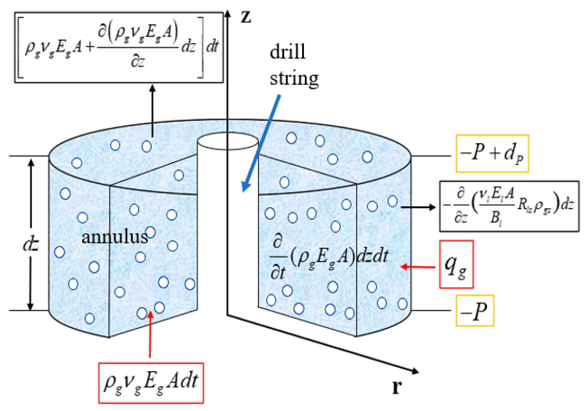
According to the law of mass conservation: Influx Gas + Formation-Generated Gas + Gas Released from Drilling Fluid − Outflow Gas = Total Change. The terms are detailed in Table A1.

Table A1.
Mass components of dz cell.
| Gas Mass Inflow at the Lower Surface | |
| Gas Mass Generated by Formation within the Differential Element | |
| Gas Mass Released from Drilling Fluid within the Differential Element | |
| Free Gas Mass Outflow at the Upper Surface | |
| Total Change within the Differential Element |
Where: A is the cross-sectional area of the annulus, m2; is the density of free gas, ; is the upward velocity of free gas,; is the volume fraction of free gas, dimensionless; is the mass of gas generated by the reservoir per unit depth per unit time,; is the upward velocity of the liquid phase, ; is the volume fraction of the liquid phase, dimensionless; is the solubility of gas in the drilling fluid,; is the density of gas under standard conditions, .
The continuity equation for the mixed acidic gas is:
Similarly, the continuity equation for the liquid phase is:
where: ρl is the density of the liquid phase, .
According to the law of momentum conservation, the combined effects of fluid weight, acceleration, viscous friction between the fluid and the wellbore wall, and momentum exchange between the mixed acidic gas and the drilling fluid within the differential element are balanced, yielding the total momentum equation:
where: Fr is the annular frictional pressure drop, MPa.
Auxiliary Equations and boundary conditions(1) Drift Flux Model Physical Equation:
where: C0 the gas distribution coefficient, dimensionless; vrg is the gas-phase drift velocity, m/s.
(2) Gas Phase Equation of State:
In this equation, Z is the compressibility factor, dimensionless.
(3) Flow Pattern Identification and Friction Calculation:
The flow pattern identification and friction calculation formulas used in this study are shown in Table A2. The specific derivation process and calculation of relevant parameters are introduced in the studies by(Hasan and Kabir, 1988; Hasan and Kabir, 1992).
Table A2.
Flow pattern discriminant and friction calculation formula.
| Flow Pattern | Identification Criterion | Friction Calculation |
| Single-phase Flow | Influx gas completely dissolved | |
| Bubble Flow | ||
| Slug Flow | ||
| Churn Flow | ||
| Annular Flow |
Where: is the apparent velocity of the gas phase, m/s; is the apparent velocity of the liquid phase, m/s; is the bubble rise limit velocity, m/s; is the gas-liquid surface tension, N/m;
(4) Acidic Natural Gas Compressibility Factor
The method used when the pressure is less than 35 MPa and greater than or equal to 35 MPa is shown in Table A3.
Table A3.
Calculation formula of compression coefficient of acid natural gas.
| Pressure | The calculation formulas |
Where: is the critical temperature of the gas, K; is the critical pressure of the gas, MPa; is the pseudo-critical temperature of the gas, K; is the pseudo-critical pressure of the gas, MPa; is the pseudo-critical density of the gas, kg/m3.
The initial conditions refer to the fluid flow state and pressure distribution in the annulus at the initial moment. When there is no acidic gas invasion into the annulus at t=0, the fluid in the annulus is a single-phase flow. The flow state and pressure distribution in the annulus at any given time are determined by the boundary conditions. The initial conditions and boundary conditions are shown in Table A4.
Table A4.
Initial and boundary conditions.
| Initial Conditions | Boundary Conditions |
Where: P(t, N) is the pressure at the wellhead node, MPa.
Appendix B. Derivation of Governing Equations for Model Solution
- (1)
- Single-Phase Gas Blowout Model
Considering a single bubble representation of gas in a riser, the pressure in the gas relates to the gas volume as:
where: Mg is the gas mass and Cg(T) is the sound velocity of the gas, depending on temperature T.
Consider a control volume covering the gas bubble and an incompressible liquid column above. Setting the liquid velocity equal to the head of the gas bubble, we can employ a momentum balance the gas and liquid of the control volume to get:
where: hg is the distance of the bubble head to the top of the riser, m; Pg is the pressure in the gas bubble (assumed uniform), MPa; Pb is the applied back-pressure (equal to atmospheric when no riser gas handler is used), MPa; g is the acceleration of gravity, m/s2.
Expressing the gas volume rate of change as the difference in velocity between the bubble head vG and tail Cm we get the system of equations.
And the closure relations:
where: Q0 is the flowrate into the bottom of the riser.
We note that the mode associated with the acceleration, equation (B-1), would be expected to have a large eigenvalue (meaning it tends rapidly to its equilibrium) due to acceleration terms tending to be small is such a context. The consequence is that the system may become stiff, and some care must be taken in implementation. Immediate equilibrium could be imposed on (B-1) to avoid this, and without expecting significant loss of accuracy, however, we will avoid doing this as the resulting expression becomes quite involved.
Finally, using to denote the position of the tail of the gas bubble, we can write the pressure at the BOP as:
- (2)
- Grid Division.
The spatial domain is divided using a fixed-step grid division method. The step size and total number of spatial grids in the defined domain are given by:
where: .
For the time domain, non-uniform step sizes can be used by dividing the spatial grid step size by the current grid fluid velocity. The step size for each time grid and the total number of time grids are given by:
where: .
- (3)
- The difference equation
Difference equation for the gas phase continuity equation:
Difference equation for the liquid phase continuity equation:
Momentum equation
The difference format for the momentum equation is:
where:
- (4)
- Boundary conditions
The discretization of the initial conditions and boundary conditions is shown in Table A5.
Table A5.
Dispersion of initial conditions and boundary conditions.
| Dispersion of initial conditions | boundary conditions |
References
- Aarsnes, U.J., Hauge, E. and Godhavn, J.-M., 2016. Mathematical Modeling of Gas in Riser, SPE Deepwater Drilling and Completions Conference.
- Al-Kayiem, H.H., Osei, H., Hashim, F.M. and Hamza, J.E., 2019. Flow structures and their impact on single and dual inlets hydrocyclone performance for oil–water separation. Journal of Petroleum Exploration and Production Technology, Vol.9(No.4): 2943-2952. [CrossRef]
- Al-Safran, E., Ghasemi, M. and Al-Ruhaimani, F., 2020. High-Viscosity Liquid/Gas Flow Pattern Transitions in Upward Vertical Pipe Flow. SPE Journal, Vol.25(No.3): 1155-1173. [CrossRef]
- Alegría, L.M. et al., 2012. Friction Factor Correlation for Viscoplastic Fluid Flows through Eccentric Elliptical Annular Pipe, IADC/SPE Asia Pacific Drilling Technology Conference and Exhibition.
- Baojiang, S., Rongrong, S. and Zhiyuan, W., 2012. Overflow behaviors of natural gas kick well with high content of H2S gas. Journal of China University of Petroleum(Edition of Natural Science), 36(01): 73-79.
- Baojiang, S. et al., 2020. Application and prospect of the wellbore four-phase flow theory in the field of deepwater drilling and completion engineering and testing. Natural Gas INdustry, 40(12): 95-105.
- Chengzao, J., Lin, J. and Wen, Z., 2025. Tight oil and gas in Whole Petroleum System: accumulation mechanism. enrichment regularity,and resource prospect. Acta Petrolei Sinica, 46(01): 1-16+47.
- Dou, L. et al., 2012. Study on the well control safety during formation high-sulfur gas invasion.
- Faluomi, V., Bonizzi, M. and Ghetti, L., 2017. Development and Validation of a Multiphase Flow Simulator. (TEA Sistemi SpA) (TEA Sistemi SpA) (TEA Sistemi SpA) (TEA Sistemi SpA).
- Feng, G., Changqing, J. and Hong, L., 2023. Key technologies for safe and efficient development and long-term stable production of the Luojiazhai high-sulfur gas field in the Sichuan Basin. Natural Gas Industry, 43(09): 85-92.
- Ferroudji, H. et al., 2021. Study of Ostwald-de Waele fluid flow in an elliptical annulus using the slot model and the CFD approach. Journal of Dispersion Science and Technology, 42(9): 1395-1407. [CrossRef]
- Guo, G. et al., 2025. A review of Wellhead pressure reduction methods in hydraulic fracturing. Journal of Petroleum Exploration and Production Technology, 15(6): 106. [CrossRef]
- Hao, T. et al., 2022. Design method and application of accurate adjustment scheme for water injection wells around adjustment wells. Journal of Petroleum Exploration and Production Technology, Vol.12(No.3): 743-752. [CrossRef]
- Hasan, A.R. and Kabir, C.S., 1988. Predicting Multiphase Flow Behavior in a Deviated Well. (U. of North Dakota);(Schlumberger Well Services), Vol.3(No.4): 474-482. [CrossRef]
- Hasan, A.R. and Kabir, C.S., 1992. 2-PHASE FLOW IN VERTICAL AND INCLINED ANNULI. Department of Chemical Engineering, University of North Dakota, Grand Forks, ND 58202, United States;Chevron Oil Field Research Co., La Habra, CA 90633, United States, Vol.18(No.2): 279-293. [CrossRef]
- Hua, J. et al., 2022. Process and model of hydrocarbon accumulation spanning major tectonic phases of Sinian Dengying Formation in the Sichuan Basin. Natural Gas Industry, 42(05): 11-23.
- Jiangfei, L. et al., 2016. Pipeline transport containing impurity CO2. Science and technology Guide, 34(02): 173-177.
- Kiran, R., Salehi, S., Mokhtari, M. and Kumar, A., 2019. Effect of Irregular Shape and Wellbore Breakout on Fluid Dynamics and Wellbore Stability, 53rd U.S. Rock Mechanics/Geomechanics Symposium.
- Krishna, S. et al., 2020. Explicit flow velocity modelling of yield power-law fluid in concentric annulus to predict surge and swab pressure gradient for petroleum drilling applications(Article). State Key Laboratory of Petroleum Resources and Prospecting, China University of Petroleum, Beijing, 102249, China; College of Geosciences, China University of Petroleum, Beijing, 102249, China; Strategic Res, Vol.195: 107743. [CrossRef]
- Qian, L. et al., 2023. The characteristics of solid sulfur deposition in high sulfur gas reservoir. Fault-Block Oil & Gas Field, 30(06): 999-1006.
- Shaomu, W. et al., 2024. Key technological innovation and successful practice in safe and highly-efficient development of ultra-high sulfur monoblock gas fields in the Sichuan Basin. Natural Gas Industry, 44(11): 37-49.
- Shihui, S., Wen, X., Jinyu, F. and Haiyan, T., 2019. An Analysis on Flow Characteristics of Foam Drilling under Formation Fluid Intrusion Conditions. CHINA'S MANGANESE INDUSTRY, 37(06): 42-47.
- Sun, B. et al., 2018. Multiphase flow behavior for acid-gas mixture and drilling fluid flow in vertical wellbore. State Key Laboratory of Petroleum Resources and Prospecting, China University of Petroleum, Beijing, 102249, China; College of Geosciences, China University of Petroleum, Beijing, 102249, China; Strategic Res, Vol.165(No.0): 388-396. [CrossRef]
- Tang, M., He, L., Kong, L., He, S. and Zhang, T., 2022a. Simplified modeling of laminar helical flow in eccentric annulus with YPL fluid. Energy Sources Part a-Recovery Utilization and Environmental Effects, 44(1): 2061-2074. [CrossRef]
- Tang, M. et al., 2022b. Gravity displacement gas kick law in fractured carbonate formation. Journal of Petroleum Exploration and Production Technology, Vol.12(No.11): 3165-3181. [CrossRef]
- Wang, F. et al., 2024. Upper limit estimate to wellhead flowing pressure and applicable gas production for a downhole throttling technique in high-pressure–high-temperature gas wells. Journal of Petroleum Exploration and Production Technology, 14(6): 1443-1454.
- Wang, Z., Sun, B. and Sun, X., 2016. Calculation of Temperature in Fracture for Carbon Dioxide Fracturing. SPE JOURNAL, Vol.21(No.5): 1491-1500. [CrossRef]
- Weiner et al., 2017. Annular phase behavior analysis during marine natural gas hydrate reservoir drilling. Acta Petrolei Sinica, 38(06): 710-720.
- Wezehwa, Jin, Z. and Tinghu, W., 2018. Safety planning analysis of natural gas Wells containing hydrogen sulfide. China Petroleum and chemical standards and quality, 38(07): 83-84.
- WICHERT, E. and AZIZ, K., 1972. CALCULATE Z S FOR SOUR GASES. Hydrocarbon Processing, Vol.51(No.5): 119.
- Xiangrui, C., Yunpeng, W., Zhihua, H. and Qiaohui, F., 2023. Solubility models of CH4, CO2 and noble gases and their geological applications. Natural Gas Geoscience, 34(04): 707-718.
- Xin, L., Shiming, H., year, S.s., Yong, S. and Lanfeng, Y., 2016. Transient flow simulation of gas-liquid two-phase flow in wellbore based on AUSMV algorithm. World scientific and technological research and development, 38(06): 1170-1176.
- Xinming, W. et al., 2018. Resistance characteristics of supercritical CO2 in a circular tube. CIESC Journal, 69(12): 5024-5033.
- Xinyu, G. et al., 2024. Prediction and Application of Pore Pressure for Carbonate Reservoirs in Zhongjiang–Penglai of China, SPE Caspian Technical Conference and Exhibition.
- Yuanyuan, M., 2019. Raman spectroscopy of H2S dissolution process in H2S-H2O-nacl system. Master Thesis.
- Yuyu, X. et al., Geochemical characteristics of bitumen in ancient oil and gas reservoirs in the north-northwest margin of Sichuan Basin are indicative of lead-zinc deposit enrichment. Bulletin of Mineralogy, Petrology and Geochemistry: 1-17.
- Zaidin, M.F., Kantaatmadja, B.P. and Chapoy, A., 2019. Experimental Study to Estimate CO2 Solubility in a High Pressure High Temperature HPHT Reservoir Carbonate Aquifer.
- Zainith, P. and Mishra, N.K., 2021. A Comparative Study on Thermal-Hydraulic Performance of Different Non-Newtonian Nanofluids Through an Elliptical Annulus. Journal of Thermal Science and Engineering Applications, 13(5). [CrossRef]
- Zhou, H., Fan, H., Wang, H., Niu, X. and Wang, G., 2018. A Novel Multiphase Hydrodynamic Model for Kick Control in Real Time While Managed Pressure Drilling, SPE/IADC Middle East Drilling Technology Conference and Exhibition.
Figure 2.
Solubility of the three gases under wellbore temperature and pressure conditions.
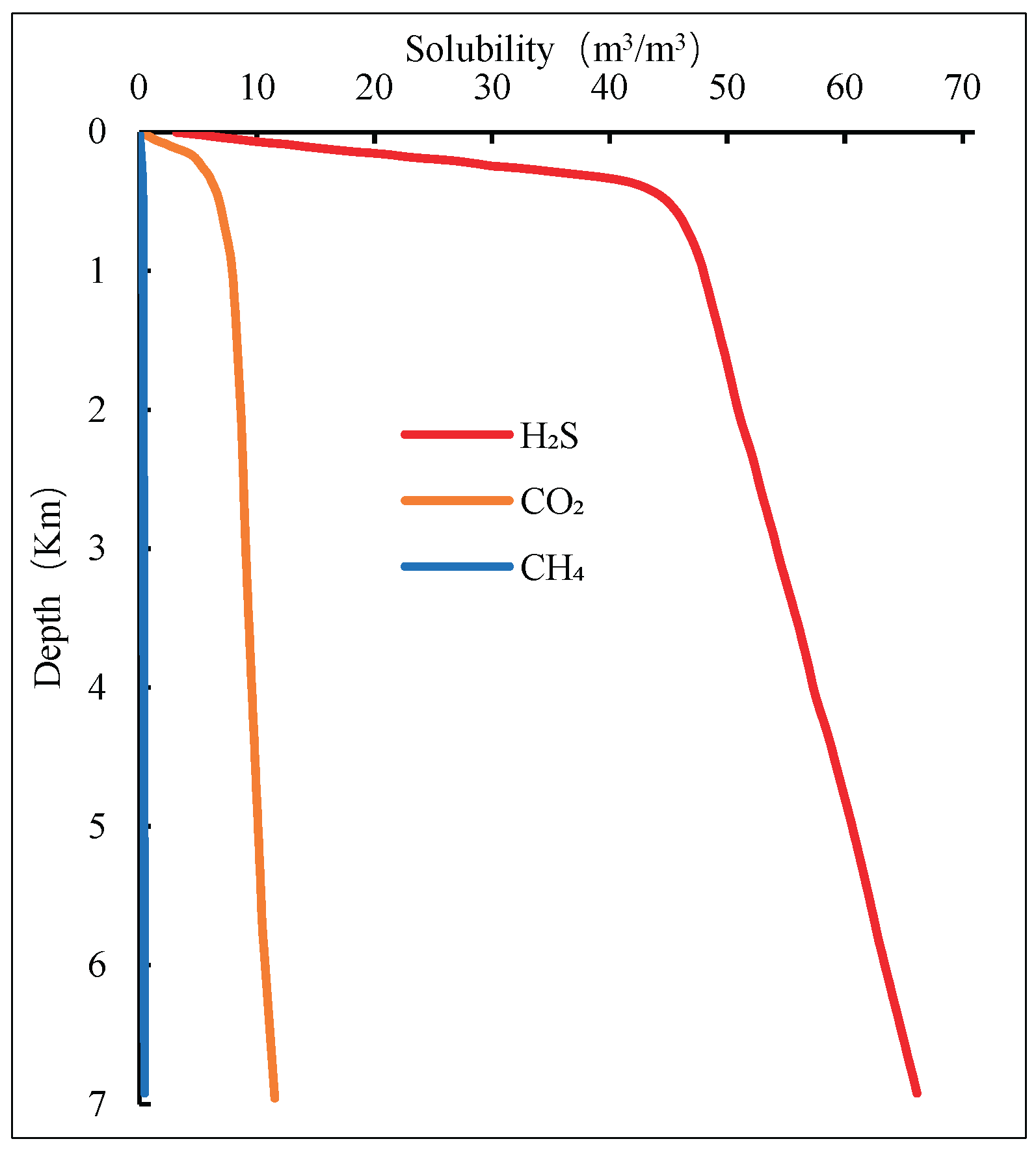
Figure 3.
Grid division diagram of four-point difference scheme.
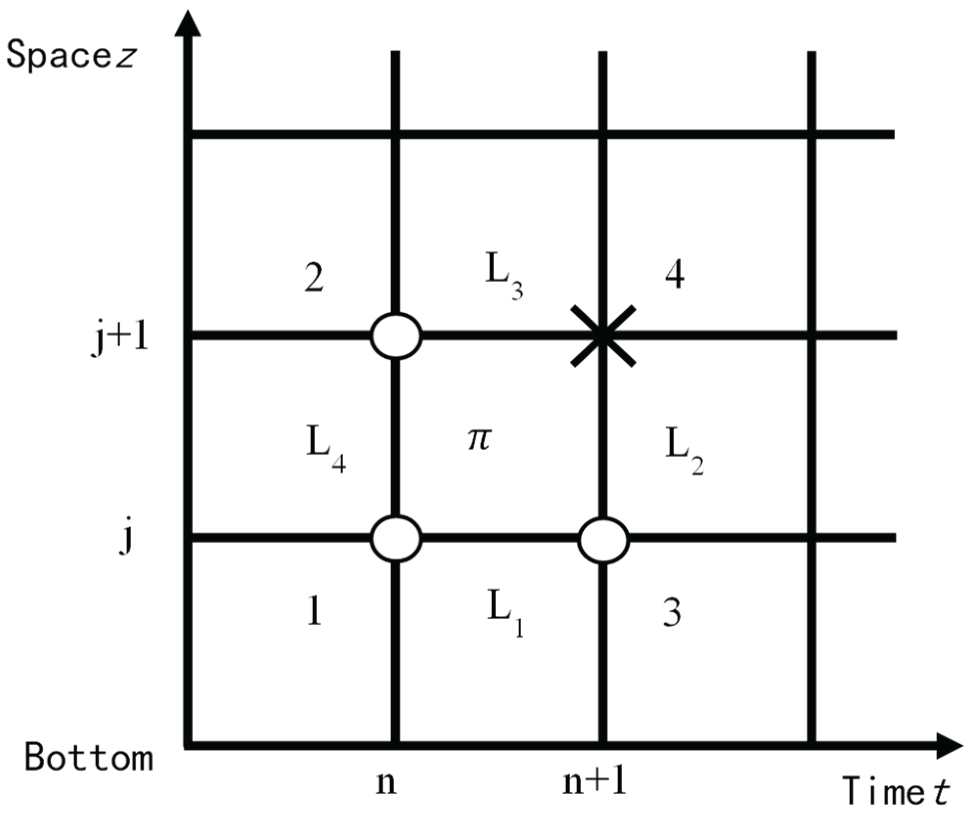
Figure 4.
Comparison and verification: (a) annulus pressure; (b) Increment of mud pool.
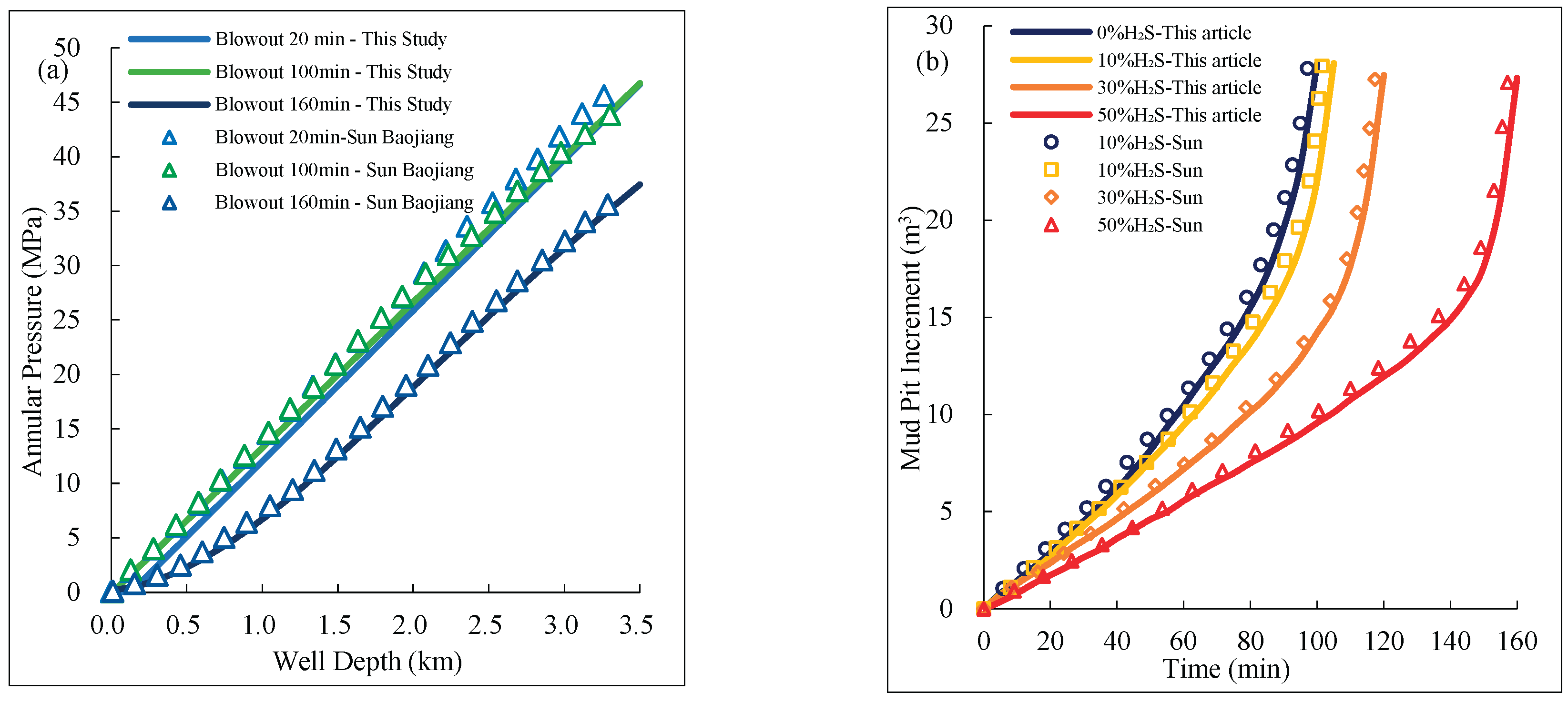
Figure 5.
Comparison between the calculation results of (Aarsnes et al., 2016) and those of the model proposed in this study.
Figure 5.
Comparison between the calculation results of (Aarsnes et al., 2016) and those of the model proposed in this study.
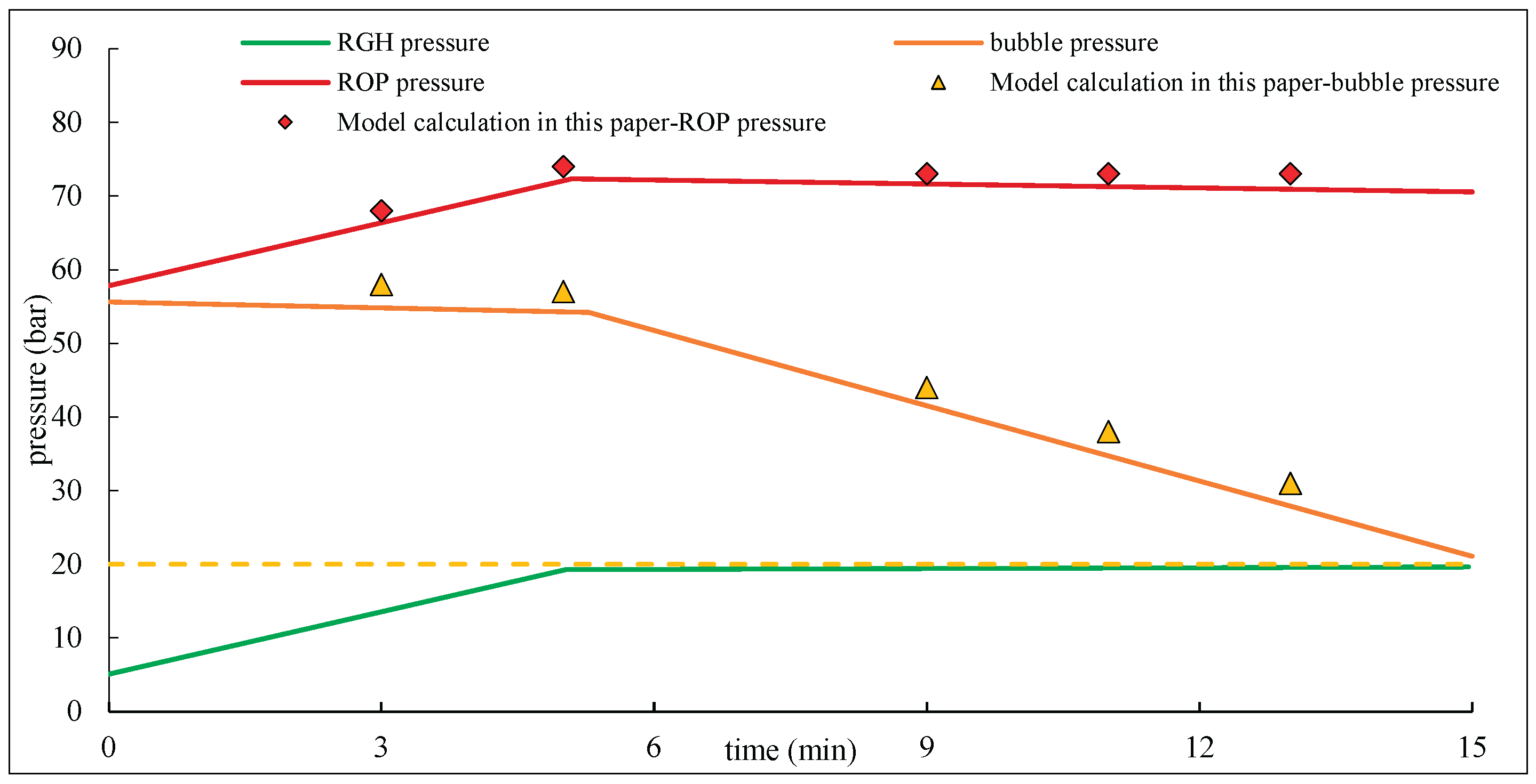
Figure 6.
Deviation factors of acidic gas mixed with different components: (a) Acidic gas mixed with two components; (b) three-component acid gas mixture.
Figure 6.
Deviation factors of acidic gas mixed with different components: (a) Acidic gas mixed with two components; (b) three-component acid gas mixture.
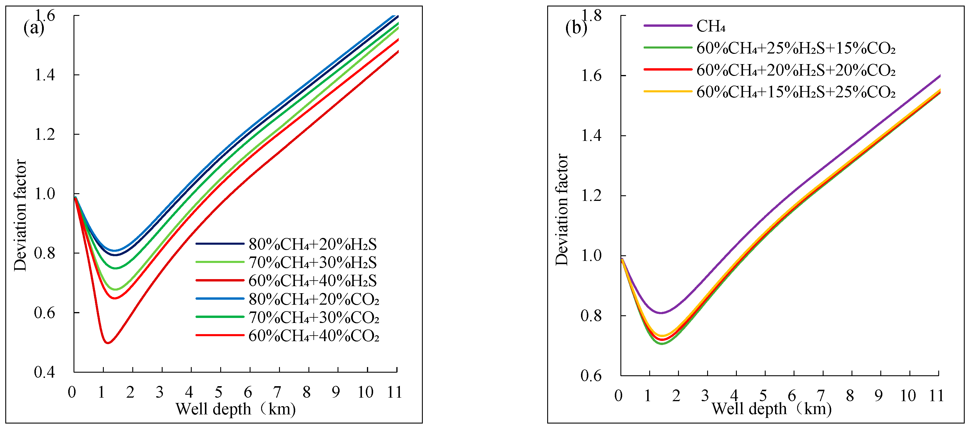
Figure 7.
Characteristics of acidic gas mixed with different components: (a) density;(b) Viscosity.
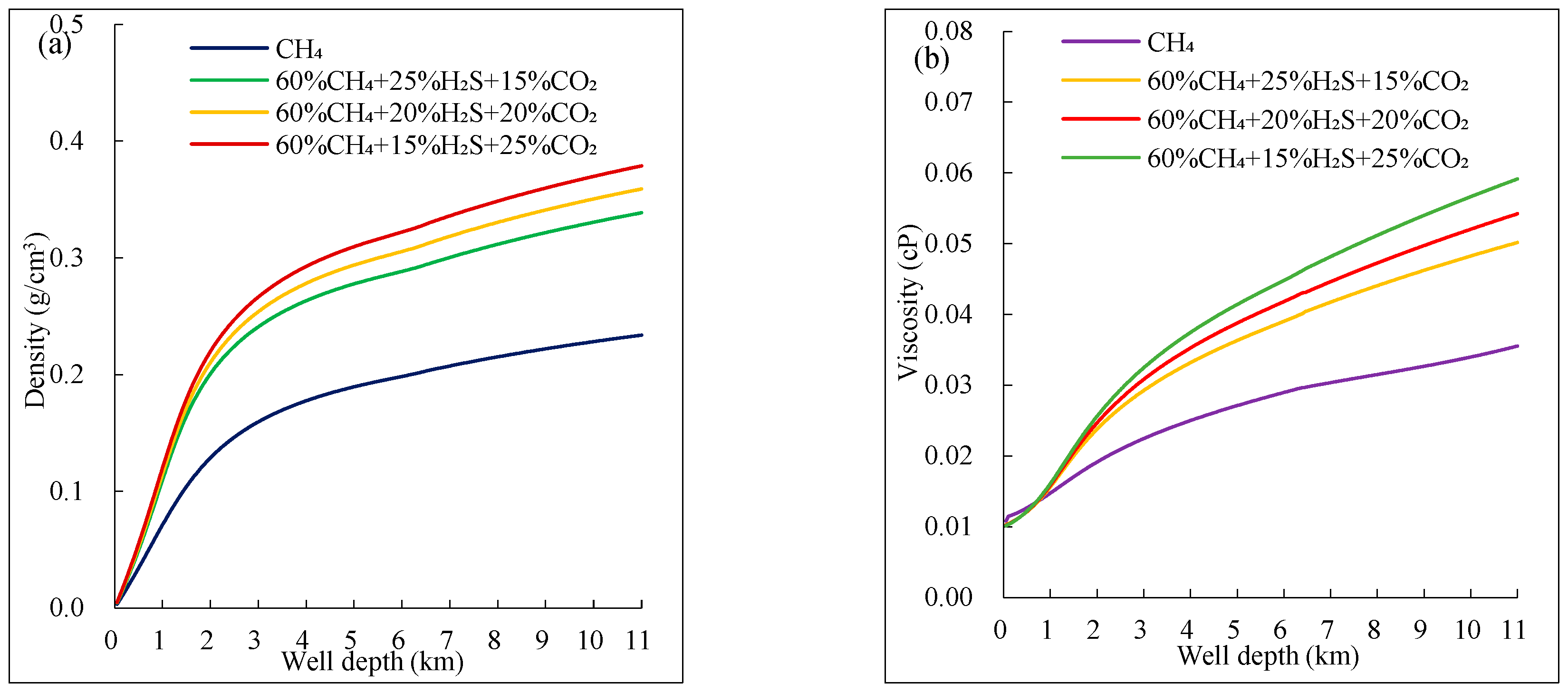
Figure 8.
Volume fraction of acidic gas mixed with different components: (a) two-component acidic gas mixed;(b) three-component acid gas mixture.
Figure 8.
Volume fraction of acidic gas mixed with different components: (a) two-component acidic gas mixed;(b) three-component acid gas mixture.
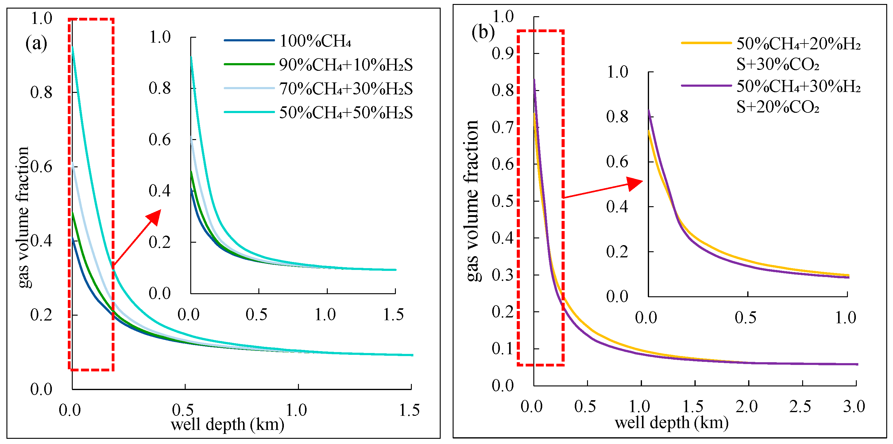
Figure 9.
Flow rate of acidic gas mixed with different components.
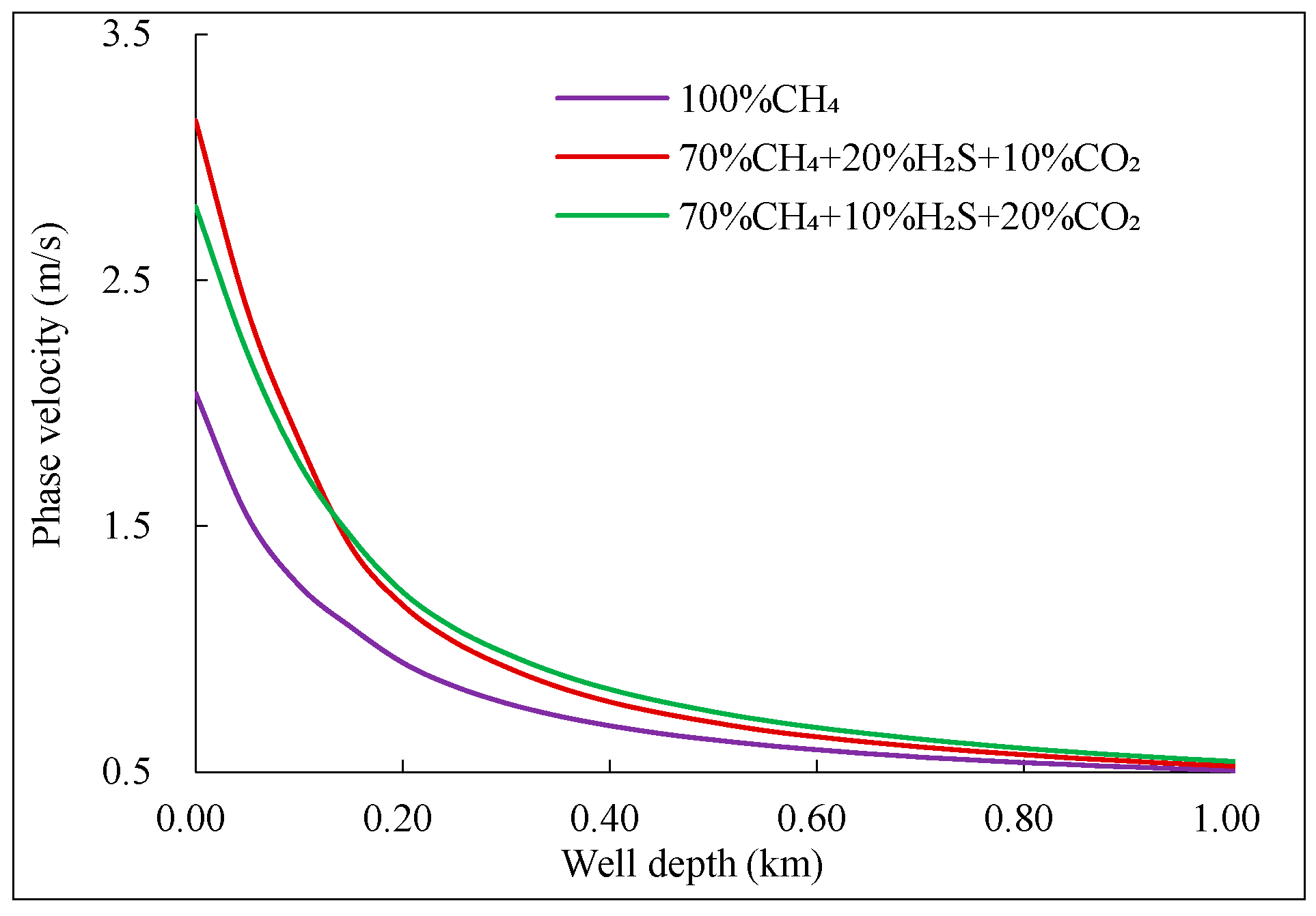
Figure 10.
Change of wellbore pressure after intrusion of two-component mixed acid gas: (a) bottom-hole pressure;(b) Wellbore pressure.
Figure 10.
Change of wellbore pressure after intrusion of two-component mixed acid gas: (a) bottom-hole pressure;(b) Wellbore pressure.
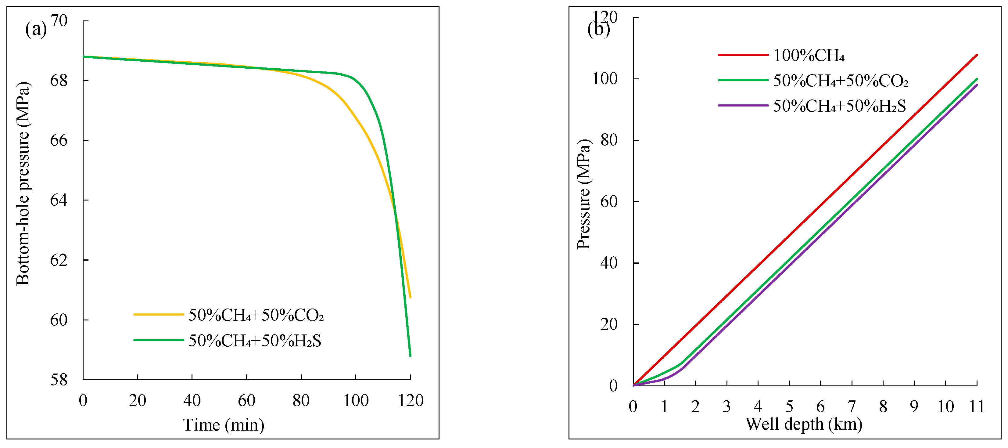
Table 1.
Acid gas deep well blowout statistics.
| Well Number. | Time | Depth (m) |
Formation | Ejected Medium | H₂S Content (g/m3) |
CO₂ Content (g/m3) | Casualties (people) |
| Luojia 16H | 2003.12 | 4050 | Feixianguan Formation | Gas | 151.0 | -- | 243 |
| Tazhong823 | 2005.12 | 5550 | Ordovician | Oil and Gas | 22.0 | -- | |
| Luojia 2 | 2006.03 | 3404 | Feixianguan Formation | Gas | 125.5 | 106.88 | |
| Zhonggu70 | 2018.03 | 7413 | Yingshan Formation | Oil and Gas | 4000 | -- | |
| Tazhong 726-2X | 2018.12 | 5594 | Ordovician | Gas | 500-4800 | -- |
Table 2.
Compares the characteristics of different state bodies.
| Fluid types | Density(kg/m3) | Viscosity(Pa·s) | Diffusion coefficient(m2/s) | hermal conductivity(W/m·k) |
| Gas | 1 | 1~3×10⁻⁵ | 5~200×10-6 | 5~30×10-3 |
| Supercritical fluid | 200~700 | 2~10×10-4 | 0.01~1×10⁻⁶ | 30~70×10-3 |
| Liquid | 1000 | 1~10×10-2 | 0.4~3×10⁻⁹ | 70~250×10-3 |
Table 3.
Quasi-critical parameters of gas mixtures of different components.
| Gas Composition | Pseudo-Critical Temperature (°C) | Pseudo-Critical Pressure (MPa) | |
| Binary Mixture | -15.47 | 2.14 | |
| -51.16 | 2.90 | ||
| -78.56 | 4.66 | ||
| -44.84 | 5.51 | ||
| -67.51 | 4.96 | ||
| -82.87 | 4.59 | ||
| Ternary Mixture | -57.32 | 5.12 | |
| -60.31 | 5.08 | ||
| -63.19 | 5.01 | ||
Table 4.
Basic input parameters.
| Parameters | Values | Parameters | Values |
| Relative density of H₂S | 1.189 kg/m3 | Drilling fluid replacement | 0.012 m³/s |
| Relative density of CO₂ | 1.535 kg/m3 | Formation temperature gradient | 0.03 ℃/m |
| Relative density of natural gas | 0.717 kg/m3 | Surface temperature | 20 ℃ |
| Viscosity of drilling fluid | 0.04 Pa·s | Surface pressure | 0.1 MPa |
| Density of drilling fluid | 1510 kg/m3 | Kick flow rate | 0.5 m³/s |
| Formation pressure gradient | 0.012 MPa/m |
Disclaimer/Publisher’s Note: The statements, opinions and data contained in all publications are solely those of the individual author(s) and contributor(s) and not of MDPI and/or the editor(s). MDPI and/or the editor(s) disclaim responsibility for any injury to people or property resulting from any ideas, methods, instructions or products referred to in the content. |
© 2025 by the authors. Licensee MDPI, Basel, Switzerland. This article is an open access article distributed under the terms and conditions of the Creative Commons Attribution (CC BY) license (http://creativecommons.org/licenses/by/4.0/).
Copyright: This open access article is published under a Creative Commons CC BY 4.0 license, which permit the free download, distribution, and reuse, provided that the author and preprint are cited in any reuse.


