
Submitted:
21 July 2025
Posted:
23 July 2025
You are already at the latest version
Abstract
Background: This research investigates the application of Artificial Intelligence (AI), particularly biomimetic convolutional neural networks (CNNs), for the automatic classification of gastrointestinal (GI) polyps in endoscopic images. The study combines AI and Transfer learning techniques to support early detection of colorectal cancer by enhancing diagnostic accuracy with pre-trained models. Methods: The Ksavir dataset, comprising 4,000 annotated endoscopic images across eight polyp categories, was used. Images were pre-processed via normalisation, resizing and data augmentation. Several CNN architectures—including state-of-the-art optimized ResNet50, DenseNet121, MobileNetV2, and others—were trained and evaluated. Models were assessed through training, validation, and testing phases, using performance metrics such as overall accuracy, confusion matrix, precision, recall, and F1 score. Results: ResNet50 achieved the highest validation accuracy at 90%, followed closely by DenseNet121 with 87.5% and MobileNetV2 with 86.5%. The models demonstrated good generalisation, with small differences between training and validation accuracy. Average inference time was under 0.5 seconds on a computer with limited resources, confirming real-time applicability. Confusion matrix analysis indicates common errors frequently occurred between visually similar classes, particularly when reviewed by less-experienced medical physicians. These errors underscore the difficulty of distinguishing subtle features in gastrointestinal imagery and highlight the value of model-assisted diagnostics in supporting clinical decision-making. Conclusions: This obtained results confirms that Deep learning-based CNN architectures, combined with Transfer learning and optimisation techniques, can classify accuratly endoscopic images and support medical diagnostics. Recommended solutions to address classification challenges included the use of advanced data augmentation strategies, such as rotation, flipping, contrast adjustment, and scaling—to artificially increase dataset diversity and improve model generalisation. Additionally, explainability techniques were applied, most notably Gradient-weighted Class Activation Mapping (Grad-CAM), which generates visual heatmaps to highlight the regions within an image that influenced the model’s prediction. These methods help identify potential sources of error and improve transparency, making CNN-based decision systems more interpretable for clinicians.
Keywords:
human brain
; artificial neural network
; biomimetic algorithm
; medical imaging
; computational hard problem
; gastrointestinal polyps
; machine learning
; deep neural network
; colorectal disease
1. Introduction
Colorectal cancer (also known as colon or rectal cancer) [1] is one of the most common causes of death worldwide, and detecting gastrointestinal (GI) polyps plays an important role in its prevention [2,3]. With the rapid advancement of Artificial Intelligence (AI) and neural networks, the application of these technologies in the medical field is becoming increasingly promising.
Certain GI polyps, particularly adenomatous and serrated types, carry a risk of progressing to cancer if not identified and removed in time. Regular screening and timely intervention are essential to reduce the likelihood of malignant transformation [4].
Therefore, integrating AI into diagnostic processes can provide significant support for physicians, enabling them to identify errors more quickly and accurately. The goal is not to replace human expertise but to complement it by providing specialists with modern tools that enhance their work and reduce human error rates [5].
Compared to classical Machine Learning (ML) methods [6,7,8], which perform well with structured and diverse datasets, Deep Learning (DL) architectures [9], like artificial neural networks, are themselves biomimetic in nature, modeled after the human brain’s layered processing, making them powerful for interpreting biological data in domains such as medical image diagnostics or facial recognition [10].
Artificial Neural Networks (ANNs) [11] are an important subset of ML algorithms, inspired by the structure and functioning of the human brain [12]. They consist of layers of artificial neurons that process data through weighted connections, allowing the system to learn and generalize from complex data.
Convolutional Neural Networks (CNNs) [13] are a specialized category of artificial neural networks, primarily used in image processing and automatic visual pattern recognition. These networks are inspired by how the human brain processes visual information, enabling them to learn spatial and hierarchical features from raw images [14,15].
A CNN structure includes several types of layers: convolutional layers, activation layers (e.g., ReLU), pooling layers (e.g., max-pooling), followed by one or more fully connected layers. Convolutional layers apply filters (kernels) over images, automatically extracting important features such as edges, complex shapes, or text regions [16].
CNNs have rapidly evolved due to their ability to automatically extract visual features without human intervention. Initially, models like Alex Convolutional Neural Network (AlexNet) [15], Visual Geometry Group Network (VGGNet) [16], and Inception Network by Google (GoogleNet) [17] were used for simple binary classification tasks.
Later, deeper networks such as Residual Network (ResNet) [18] and Densely Connected Convolutional Network (DenseNet) [19] significantly improved the classification [20], detection, and segmentation of brain lesions, including gliomas, meningiomas and tumors, in multimodal Magnetic Resonance Imaging (MRI) scans such as T1-weighted, T2-weighted, Fluid Attenuated Inversion Recovery (FLAIR), and contrast-improved sequences.
Recent research has focused on hybrid neural architectures such as Convolutional Neural Network-Long Short-Term Memory (CNN-LSTM) models, which combine spatial feature extraction with temporal pattern recognition [13,21,22]. These models are particularly effective in medical imaging tasks where both spatial and sequential data characteristics are present. Transfer learning techniques have also gained traction, leveraging pre-trained models like VGGNet, ResNet, and Inception trained on large-scale datasets such as ImageNet (over 14 million images) [23,24] and adapting them to smaller medical datasets, often containing fewer than 10.000 annotated images. This approach obtained improvements in classification accuracy, sensitivity, and specificity, especially in tasks like brain tumor grading, breast cancer subtype identification, and lesion segmentation in MRI and histopathology images [25].
In medical imaging, transparency in AI decisions is crucial. Explainable Artificial Intelligence (XAI) techniques such as Gradient-weighted Class Activation Mapping (Grad-CAM), Local Interpretable Model-Agnostic Explanations (LIME), and SHapley Additive exPlanations (SHAP) enable visualization of image regions that significantly influence model predictions, helping radiologists interpret how decisions are made [26]. The study [11] contributes to the evolving field of AI-driven medical image analysis by systematically comparing multiple CNN architectures, both classical and advanced, including Capsule Network (CapsNet), FastAI-based models. These architectures are applied to a specialized endoscopic image dataset. Studies highlight the applicability of Grad-CAM in localizing suspicious lesions in mammograms or Computed Tomography (CT) scans [20], while LIME and SHAP have been successfully used in predicting COVID-19 severity from lung radiographs [7].
Numerous studies have demonstrated the efficiency of CNNs in medical image analysis, especially in detecting and classifying anomalies in endoscopic procedures [6]. For instance, a recent study [27] introduced the Ksavir dataset and evaluated several automatic classification methods for GI images, providing an essential starting point for performing researches.
This research presents an integrative deep learning framework of advanced CNN architectures for the automatic classification of gastrointestinal lesions from endoscopic images. The proposed methodology integrates biomimetic modeling with Explainable Artificial Intelligence (XAI) techniques, including Grad-CAM, LIME, and SHAP.
The architectures evaluated in this work include classical models such as AlexNet and VGGNet, as well as more advanced frameworks like GoogLeNet (Inception Network), ResNet (Residual Network), DenseNet (Densely Connected Convolutional Network), and CapsNet (Capsule Network). These models were benchmarked using the Ksavir dataset [27] and Transfer learning is employed to adapt large-scale pre-trained models. The classes used represent a mix of anatomical landmarks, pathological findings, and procedural outcomes and are defined as follows:
- Dyed-lifted-polyps: Images showing polyps that have been stained and elevated using submucosal injection, aiding in visual contrast and resection planning.
- Dyed-resection-margins: Post-polypectomy images highlighting the margins of resected areas, stained to assess completeness of removal.
- Esophagitis: Inflammatory lesions of the esophageal mucosa, often appearing as erythematous streaks or erosions near the Z-line.
- Polyps: Unstained mucosal protrusions, typically benign growths that may serve as precursors to colorectal cancer.
- Ulcerative-colitis: Chronic inflammatory changes in the colon, characterized by mucosal ulceration, granularity, and vascular pattern loss.
- Normal-cecum: Anatomical landmark at the beginning of the large intestine, often used to confirm complete colonoscopy.
- Normal-pylorus: The muscular opening between the stomach and duodenum, appearing as a round, symmetric structure in healthy individuals.
- Normal-z-line: The gastroesophageal junction, where the squamous epithelium of the esophagus transitions to the columnar epithelium of the stomach.
The novelty of this study lies in its biomimetic approach to model selection, wherein biologically inspired design principles, such as hierarchical layer organization and local feature abstraction, are used to evaluate and compare advanced CNN architectures. The goal is to identify the most computationally model for the automatic classification of gastrointestinal lesions in endoscopic images, as applied to the Ksavir dataset.
The main contributions of this study to the state-of-the-art in medical image classification are as follows:
- Benchmarking of CNN Architectures: A set of CNN models, including classical architectures like AlexNet and VGGNet, and advanced designs such as GoogLeNet (Inception), ResNet, DenseNet, and CapsNet were tested on the Ksavir dataset [27], composed of real-world endoscopic images, to assess their effectiveness in gastrointestinal lesion categorization.
- Optimizations: DenseNet121 and ResNet50 were fine-tuned using Transfer learning and dynamic class weighting, while CapsNet was improved with attention mechanisms to improve feature localization and reduced overfitting, especially in classes with limited samples. Thus, choosing ResNet50 represents a contribution of this study, guided by both optimization parameter tuning and empirical performance metrics, including validation accuracy and loss behavior across multiple folds.
- Biomimetic Model Selection: The study introduces a biomimetic framework for selecting CNN architectures, inspired by the hierarchical and layered processing of the human visual cortex [14]. This approach guided the prioritisation of models that emulate biological feature abstraction, such as residual and capsule-based networks.
- Explainability Integration: To improve performance on sparse and imbalanced medical datasets, this study combines Explainable Artificial Intelligence (XAI) techniques, namely Grad-CAM, LIME, and SHAP with Transfer learning from large-scale datasets such as ImageNet. The novelty lies in the task-specific adaptation of XAI methods to guide model and error analysis, enabling iterative feedback during training.
- Benchmarking: The comparative analysis between ResNet50, DenseNet121, and MobileNetV2 offered the best trade-off between accuracy, inference speed, and generalisation. In contrast, deeper models such as NASNetLarge and EfficientNetB8 showed signs of overfitting and slower inference.
The structure of the work is divided into five chapters. Section 1 provides a general introduction to the topic, explains why the subject was chosen, and presents the current context of AI in the medical field. It also describes general objectives, methodology, and dataset used. Section 2 covers theoretical foundations of machine learning and neural networks, focusing on CNNs and Transfer learning, with details on the CNN architectures used, describes their selection process, and mentions models excluded after preliminary testing. It also explains the research methodology, dataset, experimental stages, infrastructure, and applied evaluation methods. Section 3 presents accuracy and loss graphs for each tested CNN architecture. These graphs illustrate the model’s behavior during training and validation. Section 4 highlights observed limitations and includes case studies and real-world applications of CNNs in medical practice. Section 5 concludes the paper with a summary of findings, practical significance of the research, and possible directions for future studies.
2. Materials and Methods
2.1. Dataset and Methodology
For this research, a public dataset called Ksavir [27] was used, a Multi-Class Image-Dataset for Computer Aided GI Disease Detection, containing 4.000 GI images divided into eight polyp classes. It was created for research purposes to develop automatic disease detection algorithms for gastrointestinal conditions. The dataset was published by Simula Research Laboratory in collaboration with Vestre Viken Health Trust in Norway, a network of four hospitals that provides medical care to approximately 470,000 people [28].
The dataset includes manually annotated and verified images from real diagnoses by endoscopy specialists. The images originate from actual diagnostic procedures and include a variety of anatomical landmarks, pathological findings, or endoscopic procedures observed in upper digestive tract examinations.
This dataset consists of two files: one file containing eight classes of polyp types: Dyed-lifted-polyps, Dyed-resection-margins, Esophagitis, Polyps, Ulcerative-colitis, Normal-cecum, Normal-pylorus, Normal-z-line. Each class with 500 images covering key categories such as polyps, ulcers, esophagus conditions, hemorrhages, and others, with each class containing 500 images of variable dimensions and different lighting conditions. In addition to raw images, the dataset includes a separate file containing extracted features for each image [29].
Dataset Collection and Annotation. The images in the Ksavir dataset were collected under real clinical conditions at partnering gastroenterology centers. Each image is accompanied by expert-level annotations, performed in collaboration with certified endoscopy specialists and validated by the research team involved in this study [30]. All images were uniformly scaled during this study to pixels (or for Inception-based models), enabling standardised input dimensions for CNN-based analysis and preserving spatial integrity across architectures.
In Figure 1, the graphical abstract presents a biologically inspired pipeline for deep learning-based classification of gastrointestinal lesions. The workflow begins with raw endoscopic image acquisition (Ksavir dataset), followed by a preprocessing stage including augmentation and normalization. Subsequently, CNN models such as ResNet50, DenseNet121, MobileNetV2, and others are trained and fine-tuned to perform multi-class classification of gastrointestinal pathologies. The predicted class labels—e.g., "dyed-lifted-polyps", "esophagitis", "ulcerative-colitis"—are evaluated using a confusion matrix and a suite of performance metrics.
2.2. Pre-Trained Models in endoscopic imaging
Transfer learning is an essential technique in ML, allowing the reuse of knowledge acquired by a model trained on a large dataset (such as ImageNet) [23,24] to solve a new task, typically with a smaller dataset. In medical image classification, Transfer learning is particularly important due to the difficulty of collecting large and balanced datasets. These challenges are further compounded by small sample sizes and class imbalance, which can significantly affect the reliability of classification tasks.
The following pre-trained neural network architectures were examined during this study: ResNet50 [18], DenseNet121 [31], MobileNetV2 [32], InceptionV3 [33], Xception [34], VGG16, VGG19 [35], SqueezeNet [36], and FastAI’s xResNet18 [37].
Residual Network (ResNet) [18] is a deep learning architecture that solves the problem of vanishing gradients through the use of residual connections (or shortcut links). These connections allow data and gradients to flow more easily across layers, enabling effective training of very deep networks.
ResNet50 [18] was selected for this study after preliminary tuning and benchmarking trials. It is a specific implementation of the ResNet family, composed of 50 layers, including convolutional, pooling, and fully connected layers. The number 50 refers to the depth of the network. Deeper variants such as ResNet18, ResNet101 [38] and ResNet152 indicate the total layer count and demonstrate stronger feature representation but suffer from increased training time, susceptibility to overfitting, and resource constraints. Lighter models like ResNet18 lacked sufficient feature depth for subtle texture discrimination. This architecture allows the model to learn complex features without losing performance on validation sets.
DenseNet121 [31] connects each layer to all previous layers, ensuring efficient reuse of extracted features and better information propagation. The number 121 refers to the total number of layers, including convolutional, pooling, and fully connected components. This depth supports rich hierarchical representations [14] while maintaining parameter efficiency due to its dense connectivity. Thus, DenseNet121 was chosen as an optimal architecture, capable of capturing subtle visual differences between gastrointestinal classes with balanced generalization and training performance.
MobileNetV2 [32] is optimised for computational efficiency, using depthwise separable convolutions and inverted residual blocks. Unlike DenseNet, MobileNet does not encode its depth in the name; instead, V2 simply refers to the second major version of the MobileNet architecture [39]. It introduces structural improvements over the original MobileNet, achieving better accuracy with lower latency. MobileNetV2 provides a strong balance between speed, low memory consumption, and accuracy, making it suitable for deployment on low-resource hardware such as mobile and embedded devices.
2.3. Pre-trained Architectures and Transfer Learning
All the architectures used in this study were pre-trained on the ImageNet dataset [23,24], which enabled faster and more efficient fine-tuning on the Ksavir dataset. This approach leverages learned representations from large-scale image classification tasks and is particularly valuable when working with smaller or imbalanced medical datasets.
The following CNN architectures were evaluated: InceptionV3 - GoogLeNet Inception version 3, VGG16/VGG19 - Visual Geometry Group networks with 16 and 19 layers, Xception, Extreme Inception, SqueezeNet - Lightweight CNN with fire modules, FastAI xResNet18 - Extended Residual Network with 18 layers.
Among these, the most efficient and stable models—based on validation accuracy and reduced overfitting were ResNet50, DenseNet121, and MobileNetV2.
2.4. Inception Architecture
The suffix V3 in InceptionV3 refers to the third major version of the Inception architecture, originally developed by Google. Earlier versions include:
- InceptionV1 (GoogLeNet): Introduced parallel convolutions of varying sizes (1×1, 3×3, 5×5) and auxiliary classifiers to improve gradient flow.
- InceptionV2: Replaced expensive 5×5 convolutions with stacked 3×3 layers, introduced batch normalization, and improved computational efficiency.
- InceptionV3: Built upon V2 with additional optimisations such as factorised 7×7 convolutions, label smoothing, and RMSprop optimisation. It also included deeper modules and more efficient grid size reduction strategies, resulting in improved accuracy and reduced training cost [33].
The selection of deep learning architectures in this study was initially guided by bibliographic research [15,19,40] and confirmed generalization and stability during training in medical image classification tasks. The models ResNet50 with highest validation accuracy of 90%, followed by DenseNet121 (87.5%) and MobileNetV2 (86.5%) were evaluated through extensive experimentation on the Ksavir dataset.
To ensure comparability, all models were trained and validated using the same dataset split, image preprocessing pipeline, and evaluation metrics, including accuracy, precision, recall, and F1-score.
Additionally, the selected models demonstrated excellent compatibility with the development environment used (TensorFlow/Keras), enabling the easy implementation of components such as augmentation and metric monitoring. These architectures benefit from pre-trained versions on ImageNet [23,24], and the use of Transfer learning significantly reduced training time.
2.5. Preprocessing Techniques
During the preprocessing stage, images were normalized, converted into values between 0 and 1, and subjected to augmentation operations, including translations, zooming, and horizontal and vertical rotations. These transformations are not merely visual tricks but help models become more flexible and capable of recognizing objects even when they appear in different positions or angles compared to the training set [28].
The data were pre-processed through normalization, augmentation, and feature extraction to improve model generalization and robustness. For training, the Ksavir dataset was randomly split into three subsets: 70% for training, 15% for validation, and 15% for testing, ensuring that each class was equally represented across all splits. Multiple CNN models—including ResNet50, DenseNet121, MobileNetV2, InceptionV3, VGG16/VGG19, FastAI xResNet18, and Xception were trained using TensorFlow, Keras, and FastAI frameworks, leveraging state-of-the-art optimization techniques.
The performance of each model was compared, and the best-performing models were tested again to verify their final score.
Essentially, augmentation allows the model to see multiple variations of the same image, contributing to better learning and reducing the risk of overfitting on the dataset.
In addition to the architectures selected based on a bibliographic review of state-of-the-art CNN models for medical image classification, approximately ten other architectures were evaluated during preliminary experimentation conducted as part of this research. These experimental trials allowed for comparative benchmarking on the Ksavir dataset, enabling the identification of models with optimal performance in terms of accuracy, generalization, and computational efficiency. These included NASNetLarge [41,42], EfficientNetB0-B8 [43], ConvNeXt [44], VGG11 [35], InceptionResNetV2 [45], AlexNet [15], ResNet101 [38], DenseNet201 [46], Xception [34] with extensive augmentation, and several custom CNNs [25]. These models were ultimately excluded due to severe overfitting, significant discrepancies between training and validation accuracy.
Certain architectures, such as NASNetLarge and EfficientNetB7, performed well on the training set but significantly worse on the validation set, indicating poor generalization to new data (overfitting). Other networks, such as ConvNeXt or DenseNet20, were too complex and required excessive time and memory for training.
3. Experimental Results and Performance Analysis
3.1. Experimental Environment
All experiments were conducted on a Lenovo IdeaPad Gaming 3 15IAH7 laptop running Windows 11 (64-bit). The system configuration included an Intel Core i5-12500H CPU (12 cores, up to 4.50GHz), 16GB DDR4 RAM, and a dedicated NVIDIA GeForce RTX 3050 RGB GPU with 4GB GDDR6 VRAM. The GPU architecture is based on Ampere, supporting CUDA cores and mixed-precision training via Tensor Cores. Deep learning libraries such as TensorFlow 2.13, Keras, and DNN were used with GPU acceleration enabled for all CNN models.
3.2. Model Training-Validation-Testing
Model Training Duration. Training time ranged from 2 to 4 hours per model, depending on architectural depth and internal complexity. Lightweight networks such as MobileNetV2 and SqueezeNet converged within 2 hours, while deeper architectures like DenseNet121, ResNet50, and Xception required up to 4 hours. These values reflect experiments conducted with optimised batch sizes, early stopping, and adaptive learning rate scheduling.
The development of automatic image classification methods followed experimental steps, where the dataset was split into training (70%), validation (15%), and testing (15%) sets. This distribution provides a good balance between model learning and performance evaluation.
In the first stage, the CNN model learns to identify characteristic patterns for each class in the dataset. The training set contains labeled images, and the learning algorithm gradually adjusts the model’s internal weights to reduce classification errors. Training is performed over multiple epochs (between 20 and 50 epochs), and performance is monitored using loss metrics and accuracy. After each training epoch, the model’s performance is evaluated on a validation set. This step checks whether the model generalizes well to new data and prevents overfitting.
As suggested in prior literature [47,48], adjustments to hyperparameters such as learning rate and batch size can improve model generalization. In the present study, these adjustments were performed iteratively based on the validation score and training dynamics, ensuring optimal convergence during experimentation.
Further displays the evaluation metrics accuracy and loss plots for each CNN architecture tested. These graphs show the model behavior during training and validation. For the ResNet50 model the performance expressed in accuracy is 88% for the training data and 90% on the test data. The graph is plotted in Figure 2a.
The plot in Figure 2b shows the categorical cross-entropy loss values computed on the training set across successive epochs for the ResNet50 model. The downward trend reflects effective learning and progressive error minimization during model training.
For the DenseNet121 model, the accuracy obtained during training was 84% and on the validation set it reached 87%. This model provided a good balance between performance and computational efficiency. The evolution of the accuracy during training is presented in Figure 2c.
The MobileNetV2 model achieved an accuracy of 86% on training data and 87% on validation data. Due to its small size and low resource consumption, it is suitable for deployments on devices with limited computing power. Figure 2d illustrates the accuracy, and Figure 2e shows the corresponding losses.
The FastAI model achieved an accuracy of 64% in training and 70% on validation data. Although it has an automated hyperparameter adjustment system, it did not provide competitive results compared to the other models. Its accuracy plot is shown in Figure 2f.
InceptionV3 provided an accuracy of 83% on the training set and 85% on the validation set. This model was distinguished by its ability to learn features at multiple scales, but the training time was longer. Figure 3a and Figure 3b show the accuracy and loss plots.
The accuracy obtained by VGG16 and VGG19 models was 60% on training and 68% on validation. These architectures have a simple structure, but the large number of parameters led to a pronounced overfitting tendency. Their plot is represented in Figure 3c.
SqueezeNet had an accuracy of 57% on training and 63% on validation. Although extremely compact and fast, the model failed to capture essential features of medical images sufficiently well. Figure 3d shows the accuracy plot.
The Xception model achieved an accuracy of 82% on training and 85% on validation. Due to its architecture based on convolution separation, it provided a good balance between speed and performance. Figure 3e and Figure 3f show the evolution of accuracy and loss.
In addition to the final accuracy, other important aspects of each network were also tracked, such as the stability of the curves over time, the difference between the maximum and minimum values during training, and the consistency between epochs. The more stable models, considered ResNet50 and DenseNet121, had linear loss curves without major fluctuations, indicating constant learning. In contrast, networks such as VGG16 or SqueezeNet had instabilities and a greater tendency towards overfitting.
3.3. Evaluation Methodology: Accuracy, Confusion Matrix and Inference Time
Model performance evaluation is conducted using multiple classification metrics to better understand the behaviour of the CNNs, such as ResNet50, DenseNet121, and MobileNetV2 on unseen data from the test set.
After training and validation, the final step is model testing. The model is evaluated on a test set composed of unseen images to simulate its performance in real scenarios. The following evaluation metrics were calculated during this stage: Accuracy, Confusion Matrix, Precision, Sensitivity (Recall), and F1-score for each class.
These metrics were chosen to identify different aspects of model performance for multi-class medical image classification, where class imbalance and clinical risk make single-metric evaluation insufficient.
- Accuracy provides a general overview of correct classifications but can be misleading when classes are imbalanced. For example, if one polyp type is overrepresented, a high accuracy may mask poor performance on rare classes.
- Confusion Matrix visualises misclassifications across all classes. It reveals patterns such as false positives or confusion between visually similar polyp types, guiding further refinement or reannotation.
- Precision reflects the proportion of true positives among predicted positives for each class. In clinical settings, high precision is crucial to minimise false diagnoses.
- Sensitivity (Recall) indicates the proportion of true positives detected among all actual instances of a class. This is especially important in medicine, where failing to detect a pathology (false negative) can be more dangerous than over-detection.
- F1-score balances precision and recall. It is particularly valuable when the dataset is unbalanced or when both false positives and false negatives carry clinical risk.
While all metrics contribute to a comprehensive evaluation, Sensitivity and F1-score are often considered more critical in medical imaging tasks. This is because missing a lesion or polyp (false negative) may have direct implications for diagnosis and treatment outcomes.
Model Comparison Inference. Once trained, most models demonstrated rapid inference performance. Specifically, MobileNetV2, DenseNet121, and ResNet50 consistently processed individual images in less than 1 second, even on consumer-grade hardware without TPU or multi-GPU setups. Heavier models such as EfficientNetB7, NASNetLarge, and InceptionResNetV2 exceeded 1 second per image, making them unsuitable for real-time deployment under constrained resources.
For each model, the time required to process a single image was measured. On average, inference is completed in less than one second, demonstrating the accessibility of these models even on limited hardware. It can be observed that the model has a high classification rate for some classes but frequent misclassifications between others. The inference time averaged under 0.5 seconds per image, even on consumer-grade hardware.
The ResNet50 model obtained the highest accuracy on the validation set, followed by MobileNetV2 and DenseNet121, according to the findings in Table 1. The models’ performance was compared and evaluated using confusion matrix and accuracy analyses. Bolded values indicate highest performance per column.
Although the training time was significant (between 2 and 4 hours per model), the results were stable, and the differences between training and validation accuracy were small in the case of well-optimised models. This indicates good generalisation capability.
Confusion Matrix Interpretation. To evaluate the performance of each model, the confusion matrix was used. This matrix provides insights into the best and worst classified classes [49,50].
The ratio of correct predictions to the total number of tested examples provides an initial overview of model efficiency, making it easy to interpret. However, when dealing with imbalanced classes, accuracy can be misleading; therefore, it must be complemented by other metrics [47].
Figure 4.
Confusion matrix.
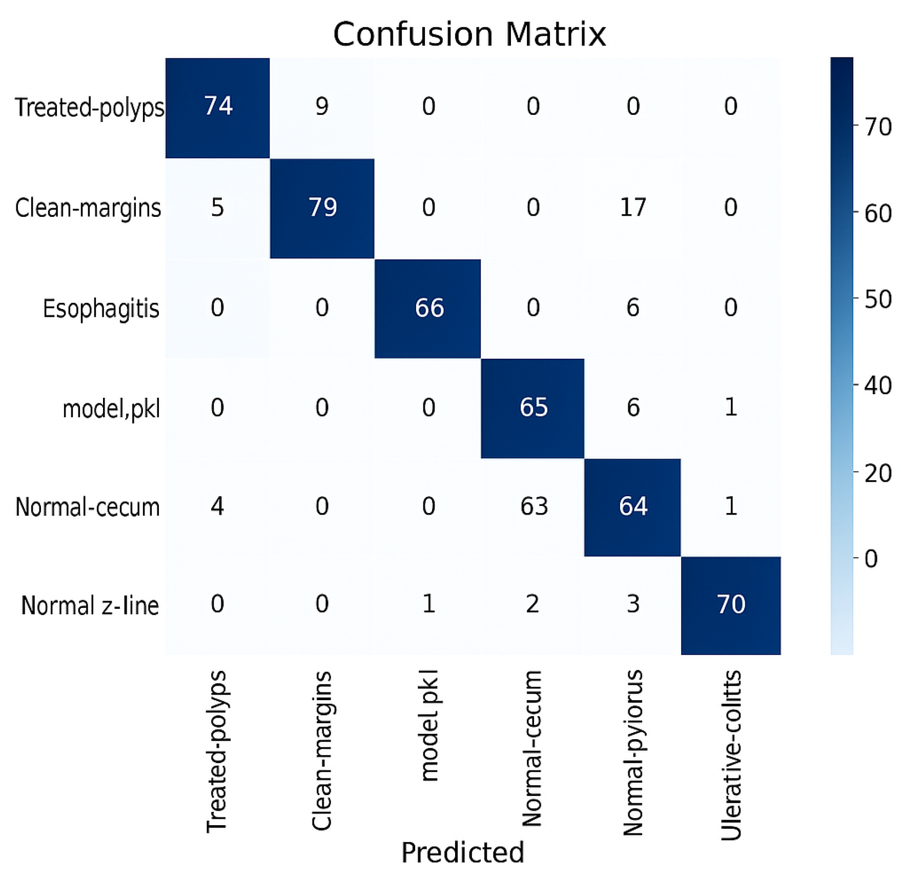
The right-side values are most likely the color bars; they define the range of values used in the heatmap shading. Each cell in the confusion matrix represents the count of predictions (e.g., the number of samples from class A that were incorrectly predicted as class B). The heatmap uses colors to visualize those counts. The values on the right -20,0,...,70 correspond to color intensity, not the actual data. The negative value (-20) likely suggests either an artifact in normalization, scaling, or it’s a misconfigured threshold, since confusion matrices usually don’t include negative values. As can be observed, the model that performed the best in this analysis, ResNet50, demonstrates confusion between visually similar classes while reaching high classification rates for some of them. Overlapping textures or color profiles, especially between polyps and inflamed mucosa, may be the cause of these misclassifications. On the other hand, visually recognized and well-represented classifications like normal or ulcerative-colitis consistently shown good precision and recall ratings.
4. Discussion
4.1. Improvements
To improve CNN model performance on gastrointestinal polyp classification from endoscopic images, the study implemented several targeted:
- Customised Data Augmentation: While augmentation is a standard technique, this study applies a task-specific augmentation pipeline, including rotation, scaling, flipping, and contrast adjustment—optimised for gastrointestinal polyp morphology. This approach reduces overfitting.
- Dynamic Class: A novel weighting scheme was implemented based on real-time class distribution during training, rather than static frequency-based weights. This improves learning stability across imbalanced classes.
- Explainability: Grad-CAM was integrated as a feedback mechanism during model refinement. This dual use helped identify misclassified regions and guided architectural adjustments [51].
While VGG16, SqueezeNet, and NASNetLarge showed promising learning rates early in training, extensive augmentation and architectural regularisation were critical to overcoming their overfitting behavior.
4.2. Error Analysis
Errors during CNN training were classified into two major types:
- Confusions between visually similar classes: The most frequent misclassifications involved visually similar classes, such as polyps and inflamed mucosa, which shared overlapping color gradients, mucosal textures, and ill-defined boundaries.
- Class Imbalance Sensitivity: These include inter-class confusion (e.g., misidentifying hyperplastic polyps as adenomatous ones) and incorrect localisation or attention to irrelevant image regions. Precision and recall were lower for classes with fewer representative samples, such as uncommon polyp subtypes. This results from bias caused during training.
These classification challenges were compounded by limitations in dataset diversity, inconsistent lighting, and the absence of pixel-level annotations. Solutions may include using advanced sampling strategies, synthetic data generation, or incorporating spatial attention mechanisms to focus learning on relevant image regions.
4.3. Limitations
Despite rigorous experimentation, the study encountered several constraints:
- Dataset Size: The Ksavir dataset contains a relatively limited number of images for certain polyp subtypes, which can impair generalisation and lead to classifier bias.
- Overfitting in Complex Models: Architectures like EfficientNetB8, InceptionResNetV2 and NASNetLarge demonstrated high variance between training and validation metrics, indicating overfitting. These models were excluded from the final evaluation.
- Domain Limitation: The trained models performed well on Ksavir data, but may experience performance degradation when applied to endoscopic images from different institutions, due to lighting conditions, device variability, and annotation inconsistency.
- Hardware Constraints: Training and tuning were conducted on an RTX 3050 GPU (4GB), which limited the ability to perform extensive hyperparameter tuning or ensemble testing across large architectures.
4.4. Proposals for future work (integration with segmentation, multi-label classification).
This work focused exclusively on image classification, but the following directions for future development could be considered:
- Integration of a segmentation component: where the model not only classifies but also highlights the affected area in the image. This could be achieved by U-Net or Mask R-CNN type models, which would add a significant plus to the system.
- Multi-label classification: multiple features or lesion types may appear in some images, so future models should be trained to recognize multiple classes simultaneously in a single image.
- Creation of a graphical user interface (GUI): allowing the clinician to load an image and get instant prediction, with the option to visualize the probability of each class.
- Model Explainability (XAI): to increase the confidence of physicians, techniques such as Grad-CAM could be integrated to visually show which region in the image was the basis for the network decision.
- Use of Vision Transformer (ViT) models: future work could investigate the replacement of CNNs with ViTs, attention-based models that provide competitive results in medical imaging, especially in fine lesion detection [52].
- Deployment of generative models (GANs): GANs can be used to generate synthetic medical images, increasing training sets and improving model generalization, especially in sparse or imbalanced classes [53].
- Implementation of MLOps solutions for clinical deployment: future research should include the development of automated pipelines for the integration of models into a real medical system, with monitored and updateable versions.
- Multimodal applications: future research may include models that combine medical images with clinical textual or demographic data, increasing decision context and accuracy.
Future studies might research cross-hospital training using federated learning, semi-supervised learning to integrate unlabeled data, and diagnostic integration through explainable AI interfaces customized based on physician input.
5. Conclusions
In this study, a biomimetic DL-based image classification model was developed to automatically identify GI lesions from endoscopic images using CNNs.
There were compared several deep learning models for automatic classification of gastrointestinal polyps in endoscopic images. It was performed with the aim to identify the architecture that provides the best results in accuracy and generalization ability. Actual state-of-the-art CNN models such as ResNet50 [18], DenseNet121 [31], MobileNetV2 [32] were used for training. Moreover, other architectures were also tested, some returned worse results due to overfitting.
Results show that the ResNet50 model obtained the best accuracy on the validation set, followed by MobileNetV2 and DenseNet121. The models were evaluated by accuracy and confusion matrix, their performances were compared in the previous chapter.
In order to assist users such as physicians, in Figure 6, an interface was also designed that allows the selection of one of the trained models mentioned above. The interface allows the user to select an image they wish to assign to a class and visualize which class the image belongs to, based on the previously selected model.
Even though the training time was significant (between 2 and 4 hours for each model), some stable results were obtained, and the differences between the accuracy on the training and validation set were small for the well-optimized models, indicating good generalization.
In practice, the models performed well even on consumer-grade hardware, being tested on a Lenovo IdeaPad Gaming 3 laptop (RTX 3050, i5-12500H). The average inference time for an image was under one second, allowing these systems to be integrated into a real-time workflow without significant differences. It was observed that most classifications were correct, especially for classes well represented in the training data. Classes with large variations or few examples were harder to classify, indicating the need for additional data.
In conclusion, this research presents an efficient biomimetic AI-based pipeline for medical image classification, demonstrating strong potential for aiding colorectal cancer screening and improving diagnostic in clinical environments.
6. Testing the ResNet50 Model Using a Graphical User Interface (GUI)
Trained models could be a tool for gastroenterologists, especially in endoscopic diagnostic procedures. A rapid classification of polyps could make early detection of precancerous lesions easier, thereby reducing the risk of colorectal cancer.
Figure 5a shows the graphical user interface that has been built to help users such as physicians to test the model. The interface allows the user to select one of the trained models for predictions. For predictions, the Load Image button needs to be clicked to select the image to be classified. Pressing the Start Classification button returns the class of the loaded image, using the model chosen by the user. The chosen model (ResNet50) was successful in predicting the image’s class in Figure 5b. According to the model, the image represents a polyp that belongs to the ulcer class, as predicted by the model.
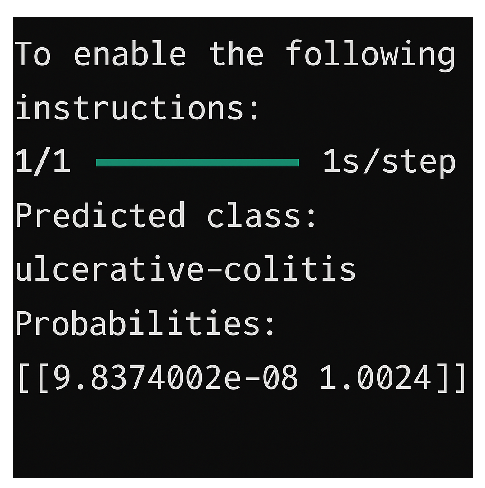
The selection of the trained models is an advantage for the clinician, as they can make a comparison for returning an accurate prediction. The result of a classification can be seen in Figure 6. The model loads an image, processes an image, and generates the model prediction in a very short time (1s/step), displaying the estimated class as shown in Figure 6, thus highlighting the practical applicability.
Figure 6.
Image-based inference.
Author Contributions
Conceptualization, C.-D.M; methodology, C.-D.M, I.-L.B.; software, C.-D.M; validation, C.-D.M. and N.-O.D.; formal analysis, C.-D.M. and N.-O.D.; investigation, C.-D.M., N.-O.D.; resources, C.-D.M; data curation, C.-D.M; writing—original draft preparation, C.-D.M., N.-O.D.; writing—review and editing, C.-D.M and I.-L.B.; visualization, C.-D.M.; supervision, I.-L.B.; project administration, C.-D.M. and N.-O.D.; funding acquisition, C.-D.M. and N.-O.D. All authors have read and agreed to the published version of the manuscript.
Funding
This research received no external funding.
Institutional Review Board Statement
Not applicable.
Data Availability Statement
The dataset consists of Simula Research Laboratory, Kvasir Dataset,
Acknowledgments
This research received financial support from ’1 Decembrie 1918’ University of Alba Iulia, Romania, through Order no. 3259 of 13th February 2025. The authors thank the Research Group on Artificial Intelligence and Data Science for Healthcare Innovation (REFLECTION) and the Research Center on Artificial Intelligence, Data Science, and Smart Engineering (ARTEMIS), of the George Emil Palade University of Medicine, Pharmacy, Science and Technology of Targu Mureş, Romania, for support of research infrastructure. The CA22137 COST Action, the Randomized Optimization Algorithms Research Network (ROAR-NET), with concerns in identifying benchmarking issues.
Conflicts of Interest
The authors declare no conflicts of interest.
References
- Ichihara, M.; et al. Long noncoding RNA 01534 maintains cancer stemness by downregulating endoplasmic reticulum stress response in colorectal cancer. Annals of Gastroenterological Surgery 2023, 7, 458–470. [CrossRef]
- Chitca, D.D.; et al. Advancing Colorectal Cancer Diagnostics from Barium Enema to AI-Assisted Colonoscopy. Diagnostics 2025, 15. [CrossRef]
- Puzzo, M.; et al. Colorectal Cancer: Current and Future Therapeutic Approaches and Related Technologies Addressing Multidrug Strategies Against Multiple Level Resistance Mechanisms. International Journal of Molecular Sciences 2025, 26. [CrossRef]
- Waldum, H.; Fossmark, R. Gastritis, Gastric Polyps and Gastric Cancer. International Journal of Molecular Sciences 2021, 22, 6548. [CrossRef]
- Siegel RL, Giaquinto AN, J. Global Cancer Statistics. CA: A Cancer Journal for Clinicians 2024, 74(2):203. [CrossRef]
- Cincar, K.; Sima, I. Machine Learning algorithms approach for Gastrointestinal Polyps classification. In Proceedings of the International Conference on INnovations in Intelligent SysTems and Applications, INISTA 2020, Novi Sad, Serbia, August 24-26, 2020. IEEE, 2020, pp. 1–6. [CrossRef]
- Lundberg, S.M.; Lee, S.I. A Unified Approach to Interpretable Machine Learning. Advances in Neural Information Processing Systems 2017, 30.
- Bishop, C.M. Pattern Recognition and Machine Learning; Information Science and Statistics, Springer: New York, NY, 2006.
- LeCun, Y.; Bengio, Y.; Hinton, G. Deep learning. Nature 2015, 521, 436–444. [CrossRef]
- Dong, Y.; Li, J.; Wang, Z.; Jia, W. CoDC: Accurate Learning with Noisy Labels via Disagreement and Consistency. Biomimetics 2024, 9, 92. [CrossRef]
- Wang, S.; Chen, H.; Zhang, Y. Bionic Artificial Neural Networks in Medical Image Analysis. Biomimetics 2023, 8, 211. [CrossRef]
- Consortium, M. A map of neural signals and circuits traces the logic of brain computation. Nature 2025. [CrossRef]
- Mienye, I.D.; et al. Deep Convolutional Neural Networks in Medical Image Analysis: A Review. Information 2025, 16. [CrossRef]
- Kountchev, R.; Iantovics, B.; Kountcheva, R. Hierarchical Third-Order Tensor Decomposition through Inverse Difference Pyramid, Based on the 3D Walsh-Hadamard Transform with Applications in Data Mining. WIREs Data Mining and Knowledge Discovery 2020, 10. [CrossRef]
- Krizhevsky, A.; Sutskever, I.; Hinton, G. ImageNet Classification with Deep Convolutional Neural Networks. Neural Information Processing Systems 2012, 25. [CrossRef]
- Simonyan, K.; Zisserman, A. Very Deep Convolutional Networks for Large-Scale Image Recognition. In Proceedings of the 3rd International Conference on Learning Representations (ICLR), 2015, pp. 1–14.
- Szegedy, C.; et al. Going Deeper with Convolutions. CVPR 2015, pp. 1–9. [CrossRef]
- He, K.; et al. Deep Residual Learning for Image Recognition. In Proceedings of the Proceedings of the IEEE Conference on Computer Vision and Pattern Recognition (CVPR), 2016, pp. 770–778.
- Huang, G.; Liu, Z.; Van Der Maaten, L.; Weinberger, K.Q. Densely Connected Convolutional Networks. Proceedings of the IEEE Conference on Computer Vision and Pattern Recognition 2017, pp. 4700–4708.
- Gong, E.J.; Bang, C.S.; Lee, J.J. Edge Artificial Intelligence Device in Real-Time Endoscopy for Classification of Gastric Neoplasms: Development and Validation Study. Biomimetics 2024, 9. [CrossRef]
- Nazir, A.; et al. A deep learning-based novel hybrid CNN-LSTM architecture for efficient detection of threats in the IoT ecosystem. Ain Shams Engineering Journal 2024, 15. [CrossRef]
- Zhen, L.; Bărbulescu, A. Comparative Analysis of Convolutional Neural Network-Long Short-Term Memory, Sparrow Search Algorithm-Backpropagation Neural Network, and Particle Swarm Optimization-Extreme Learning Machine Models for the Water Discharge of the Buzău River, Romania. Water 2024, 16. [CrossRef]
- Jalan, A.; Mishra, D.; Marisha.; Gupta, M. Diagnosis of Schizophrenia Using Feature Extraction from EEG Signals Based on Markov Transition Fields and Deep Learning. Biomimetics 2025, 10, 449. [CrossRef]
- Iman, M.; Arabnia, H.R.; Rasheed, K. A Review of Deep Transfer Learning and Recent Advancements. Technologies 2023, 11, 40.
- Mallouk, O.; Joudar, N.E.; Ettaouil, M. A Selective Model for Transfer Learning in CNNs: Optimization of Fine-Tuning Layers. International Journal of Data Science and Analytics 2024.
- Selvaraju, R.R.; Cogswell, M.; Das, A.; Vedantam, R.; Parikh, D.; Batra, D. Grad-CAM: Visual Explanations from Deep Networks via Gradient-Based Localization. Proceedings of the IEEE International Conference on Computer Vision 2017, pp. 618–626.
- Pogorelov, K.; et al. Kvasir: A Multi-Class Image-Dataset for Computer Aided Gastrointestinal Disease Detection, 2017. [CrossRef]
- Muratarat, M. Kvasir Dataset v2 Classifier. https://github.com/mmuratarat/kvasir-v2-ViT-classifier, 2024. GitHub Repository.
- Demirbaş, A.A.; Üzen, H.; Fırat, H. Spatial-attention ConvMixer architecture for classification and detection of gastrointestinal diseases using the Kvasir dataset. Health Information Science and Systems 2024, 12, 32.
- Demirbaş, A.A.; Üzen, H.; Fırat, H. Automated classification of gastrointestinal diseases using deep learning. Medical & Biological Engineering & Computing 2024, 63, 293–320. [CrossRef]
- Huang, G.; Liu, Z.; Van Der Maaten, L.; Weinberger, K.Q. Densely Connected Convolutional Networks. In Proceedings of the Proceedings of the IEEE Conference on Computer Vision and Pattern Recognition (CVPR), 2017, pp. 4700–4708.
- Sandler, M.; et al. MobileNetV2: Inverted Residuals and Linear Bottlenecks. In Proceedings of the Proceedings of the IEEE Conference on Computer Vision and Pattern Recognition (CVPR), 2018, pp. 4510–4520.
- Szegedy, C.; et al. Rethinking the Inception Architecture for Computer Vision. In Proceedings of the Proceedings of the IEEE Conference on Computer Vision and Pattern Recognition (CVPR), 2016, pp. 2818–2826.
- Chollet, F. Xception: Deep Learning with Depthwise Separable Convolutions. In Proceedings of the Proceedings of the IEEE Conference on Computer Vision and Pattern Recognition (CVPR), 2017, pp. 1251–1258.
- Simonyan, K.; Zisserman, A. Very Deep Convolutional Networks for Large-Scale Image Recognition. In Proceedings of the International Conference on Learning Representations (ICLR), 2015.
- Iandola, F.N.; et al. SqueezeNet: AlexNet-level accuracy with 50x fewer parameters and <0.5MB model size. arXiv preprint arXiv:1602.07360, 2016.
- Howard, J.; Gugger, S. xResNet architectures within FastAI. https://docs.fast.ai/vision.models.xresnet.html, 2020.
- He, K.; et al. Deep Residual Learning for Image Recognition. In Proceedings of the Proceedings of the IEEE Conference on Computer Vision and Pattern Recognition (CVPR), 2016, pp. 770–778.
- Esmaeilzadeh, H.; Ghodrati, S.; Kahng, A.B. Performance Analysis of DNN Inference/Training with Convolution and Non-Convolution Operations. arXiv 2023.
- Sandler, M.; Howard, A.; Zhu, M.; Zhmoginov, A.; Chen, L. MobileNetV2: Inverted Residuals and Linear Bottlenecks. Proceedings of the IEEE Conference on Computer Vision and Pattern Recognition 2018, pp. 4510–4520.
- Yang, X.; Zhang, W.; Li, J. Challenges in CNN-Based Medical Image Analysis and Future Directions. Journal of Medical AI Research 2024, 12, 45–62. [CrossRef]
- Zoph, B.; et al. Learning Transferable Architectures for Scalable Image Recognition. In Proceedings of the Proceedings of the IEEE Conference on Computer Vision and Pattern Recognition (CVPR), 2018, pp. 8697–8710.
- Tan, M.; Le, Q.V. EfficientNet: Rethinking Model Scaling for Convolutional Neural Networks. In Proceedings of the Proceedings of the International Conference on Machine Learning (ICML), 2019, pp. 6105–6114.
- Liu, Z.; et al. A ConvNet for the 2020s. IEEE/CVF Conference on Computer Vision and Pattern Recognition (CVPR) 2022, pp. 11976–11986.
- Szegedy, C.; Ioffe, S.; Vanhoucke, V.; Alemi, A. Inception-v4, Inception-ResNet and the Impact of Residual Connections on Learning. arXiv preprint 2017, [1602.07261].
- Huang, G.; et al. Densely Connected Convolutional Networks. In Proceedings of the Proceedings of the IEEE Conference on Computer Vision and Pattern Recognition (CVPR), 2017, pp. 4700–4708.
- Kaur, G.; Saini, S. Comparative Analysis of RMSE and MAP Metrics for Evaluating CNN and LSTM Models. AIP Conference Proceedings 2024, 3121, 040003.
- Zhukov, A.; Benois-Pineau, J.; Giot, R. Reference-based and No-reference Metrics to Evaluate Explanation Methods of AI - CNNs in Image Classification Tasks. arXiv 2024.
- Nazir, Z.; Yarovenko, V.; Park, J.G. Interpretable ML Enhanced CNN Performance Analysis of cuBLAS, cuDNN, and TensorRT. ResearchGate 2023.
- Düntsch, I.; Gediga, G. Confusion Matrices and Rough Set Data Analysis. In Proceedings of the Proceedings of the 2019 International Conference on Pattern Recognition and Intelligent Systems (PRIS). arXiv, 2019. [CrossRef]
- Team, T.R. Multiclass Confusion Matrix for Object Detection. Edge AI and Vision Alliance 2023.
- Dosovitskiy, A.; et al. An Image is Worth 16x16 Words: Transformers for Image Recognition at Scale. arXiv preprint arXiv:2010.11929 2020.
- Yi, X.; Walia, E.; Babyn, P. Generative Adversarial Network in Medical Imaging: A Review. Medical Image Analysis 2019, 58, 101552. [CrossRef]
Figure 1.
Summary of the proposed workflow for automatic classification of gastrointestinal lesions. The pipeline consists of four core stages: image acquisition, preprocessing, CNN-based model training and inference, and final evaluation using classification metrics and explainability tools.
Figure 1.
Summary of the proposed workflow for automatic classification of gastrointestinal lesions. The pipeline consists of four core stages: image acquisition, preprocessing, CNN-based model training and inference, and final evaluation using classification metrics and explainability tools.
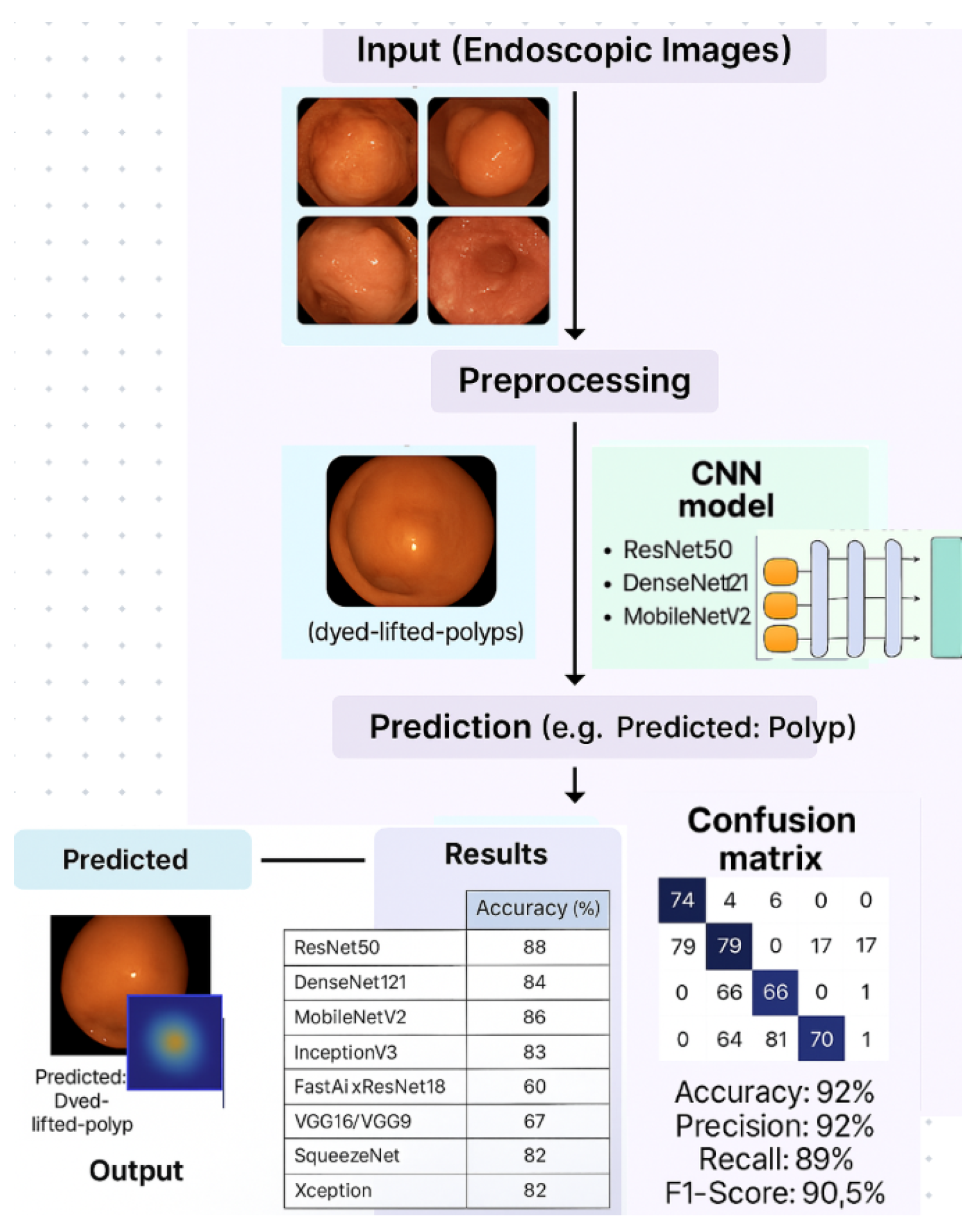
Figure 2.
Accuracy networks models. (a) ResNet50 Accuracy. (b) ResNet50 Loss. (c) DenseNet121 Accuracy. (d) MobileNetV2 Accuracy. (d) MobileNetV2 Loss. (d) FastAI Accuracy.
Figure 2.
Accuracy networks models. (a) ResNet50 Accuracy. (b) ResNet50 Loss. (c) DenseNet121 Accuracy. (d) MobileNetV2 Accuracy. (d) MobileNetV2 Loss. (d) FastAI Accuracy.
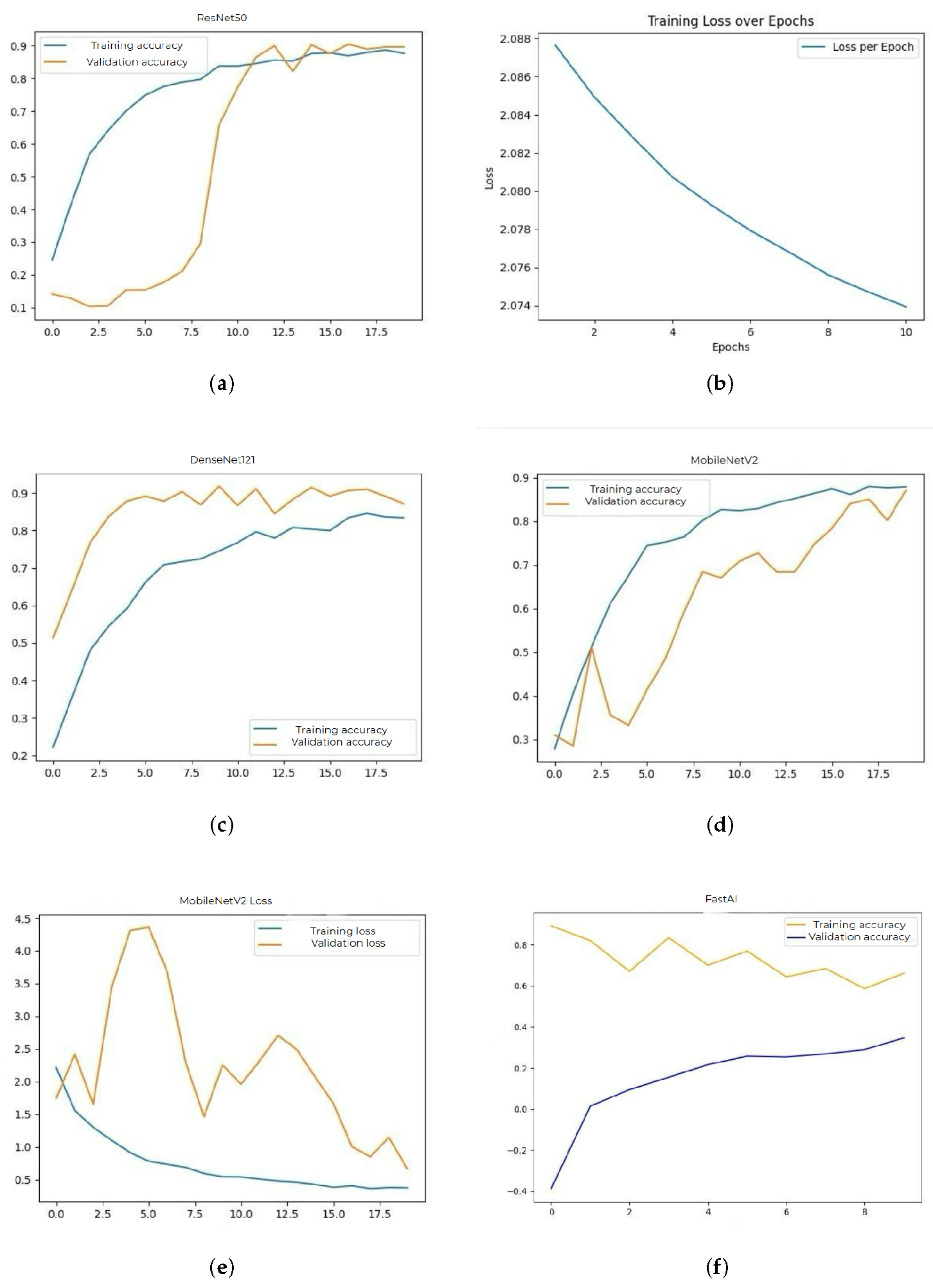
Figure 3.
Accuracy networks models (cont.). (a) InceptionV3 Accuracy. (b) InceptionV3 Loss. (c) VGG16 - VGG19 Accuracy. (d) SqueezeNet Accuracy. (d) Xception Accuracy. (d) Xception Loss.
Figure 3.
Accuracy networks models (cont.). (a) InceptionV3 Accuracy. (b) InceptionV3 Loss. (c) VGG16 - VGG19 Accuracy. (d) SqueezeNet Accuracy. (d) Xception Accuracy. (d) Xception Loss.
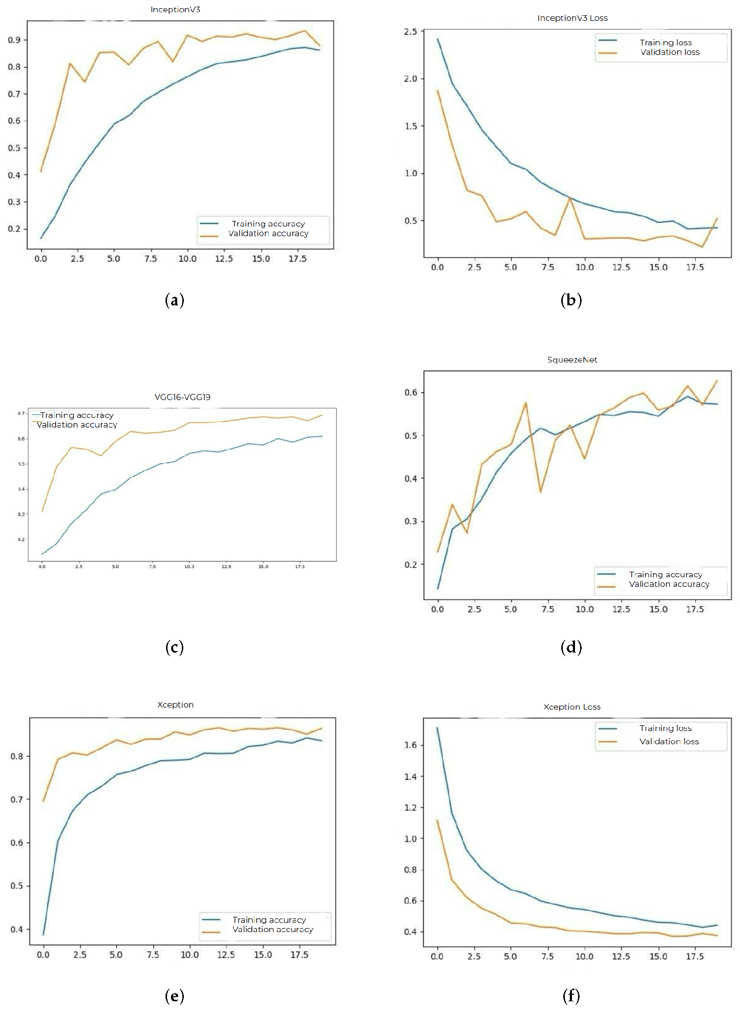
Figure 5.
Graphical interface evaluation and real-image testing. (a) Custom-built GUI for gastrointestinal polyp classification using the Xception model. The interface includes model selection, image input, and output prediction functionality, in this instance, displaying Predicted class: rectum. (b) Endoscopic image of a real gastrointestinal polyp used for testing and validating model prediction in real-world conditions.
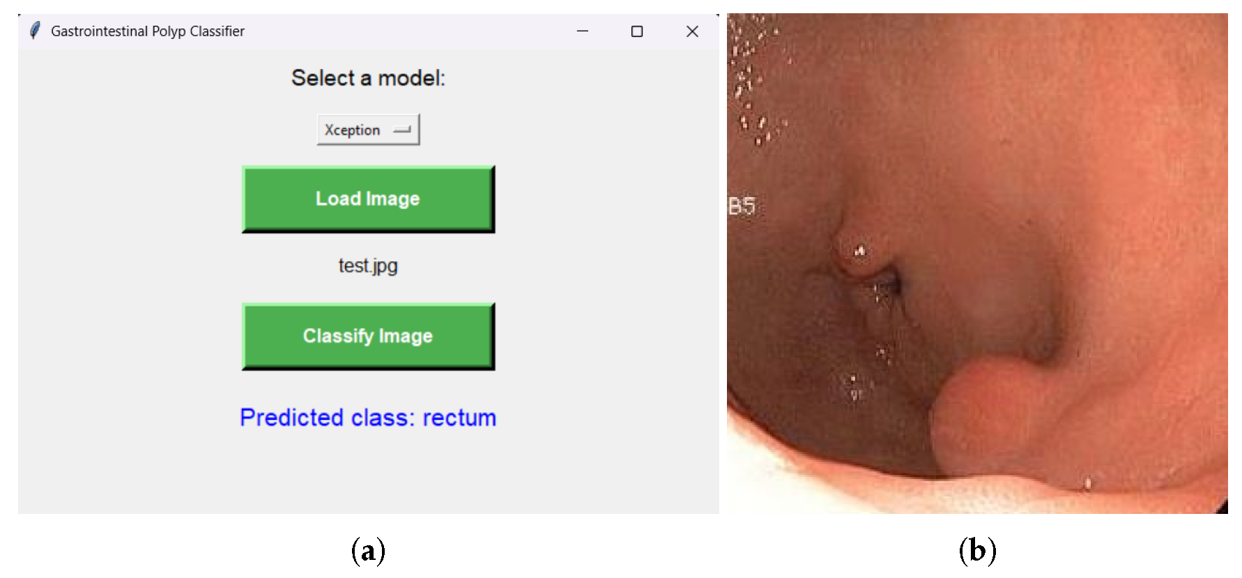

Table 1.
Performance comparison of CNN models on the Ksavir test set: Accuracy, Precision, Recall, and F1-score.
Table 1.
Performance comparison of CNN models on the Ksavir test set: Accuracy, Precision, Recall, and F1-score.
| Model | Train | Valid | Prec | Rec | F1 | Predicted Class |
|---|---|---|---|---|---|---|
| ResNet50 | 88% | 90% | 92% | 89% | 90.5% | dyed-lifted-polyps |
| DenseNet121 | 84% | 87% | 89% | 86% | 87.5% | dyed-resection-margins |
| MobileNetV2 | 86% | 87% | 88% | 85% | 86.5% | esophagitis |
| InceptionV3 | 83% | 85% | 86% | 83% | 84.5% | normal-cecum |
| FastAI xResNet18 | 64% | 70% | 74% | 68% | 71.0% | normal-pylorus |
| VGG16/VGG19 | 60% | 68% | 70% | 63% | 66.0% | normal-z-line |
| SqueezeNet | 57% | 63% | 68% | 59% | 63.0% | polyps |
| Xception | 82% | 85% | 85% | 84% | 84.5% | ulcerative-colitis |
Disclaimer/Publisher’s Note: The statements, opinions and data contained in all publications are solely those of the individual author(s) and contributor(s) and not of MDPI and/or the editor(s). MDPI and/or the editor(s) disclaim responsibility for any injury to people or property resulting from any ideas, methods, instructions or products referred to in the content. |
© 2025 by the authors. Licensee MDPI, Basel, Switzerland. This article is an open access article distributed under the terms and conditions of the Creative Commons Attribution (CC BY) license (http://creativecommons.org/licenses/by/4.0/).
Copyright: This open access article is published under a Creative Commons CC BY 4.0 license, which permit the free download, distribution, and reuse, provided that the author and preprint are cited in any reuse.


