
Submitted:
22 July 2025
Posted:
22 July 2025
You are already at the latest version
Abstract
This study presents a reconfigurable optical convolutional neural network (CNN) architecture that integrates a crossbar switch network into a smart-pixel-based optical CNN (SPOCNN) framework. The SPOCNN leverages smart pixel light modulators (SPLMs), enabling high-speed and massively parallel optical computation. To address the challenge of data rearrangement between CNN layers—especially in multi-channel and deep-layer processing—a crossbar switch network is introduced to perform dynamic spatial permutation and multicast operations efficiently. This integration significantly reduces the number of processing steps required for core operations such as convolution, max pooling, and local response normalization, enhancing throughput and scalability. The architecture also supports bidirectional data flow and modular expansion, allowing the simulation of deeper networks within limited hardware layers. Performance analysis based on an AlexNet-style CNN indicates that the proposed system can complete inference in fewer than 100 instruction cycles, achieving processing speeds of over 1 million frames per second. The proposed architecture offers a promising solution for real-time optical AI applications. Further development of hardware prototypes and co-optimization strategies between algorithms and optical hardware is suggested to fully harness its capabilities.
Keywords:
optical neural network
; convolution
; smart pixel
; crossbar switch
1. Introduction
In recent years, convolutional neural networks (CNNs) have achieved remarkable progress in various fields such as image recognition, audio processing, and natural language understanding, owing to their powerful pattern recognition capabilities and hierarchical feature extraction mechanisms [1,2]. CNNs operate by applying a series of convolutional kernels to input data, allowing the network to extract spatial and temporal features [3]. As the demand for more complex CNN architectures grows, challenges related to computational speed, scalability, and energy consumption have become increasingly significant, especially in real-time inference scenarios and edge computing environments.
Conventional electronic processors such as graphics processing units and tensor processing units (TPUs) have been widely used to accelerate CNN operations [4]. However, these electronic systems often face inherent limitations, including high power consumption [5], restricted memory bandwidth [6], and latency caused by data transfers and synchronization processes [7]. Additionally, scaling large CNN models across multiple processing units introduces significant interconnect bottlenecks, leading to further inefficiencies in real-time processing tasks [8]. Consequently, alternative computing architectures have been actively explored to address these challenges.
One promising alternative is optical computing, which leverages the inherent parallelism and high bandwidth of light to perform computations at the speed of light while significantly reducing power consumption. Traditional optical CNN implementations have primarily employed 4f correlator systems [9,10,11,12] that utilize Fourier optics to perform convolutions [13]. Despite their ability to execute parallel convolutions, 4f correlator-based systems face several drawbacks, including limited scalability imposed by the finite space-bandwidth product of optical components [9], geometric aberrations, and the slow refresh rates of spatial light modulators (SLMs) used for kernel pattern generation.
To overcome these limitations, previous studies have introduced scalable optical convolutional neural network (SOCNN) architectures based on free-space optics using lens arrays and spatial light modulators [14,15,16]. These architectures allow for scalable input sizes and direct kernel representation, mitigating some challenges of the 4f correlator systems. However, SLM-based systems still suffer from slow refresh rates, typically operating in the kilohertz range [17,18], which restricts their ability to support real-time weight updates and dynamic kernel reconfiguration.
Smart-pixel-based optical convolutional neural networks (SPOCNNs) have been proposed as a further advancement, replacing SLMs with smart pixel light modulators (SPLMs) that integrate photodetectors, electronic processors, and light-emitting diodes within each pixel [19,20,21]. The inclusion of electronic processors and memory within SPLMs enables rapid weight updates, reaching refresh rates in the hundreds of megahertz, while maintaining optical parallelism. SPOCNNs not only enhance reconfigurability and scalability but also simplify the optical design by reducing alignment complexities and eliminating the need for coherent light sources.
While SPOCNNs provide significant improvements, one remaining challenge lies in efficiently managing data rearrangement between convolutional layers, particularly when dealing with multi-page data formats such as color image channels or high-dimensional feature maps. The conventional SPOCNN architecture may require multiple sequential steps or complex spatial transformations to reorganize data for the subsequent convolutional layers, leading to additional latency and diminished parallel processing benefits.
To address this challenge, this study proposes a novel conceptual architecture that integrates a crossbar switching network into the smart-pixel-based optical CNN framework. The crossbar switch enables multicast and efficient spatial permutation of data between layers, allowing arbitrary reorganization of output data to align with the input format of subsequent convolutional layers. This integration significantly reduces the number of sequential processing steps required for data reorganization and enhances the overall parallel processing capability of the system.
By leveraging the high-speed reconfigurability of SPLMs and the flexible connectivity of crossbar switches, the proposed architecture offers a promising pathway toward highly scalable and efficient optical CNNs capable of handling complex multi-layer structures with minimal latency. The following sections will present a detailed conceptual design of the proposed system, analyze its operational principles, and discuss its potential advantages over existing architectures.
2. Materials and Methods
To explain the architecture of the SPOCNN incorporating crossbar switches, it is essential to first examine the structure and operation of a typical CNN. We aim to demonstrate how the SPOCNN, along with crossbar switches, can be employed to implement conventional CNN procedures. The general CNN architecture is illustrated in Figure 1, and the detailed layer specifications—including input, output, and kernel array sizes—are summarized in Table 1 [22]. This layer configuration closely resembles that of AlexNet.
Suppose that the SPOCNN architecture shown in Figure 2 is used to implement the layer structure described in Table 1. The first convolutional layer, Conv1, receives three input images (R, G, B), each with a resolution of 227 × 227, and produces 96 output feature maps of size 55 × 55 when using an 11 × 11 kernel with a stride of 4. One approach to performing convolution with SPOCNN is to process one image at a time, storing the outputs for all 96 filters. After processing the R image, the same procedure is applied to the G and B images. This results in a total of 96 × 3 sequential steps for the Conv1 layer.
The number of operations per step is (227 × 227) × (11 × 11), requiring a minimum SPLM array size of 2,497 × 2,497 to process the entire input image without fragmentation. If such a large SPLM array is unavailable, the input must be divided into smaller patches and recombined, as described in the transverse scaling method using SPLM memory [21], which increases the number of steps and introduces processing delays.
Although this method leverages the optical parallelism of SPOCNN, it does not fully exploit its potential. One of SPOCNN’s key advantages is its ability to handle arbitrarily large input and output arrays. However, the method above limits the input size to 227 × 227. This limitation becomes more pronounced in subsequent layers, such as Conv2. The Conv2 layer receives input of size 27 × 27 × 96 and produces output of size 27 × 27 × 256 using 5 × 5 kernels. In this case, the required SPLM array size is only 135 × 135—significantly smaller than the 2,497 × 2,497 needed for Conv1.
If an SPLM array of 2,497 × 2,497 is allocated for Conv1, most of the array would remain idle during Conv2. To improve resource utilization and parallel throughput, feature maps from the 27 × 27 input array can be duplicated and tiled into a larger 2,497 × 2,497 array. For example, 96 feature maps can be arranged in a 12 × 8 macro-array, where each sub-array is 27 × 27. This results in a composite array of size 324 × 216 pixels, requiring a 1,620 × 1,080 SPLM array when accounting for the 5 × 5 kernel size. Tiling in this way significantly improves SPLM utilization and throughput.
However, transferring data from the original 27 × 27 input to the 324 × 216 tiled output is feasible but inefficient in SPOCNN. As shown in Figure 2, the maximum data transfer range is limited by half the kernel size. If the maximum kernel size is 11, the step size is only 5, requiring 30 sequential moves to shift the data to the farthest tile. Moreover, data replication and movement are not inherently parallel operations and demand additional algorithmic complexity. This issue of data rearrangement commonly arises between layers—especially when the data format changes substantially.
indicates the i-th neural network node in the j-th layer [21].
To address the issue of data rearrangement between layers, we introduce a crossbar switch network positioned either between convolutional layers or directly after the output nodes, as illustrated in Figure 3(a). The crossbar switch is a well-established component in communication and computer network systems, and it exists in both electronic and optical forms [23,24,25,26]. When a switch is turned ON, the corresponding horizontal line connects electrically to the vertical line at the crossing point. Since the crossbar switch forms a two-dimensional matrix, each crossing point can be individually turned ON or OFF, with its state programmable through data stored in memory.
For example, if the output node is connected to a horizontal wire and the crossbar switch at position (i, j) is ON, then is routed to . If multiple switches in a row are ON while others remain OFF, the input signal is sent to multiple outputs simultaneously—this is referred to as multicast [24,25,26]. If only one switch in a row is ON, the signal is routed to a single output—this is called unicast. When multiple switches in the same column are ON, it results in contention or an output conflict, which is typically undesirable and requires scheduling or arbitration mechanisms.
In cases where the output is treated as current, simultaneous activation of multiple switches in a column may be interpreted as a summation operation. However, this current-based addition is excluded from consideration for now. Such scenarios are better managed using merge connections, where inputs are sequentially linked to a shared output via unicast operations. Although this approach introduces delays due to serialization, merge operations can still be useful for implementing certain algorithms.
A particularly valuable case is when N input lines are connected to N output lines via unicast connections exclusively. In this configuration, the crossbar switch effectively performs a permutation, enabling arbitrary rearrangement of input data at the output. This is highly beneficial for reformatting data between layers in the SPOCNN architecture.
The physical layout of the SPOCNN integrated with a crossbar switch network is shown in Figure 3(b), and a 3D view of the configuration is presented in Figure 3(c). The 3D schematic illustrates how horizontal and vertical crossbar switch planes interconnect to support the rearrangement of two-dimensional arrays of neural network nodes. Each horizontal plane receives inputs from a row of output nodes in the previous layer and reorganizes the data sequence, while each vertical plane performs vertical rearrangement.
Buffers or bypass circuits can be placed between these planes or at their endpoints to store intermediate data. These buffers can also enable reverse data transmission to the input nodes, leveraging the bidirectional nature of the crossbar switch. This is particularly useful for bidirectional SPOCNN architectures, such as the two-mirror-like SPOCNN [21], where data flows back and forth between two physical layers. This design allows the emulation of an arbitrary number of virtual layers using only two physical hardware layers.
An advanced configuration that leverages the bidirectional nature of both the SPOCNN and the crossbar switch network is illustrated in Figure 4. To control data flow between layers, additional switches are incorporated both after the preceding layer and before the subsequent one. When the rearranged data stored in the output buffer of the crossbar switch is routed backward to the neural network nodes, these switches determine whether the data flows to the previous or the next layer.
Specifically, if Switch 1 is ON and Switch 2 is OFF, the data flows to the previous layer; conversely, if Switch 1 is OFF and Switch 2 is ON, the data proceeds to the next layer. Additionally, when all crossbar switches are OFF, the network functions in bypass mode. As a result, the crossbar switch network in Figure 4 effectively operates as a three-way switch. In the 3D configuration, the outputs of the next layer are connected to the horizontal crossbar switch plane through the bypass output channels.
Another advantage of the switch configuration shown in Figure 4 is that it can be placed between layers in a cascading manner along a straight path, without requiring a 90-degree change in direction. The multilayer SPOCNN architecture incorporating crossbar switches is illustrated in Figure 5. This configuration serves as a fundamental building block that can be repeated to form multiple physical layers to enhance parallelism, although it can also simulate additional layers by allowing data to flow back and forth within the same module.
In this architecture, the first layer , consisting of photodetectors and electronic processors (EPs), receives input data in real time from an optical imaging device and sends its output to the first crossbar switch (crossbar1). Crossbar1 rearranges the data and routes it to the second layer . The second and third layers perform optical convolution and other operations with dense interconnections. The resulting output is then passed through the second crossbar switch (crossbar2), which reorganizes the data and routes it to . At this stage, effectively becomes , now using updated weights stored in memory.
Layer executes another convolution or function in the reverse direction, and the resulting output is stored on the opposite side—originally , now serving as . In this manner, the SPOCNN architecture combined with crossbar switches can emulate a deep multilayer neural network, enabling flexible data flow and repeated processing within a compact physical system.
In Figure 5, the core optical component is the SPOCNN architecture; however, it can be substituted with other types of optical neural network structures, such as SPLM-based bidirectional optical neural network (SPBONN) [27,28], which features fully connected layers rather than partially connected ones. Multiple modules incorporating different optical cores can be cascaded to form a more efficient system, capable of handling varying data sizes or performing diverse functions.
3. Results
An investigation of the layer architecture, as shown in Table 1, reveals that the CNN primarily consists of convolution, max pooling, and local response normalization (LRN) operations applied to feature maps of varying sizes. Consequently, understanding how these operations can be implemented within the SPOCNN environment using crossbar switches is essential for evaluating the efficiency of the proposed architecture.
Figure 6 illustrates how convolution is applied to feature maps in this system. This form of convolution differs from the standard 2D convolution typically performed by SPOCNN [21]. While SPOCNN generally processes two-dimensional data arrays, convolution on feature maps involves depth, with both the data and kernel represented as three-dimensional arrays. In this case, convolution must be applied to each feature map independently, and the results at corresponding spatial coordinates must be summed across the entire depth.
In the example shown in Figure 6, the input consists of 16 feature maps, each of size 4 × 4. These feature maps are duplicated and tiled into a 4 × 4 macro-array using the multicast function of the crossbar switch, as depicted in the second step. A 3 × 3 kernel is then applied to each feature map, reducing each to a 2 × 2 array while preserving the 4 × 4 macro-array structure. The crossbar switch then uses its permutation capability to reorganize the convolution outputs into four colored sections, where each section aggregates results from different feature maps corresponding to a specific output coordinate.
In the final step, data within each color group is summed by a convolution operation—effectively performing a summation across the depth of the feature maps. Without this tiling and reorganization, convolution would need to be performed separately for each feature map, followed by 16 summations (equal to the number of feature maps). The conventional approach would require a total of 32 steps. In contrast, the proposed method completes the same process in just four steps, assuming the input data is pre-arranged into a tiled macro-array, as provided by the preceding layer in this architecture. Furthermore, in the proposed architecture, the number of processing steps remains constant regardless of the number of feature maps, whereas the conventional method scales linearly with depth.
The max pooling operation on feature maps using the SPOCNN with a crossbar switch is illustrated in Figure 7. In this example, the pooling window size is 3 × 3, and the stride is 2. As a result, the output appears every two pixels, with the gray pixels in Figure 7 representing the resulting pooled values.
The sequence of operations is indicated by arrows of different colors. In each step, data is moved and the max function is applied between the incoming pixel value and the current target pixel. The numbers in parentheses indicate the sets of data involved in the max operations performed up to that point. After four steps, all values within the 3 × 3 window are compared to determine the maximum output.
This process is highly parallelizable. When applied to a tiled feature map, the total number of steps remains constant at four, regardless of the input array size.
The LRN operation using the SPOCNN with a crossbar switch is illustrated in Figure 8. Like depth-wise convolution, LRN is also performed across feature maps. In the example shown in Figure 8, the normalization window size is 3.
When feature maps are tiled in a two-dimensional macro-array, the LRN operation requires accessing pixelwise data from both the preceding and succeeding feature maps. This is achieved by shifting each pixel’s data one map forward and one map backward within the macro-array, requiring only two steps. This movement is made possible through the permutation functionality of the crossbar switch.
If the normalization window size increases to 5, the number of required steps also increases accordingly to four. In this way, LRN operations can be efficiently performed with high parallelism using the SPOCNN architecture combined with crossbar switching.
4. Discussion
In the previous sections, we described the functions of the crossbar switch and the methods for applying it within the SPOCNN architecture to implement the three core layer operations: convolution, max pooling, and LRN. We now analyze how many steps or instruction cycles are required to complete the full layer architecture, as summarized in Table 1. The analysis assumes a hardware configuration based on the schematic in Figure 5.
The program begins with the first layer, which receives data in real time from an optical imaging device. The data acquired by the detector array in the first layer is processed through electronic processors and routed to the first crossbar switch (crossbar1). Each node in the first layer stores RGB image data with a resolution of 227 × 227. The three color channels are multicast to form a 227 × 681 array. This array is processed simultaneously as a regional block in the convolution layer, as illustrated in Figure 6. The process illustrated in Figure 6 corresponds to applying a single kernel across all feature maps.
To further increase parallel throughput, multiple kernel blocks are tiled within the convolution layer. For instance, if 96 blocks (arranged in a 12 × 8 grid) are tiled in the second layer, the entire dataset can be processed simultaneously. Accommodating these tiled maps in two dimensions requires an SPLM array of 29,964 × 59,928. Although this size is extremely large, we assume its feasibility, as the SPOCNN framework does not impose a theoretical limit on array size. Multicasting the three color maps to 96 kernel sets takes six instruction cycles—two for each color channel.
Once the tiled maps are ready, Conv1 is executed with an 11 × 11 kernel and a stride of 4, yielding a 55 × 55 × 96 output array. This convolution layer requires three instruction cycles, as shown in Figure 6. The LRN1 layer performs normalization with a window size of 5, requiring four steps and five instruction cycles—the additional cycle accounts for final computations using accumulated data. The Pool1 layer performs max pooling using a 3 × 3 window and a stride of 2, following a process similar to that shown in Figure 4. This step requires four iterations and eight instruction cycles, as each step involves both data shifting and a max operation. Rearranging the data format after Pool1 requires a multicast operation, which takes two additional instruction cycles.
Similarly, Conv2, LRN2, and Pool2 follow the same procedures and together require a total of 16 instruction cycles. Conv3, Conv4, and Conv5 collectively require 12 instruction cycles, as feature maps with depths exceeding 11 × 11 require an additional cycle to perform the final summation. Pool5 requires eight instruction cycles. Including four intermediate data rearrangement operations adds another eight instruction cycles.
Following the convolutional layers, three fully connected layers are executed. If the output nodes from Figure 5 are connected to another module—identical in structure but incorporating an SPBONN [28] core that performs full connectivity—with an input/output array of 128 × 128, then the FC6, FC7, and FC8 layers can be completed in just three steps, without requiring any data rearrangement.
In total, completing the CNN described in Table 1 requires approximately 71 instruction cycles. While this is a rough estimate, the total is expected to remain under 100 cycles. Assuming each instruction cycle takes approximately 10 ns, the processing time for a single image frame is about 1 µs, corresponding to a throughput of 1 million frames per second. Further system optimization and reduction of instruction cycle duration could result in even higher throughput. The analysis of instruction cycles is summarized in Table 2.
5. Conclusions
This study introduces a reconfigurable optical convolutional neural network (CNN) architecture—SPOCNN—enhanced by a crossbar switch network. The SPOCNN utilizes SPLMs that integrate light sources, photodetectors, and electronic processors within each pixel. This integration allows rapid weight updates and high-speed optical computation. While SPOCNN already improves upon traditional optical CNNs by enabling greater scalability and speed, its data rearrangement between layers remains a challenge—especially for multi-channel inputs and deep-layer architectures.
To overcome this limitation, a novel integration of crossbar switches is proposed. Crossbar switches enable efficient, programmable spatial permutation and multicast of data across neural layers, significantly reducing the number of sequential operations required for data reformatting. The study explores how core CNN operations—convolution, max pooling, and LRN—can be implemented in this architecture with high parallelism. Specific examples show that complex feature map operations traditionally requiring dozens of steps can now be completed in as few as four steps using the crossbar-enhanced SPOCNN.
The architecture also supports bidirectional data flow and modular stacking, enabling the simulation of deeper networks using fewer physical layers. This reconfigurable structure can accommodate various optical cores, including fully connected optical networks such as SPBONNs, and can efficiently handle diverse data formats and operations.
Simulation of an AlexNet-style CNN indicates that the entire network can be executed in approximately 71 instruction cycles—potentially under 100 in worst-case scenarios—with each cycle lasting around 10 ns. This results in an estimated processing speed of 1 million frames per second.
In conclusion, the integration of a crossbar switch network into the SPOCNN framework provides a compelling solution to the longstanding challenge of data reorganization in optical CNNs. This enhancement enables high-throughput, scalable, and reconfigurable deep neural network computation in the optical domain. By efficiently implementing convolution, pooling, and normalization operations—and leveraging the programmable, bidirectional capabilities of crossbar switches—the proposed architecture offers a promising pathway toward real-time, low-latency optical AI systems capable of processing frame rates exceeding 1 million frames per second. Future work involving hardware prototyping and algorithm–hardware co-optimization will be essential to fully realize the potential of this approach.
Funding
This research received no external funding
Data Availability Statement
The datasets generated during and/or analyzed during the current study are available from the corresponding author on reasonable request.
Acknowledgments
In this section, you can acknowledge any support given which is not covered by the author contribution or funding sections. This may include administrative and technical support, or donations in kind (e.g., materials used for experiments).
Conflicts of Interest
The authors declare no conflicts of interest.
Abbreviations
The following abbreviations are used in this manuscript:
| CNN | Convolutional neural network |
| EP | Electronic processor |
| LD | Laser diode |
| LED | Light-emitting diode |
| LRN | Local response normalization |
| OCNN | Optical convolutional neural network |
| PD | Photo detector |
| SPBONN | Smart-pixel-based bidirectional optical neural network |
| SPLM | Spatial light modulator |
| SLM | Smart pixel light modulator |
| SPOCNN | Smart-pixel-based optical convolutional neural network |
References
- Hinton, G.; Deng, L.; Yu, D.; Dahl, G.E.; Mohamed, A.R.; Jaitly, N.; Senior, A.; Vanhoucke, V.; Nguyen, P.; Sainath, T.N.; Kingsbury, B. Deep neural networks for acoustic modeling in speech recognition: The shared views of four research groups IEEE Signal processing magazine 29, 82-97 (2012).
- LeCun, Y.; Bengio, Y.; Hinton, G. Deep learning, Nature 521, 436–444 (2015).
- Lecun L.; Bottou L.; Bengio Y.; Haffner P. Gradient-based learning applied to document recognition Proceedings of the IEEE 86 2278-2324 (1998).
- Chetlur S.; Woolley C.; Vandermersch P.; Cohen J.; Tran J.; Catanzaro B.; Shelhamer E. cuDNN: efficient primitives for deep learning, arXiv:1410.0759v3 (2014).
- Han, S.; Pool, J.; Tran, J.; Dally, W. Learning both weights and connections for efficient neural network. Advances in Neural Information Processing Systems, 28 (2015).
- Rhu, M.; Gimelshein, N.; Clemons, J.; Zulfiqar, A.; Keckler, S.W. vDNN: Virtualized deep neural networks for scalable, memory-efficient neural network design. In 2016 49th Annual IEEE/ACM International Symposium on Microarchitecture (MICRO), 1-13 (2016).
- Chen, T.; Moreau, T.; Jiang, Z.; Zheng, L.; Yan, E.; Shen, H.; Cowan, M.; Wang, L.; Hu, Y.; Ceze, L.; Guestrin, C. TVM: An au-tomated end-to-end optimizing compiler for deep learning. In 13th USENIX Symposium on Operating Systems Design and Implementation (OSDI 18), 578-594 (2018).
- Jouppi, N.P.; Young, C.; Patil, N.; Patterson, D.; Agrawal, G.; Bajwa, R.; Bates, S.; Bhatia, S.; Boden, N.; Borchers, A.; Boyle, R. In-datacenter performance analysis of a tensor processing unit. In Proceedings of the 44th Annual International Symposium on Computer Architecture, 1-12 (2017).
- Colburn, S.; Chu, Y.; Shilzerman, E.; Majumdar, A. Optical frontend for a convolutional neural network. Applied optics, 58 3179-3186 (2019).
- Chang, J.; Sitzmann, V.; Dun, X.; Heidrich, W.; Wetzstein, G. Hybrid optical-electronic convolutional neural networks with optimized diffractive optics for image classification, Scientific reports 8, 12324 (2018).
- Lin, X.; Rivenson, Y.; Yardimci, N.T.; Veli, M.; Luo, Y.; Jarrahi, M.; Ozcan, A. All-optical machine learning using diffractive deep neural networks, Science 361, 1004-1008 (2018).
- Sui, X.; Wu, Q.; Liu, J.; Chen, Q.; Gu, G. A review of optical neural networks, IEEE Access 8, 70773-70783 (2020).
- Goodman, J.W. Introduction to Fourier optics. Roberts and Company publishers (2005).
- Glaser, I. Lenslet array processors, Applied Optics 21, 1271-1280 (1982).
- Ju, Y.G. A scalable optical computer based on free-space optics using lens arrays and a spatial light modulator. Optical and Quantum Electronics, 55, 1-21 (2023).
- Ju, Y.G. Scalable Optical Convolutional Neural Networks Based on Free-Space Optics Using Lens Arrays and a Spatial Light Modulator. Journal of Imaging, 2023, 9(11), p.241.
- Cox, M.A.; Cheng, L.; Forbes, A. Digital micro-mirror devices for laser beam shaping, Proc. SPIE 11043, Fifth Conference on Sensors, MEMS, and Electro-Optic Systems, 110430Y (2019).
- Mihara, K.; Hanatani, K.; Ishida, T.; Komaki, K.; Takayama, R. High Driving Frequency (> 54 kHz) and Wide Scanning An-gle (> 100 Degrees) MEMS Mirror Applying Secondary Resonance For 2K Resolution AR/MR Glasses. 2022 IEEE 35th In-ter-national Conference on Micro Electro Mechanical Systems Conference (MEMS), 477-482 (2022).
- Seitz, P. Smart Pixels, PROCEEDINGS EDMO 2001 / VIENNA, 229-234 (2001).
- Hinton, H.S. , 1996. Progress in the smart pixel technologies. IEEE journal of selected topics in quantum electronics, 2(1), pp.14-23.
- Ju, Y.-G. A Conceptual Study of Rapidly Reconfigurable and Scalable Optical Convolutional Neural Networks Based on Free-Space Optics Using a Smart Pixel Light Modulator. Computers 2025, 14, 111. [Google Scholar] [CrossRef]
- Krizhevsky, A.; Sutskever, I.; Hinton, G.E. ImageNet Classification with Deep Convolutional Neural Networks. Advances in Neural Information Processing Systems 2012, 25, 1097–1105. [Google Scholar] [CrossRef]
- Jahns, J. , 1998. VI: Free-Space Optical Digital Computing and Interconnection. Progress in optics, 38, pp.419-513.
- Dally, W.J. and Towles, B.P., 2004. Principles and practices of interconnection networks. Elsevier. p.
- McKeown, N. , 1997. A fast switched backplane for a gigabit switched router. Business Communications Review, 27(12), pp.1-30.
- S. Hamza, J. S. Deogun and D. R. Alexander, "Free space optical multicast crossbar," in Journal of Optical Communications and Networking, vol. 8, no. 1, pp. 1-10, 1 January 2016. [CrossRef]
- Ju, Y.G. Bidirectional Optical Neural Networks Based on Free-Space Optics Using Lens Arrays and Spatial Light Modulator. Micromachines 2024, 15, 701. [Google Scholar] [CrossRef] [PubMed]
- Ju, Y.-G. A Conceptual Study of Rapidly Reconfigurable and Scalable Bidirectional Optical Neural Networks Leveraging a Smart Pixel Light Modulator. Photonics 2025, 12, 132. [Google Scholar] [CrossRef]
Figure 1.
Schematic representation of a typical CNN architecture, including fully connected (FC) layers and local response normalization (LRN).
Figure 1.
Schematic representation of a typical CNN architecture, including fully connected (FC) layers and local response normalization (LRN).
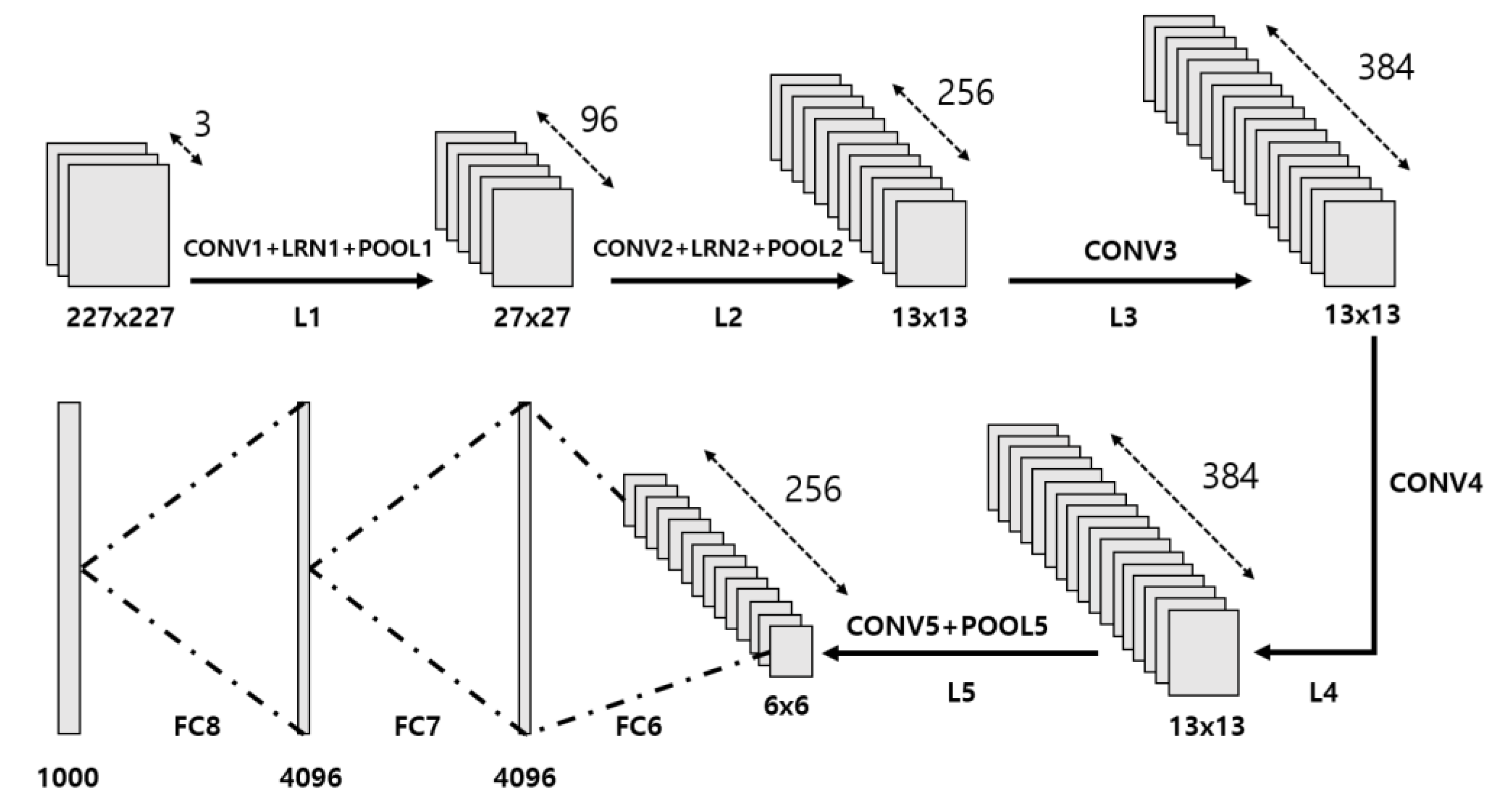
Figure 2.
Example schematic of a multilayer SPOCNN illustrating its layer-wise optical computing framework. Example schematic of a multilayer SPOCNN illustrating its layer-wise optical computing framework. LD, PD, EP, and SPLM represent the light source, photodetector, electronic processor, and smart pixel light modulator, respectively. The superscript denotes the layer number, and LD′ indicates the backward light source.
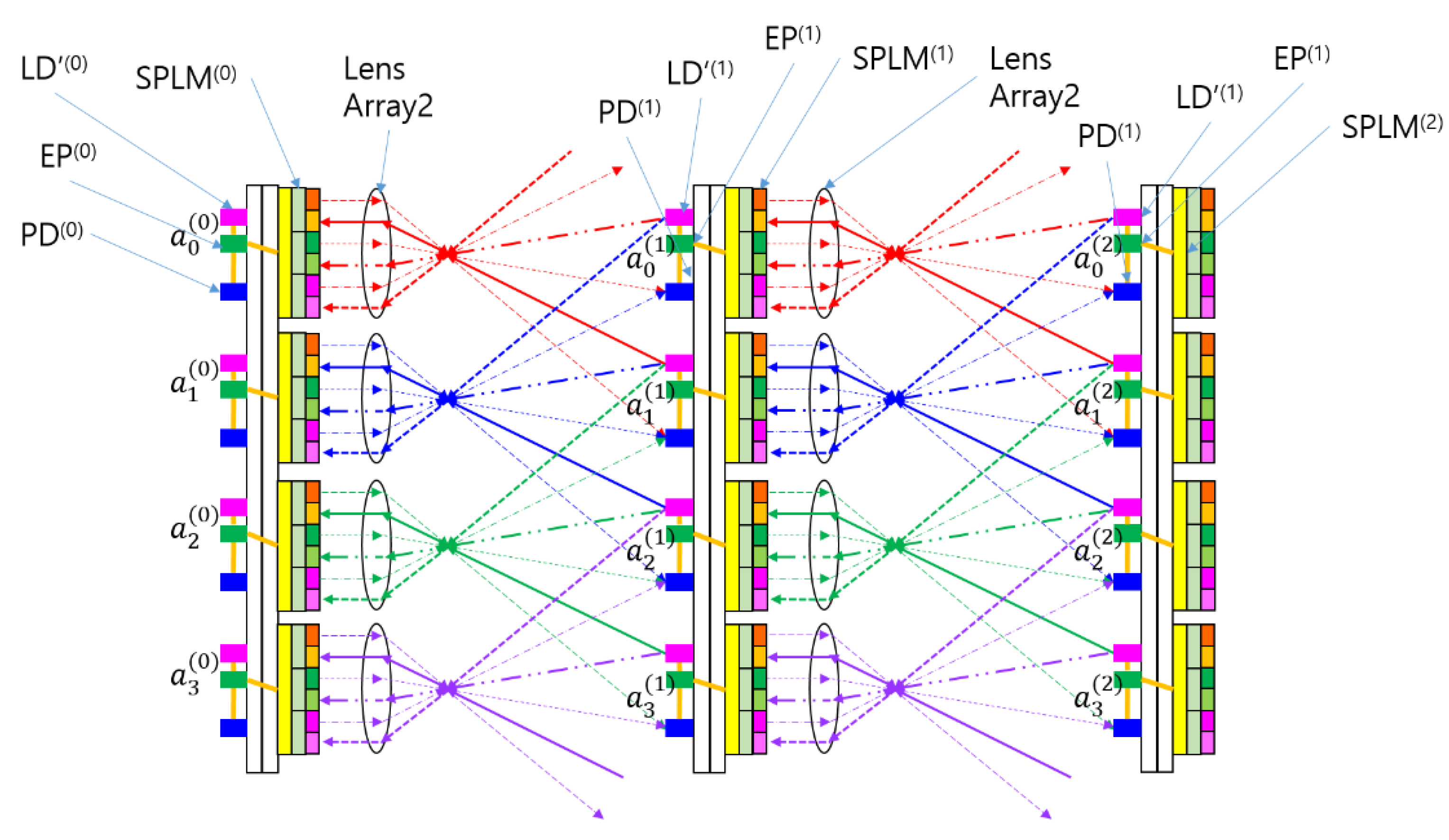
Figure 3.
Optical CNN (OCNN) with integrated crossbar switch network. (a) Schematic of a CNN incorporating a crossbar switch network. The yellow square in the crossbar switch represents memory; (b) Smart-pixel-based optical CNN (SPOCNN) with a crossbar switch network; (c) Three-dimensional view of the SPOCNN architecture illustrating crossbar switch integration. The horizontal and vertical crossbar planes are interconnected via bypass circuits or intermediate buffers, with additional buffer arrays positioned at their endpoints.
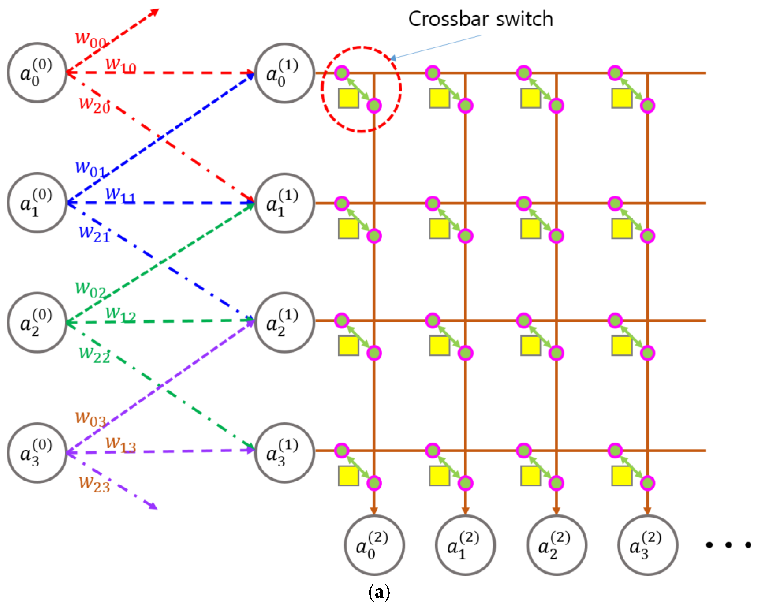
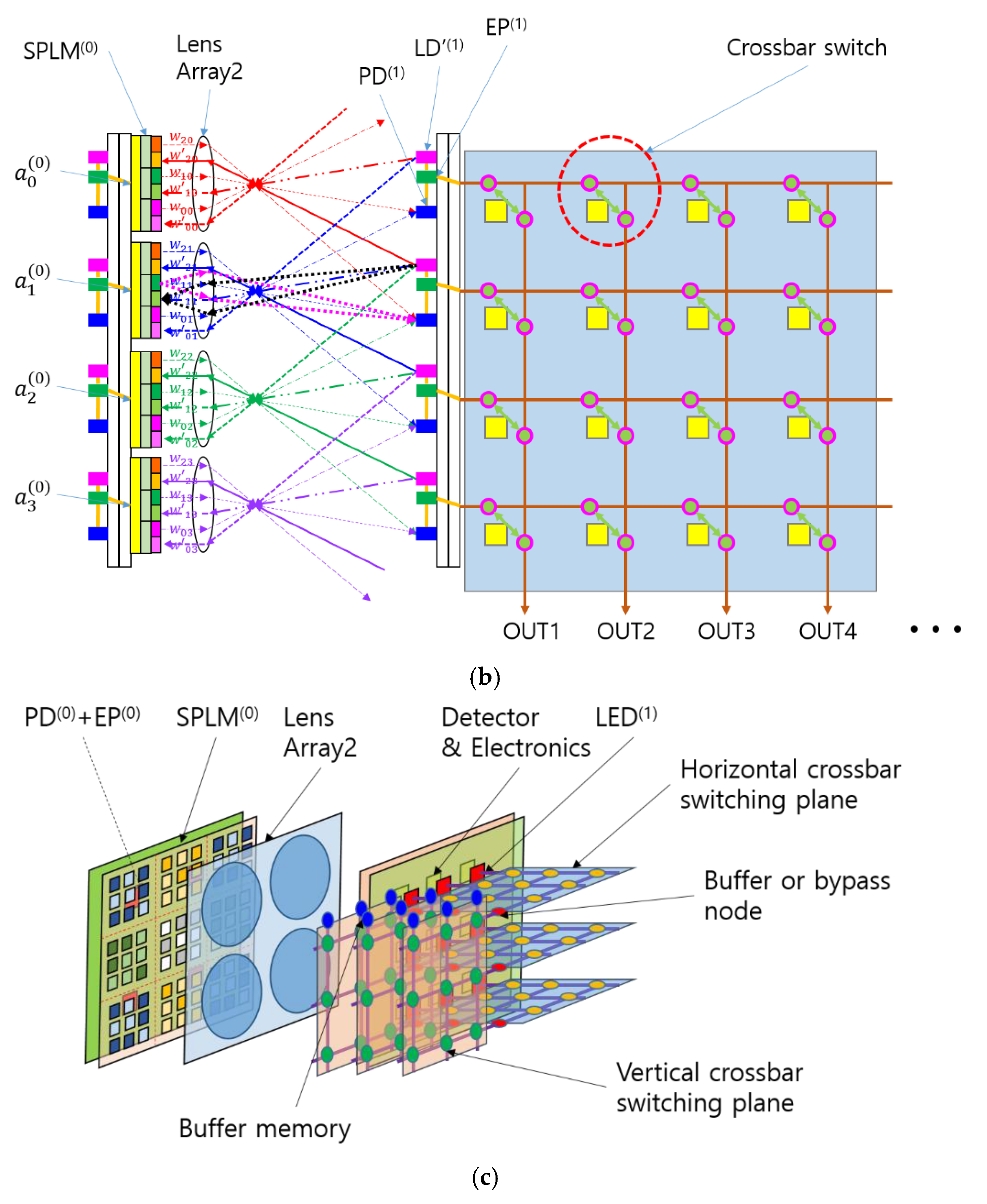
Figure 4.
Schematic diagram of a cascaded OCNN with a crossbar switch network, featuring auxiliary switches and buffers for managing three-way data flow.
Figure 4.
Schematic diagram of a cascaded OCNN with a crossbar switch network, featuring auxiliary switches and buffers for managing three-way data flow.
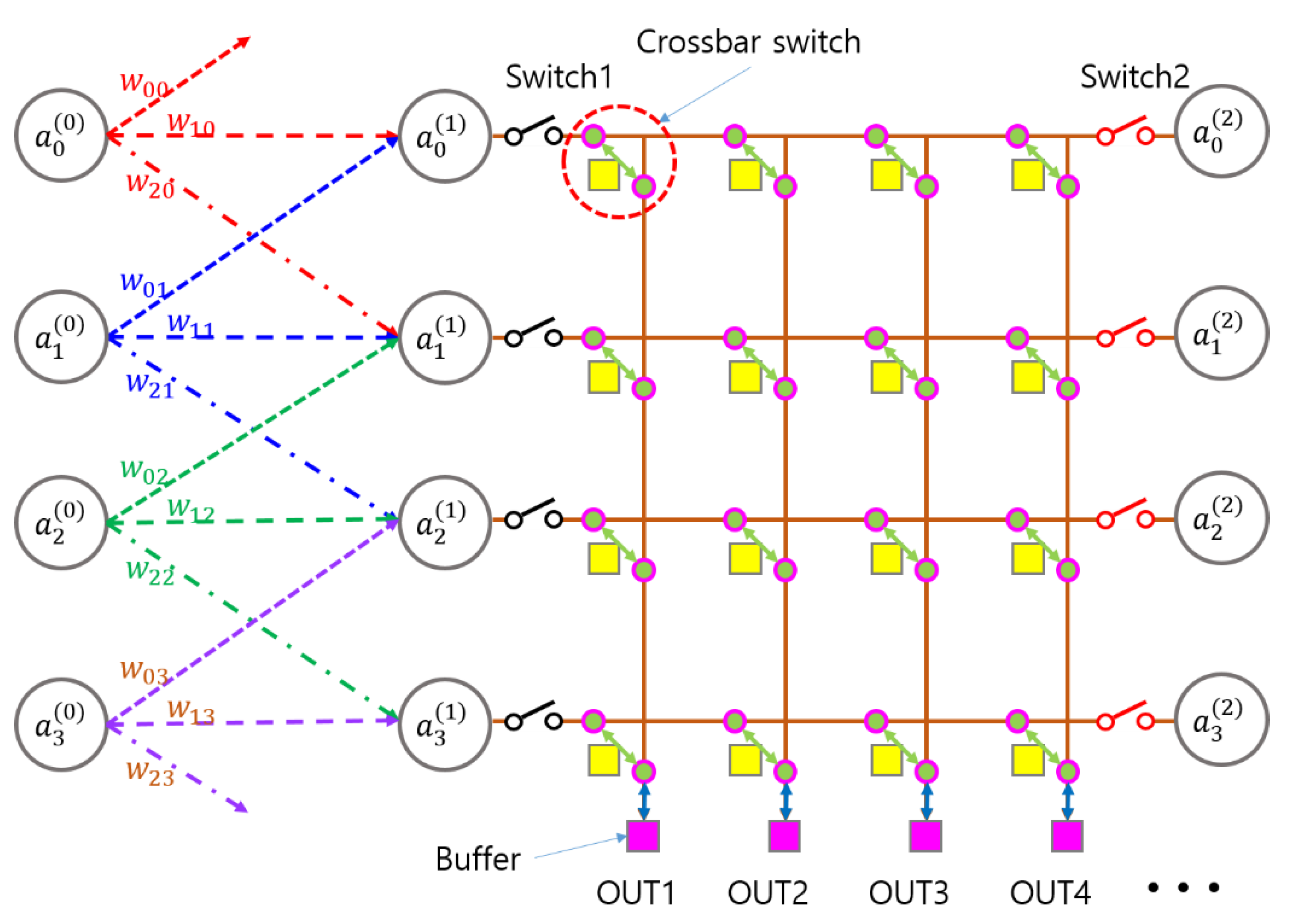
Figure 5.
Illustration of a multilayer OCNN architecture incorporating a crossbar switch network with auxiliary switches and buffers. (a) Schematic diagram with neural network nodes. (b) Schematic diagram showing the corresponding SPOCNN hardware implementation.
Figure 5.
Illustration of a multilayer OCNN architecture incorporating a crossbar switch network with auxiliary switches and buffers. (a) Schematic diagram with neural network nodes. (b) Schematic diagram showing the corresponding SPOCNN hardware implementation.
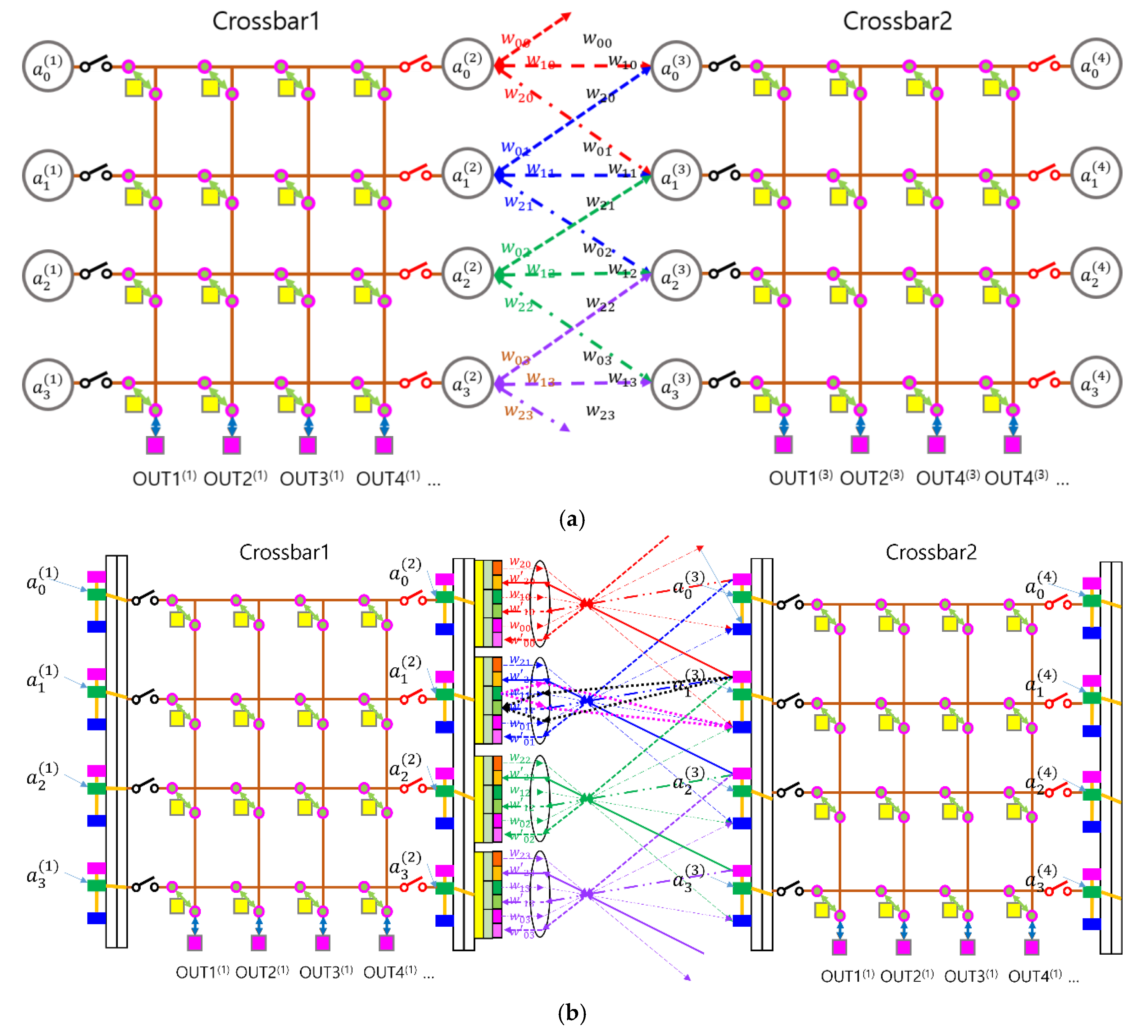
Figure 6.
Illustration of a convolution operation on feature maps using a SPOCNN integrated with a crossbar switch network, demonstrating the application of a single kernel across all feature maps.
Figure 6.
Illustration of a convolution operation on feature maps using a SPOCNN integrated with a crossbar switch network, demonstrating the application of a single kernel across all feature maps.
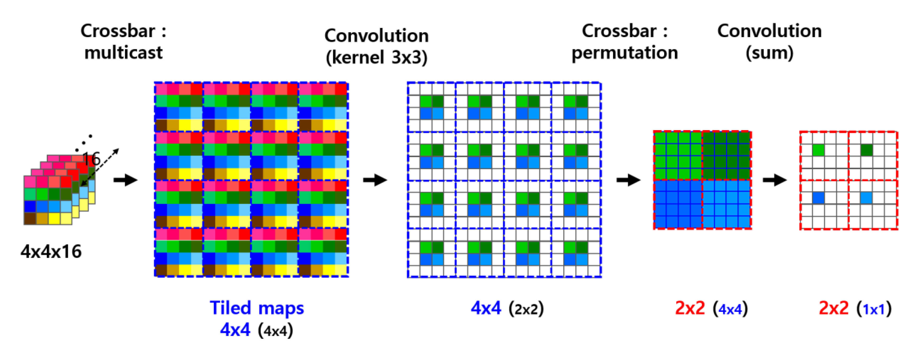
Figure 7.
Illustration of a max pooling operation on feature maps using a SPOCNN integrated with a crossbar switch network. The numbers in parentheses indicate the sets of data involved in the cumulative max operations performed up to that point. The pooling window size is 3 × 3.
Figure 7.
Illustration of a max pooling operation on feature maps using a SPOCNN integrated with a crossbar switch network. The numbers in parentheses indicate the sets of data involved in the cumulative max operations performed up to that point. The pooling window size is 3 × 3.
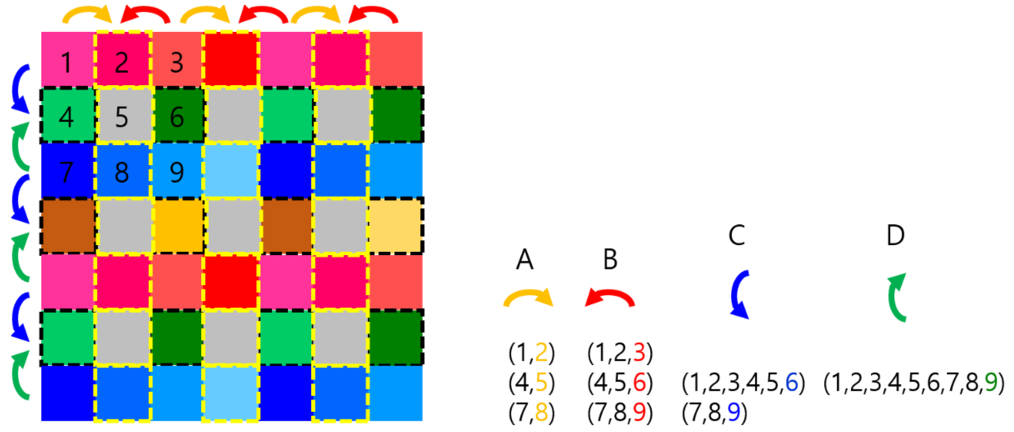
Figure 8.
Illustration of an LRN operation on feature maps using a SPOCNN integrated with a crossbar switch network. The normalization window size is 3.
Figure 8.
Illustration of an LRN operation on feature maps using a SPOCNN integrated with a crossbar switch network. The normalization window size is 3.
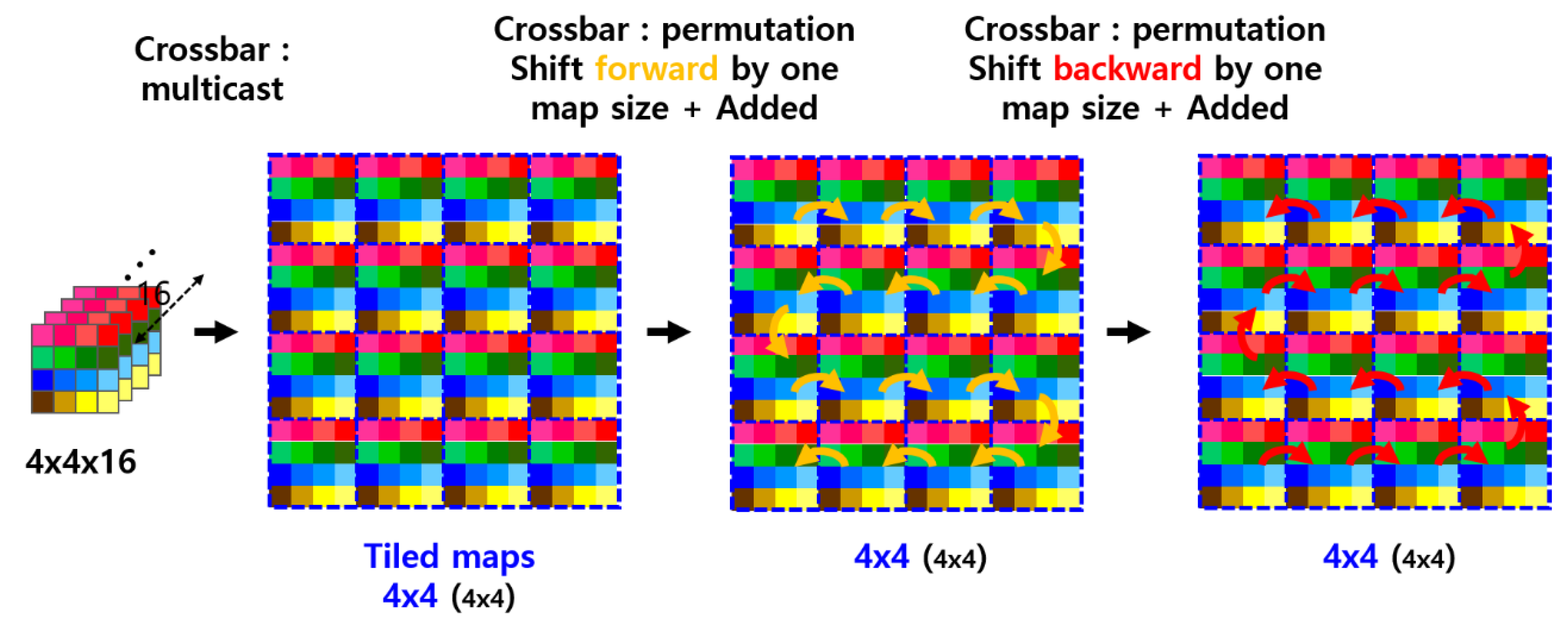

Table 1.
Summary of the full layer architecture of the AlexNet model [22], including input size, convolutional, pooling, normalization, and fully connected layers, along with their respective kernel sizes, strides, paddings, and output dimensions.
Table 1.
Summary of the full layer architecture of the AlexNet model [22], including input size, convolutional, pooling, normalization, and fully connected layers, along with their respective kernel sizes, strides, paddings, and output dimensions.
| Layer | Type | Kernel Size / Stride | Padding | Output Size | Remarks |
| Input | Input Image | - | - | 227×227×3 | RGB image |
| Conv1 | Convolution | 11×11×3 / 4 | 0 | 55×55×96 | |
| LRN1 | Normalization | - | - | 55×55×96 | Window size =5 |
| Pool1 | Max Pooling | 3×3 / 2 | 0 | 27×27×96 | |
| Conv2 | Convolution | 5×5×48 / 1 | 2 | 27×27×256 | Group split |
| LRN2 | Normalization | - | - | 27×27×256 | Window size =5 |
| Pool2 | Max Pooling | 3×3 / 2 | 0 | 13×13×256 | |
| Conv3 | Convolution | 3×3×128 / 1 | 1 | 13×13×384 | |
| Conv4 | Convolution | 3×3×192 / 1 | 1 | 13×13×384 | Group split |
| Conv5 | Convolution | 3×3×192 / 1 | 1 | 13×13×256 | Group split |
| Pool5 | Max Pooling | 3×3 / 2 | 0 | 6×6×256 | |
| FC6 | Fully Connected | - | - | 4096 | Flattened input size: 6×6×256 = 9216 |
| FC7 | Fully Connected | - | - | 4096 | |
| FC8 | Fully Connected | - | - | 1000 | Softmax output |
Table 2.
Instruction cycle breakdown for each stage of the AlexNet architecture implemented using the SPOCNN framework with integrated crossbar switch networks.
Table 2.
Instruction cycle breakdown for each stage of the AlexNet architecture implemented using the SPOCNN framework with integrated crossbar switch networks.
| Layer / Operation | Description | Instruction Cycles |
|---|---|---|
| RGB Multicast | Multicast RGB images to 96 kernels (2 per channel × 3) | 6 |
| Conv1 | Convolution with 11×11 kernel, stride 4 | 3 |
| LRN1 | Local Response Normalization, window size 5 | 5 |
| Pool1 | Max pooling with 3×3 window, stride 2 | 8 |
| Rearrangement after Pool1 | Data formatting using multicast (2 instructions) | 2 |
| Conv2 to Pool2 | Conv2, LRN2, and Pool2 combined | 16 |
| Conv3 to Conv5 | Convolution layers 3 to 5 | 12 |
| Pool5 | Max pooling layer | 8 |
| Intermediate Rearrangements | 4 rearrangement operations (2 cycles each) | 8 |
| FC6 to FC8 | Three fully connected layers (SPBONN) | 3 |
| Total | Total instruction cycles required | 71 |
Disclaimer/Publisher’s Note: The statements, opinions and data contained in all publications are solely those of the individual author(s) and contributor(s) and not of MDPI and/or the editor(s). MDPI and/or the editor(s) disclaim responsibility for any injury to people or property resulting from any ideas, methods, instructions or products referred to in the content. |
© 2025 by the authors. Licensee MDPI, Basel, Switzerland. This article is an open access article distributed under the terms and conditions of the Creative Commons Attribution (CC BY) license (http://creativecommons.org/licenses/by/4.0/).
Copyright: This open access article is published under a Creative Commons CC BY 4.0 license, which permit the free download, distribution, and reuse, provided that the author and preprint are cited in any reuse.


