A Conceptual Study of Rapidly Reconfigurable and Scalable Optical Convolutional Neural Networks Based on Free-Space Optics Using a Smart Pixel Light Modulator

1. Introduction

In recent years, deep learning algorithms, particularly artificial neural networks, have significantly advanced fields such as image recognition, speech processing, and natural language understanding [1,2]. Among these, convolutional neural networks (CNNs) stand out as one of the most effective deep learning architectures for image and video processing tasks [3]. CNNs are designed to automatically identify and extract key features like edges, corners, and textures from images, enabling classification into distinct categories. This is achieved through convolutional operations, where filters (kernels) of various sizes are applied to the input image. The results are then processed through pooling, nonlinear activation functions, and subsequent layers of convolution.

Despite their effectiveness in solving classification and recognition tasks, CNNs demand extensive computational resources, especially when handling large image datasets or kernels. For instance, convolving an image with dimensions n × n pixels using a k × k kernel requires computations proportional to n² × k². This computational load increases significantly with deeper networks, leading to latency and high power consumption during forward inference in pretrained models. While graphics processing units help mitigate some latency challenges, real-time processing remains a bottleneck for large-scale systems [4].

To address these challenges, researchers have turned to free-space optics for implementing CNNs, leveraging their inherent parallelism and energy efficiency. Traditional optical convolutional neural networks (OCNNs) often use the well-established 4f correlator system [5,6,7,8], which exploits the Fourier transform for computation [9]. However, this approach has notable drawbacks. First, the scalability of the input image is constrained by the finite space-bandwidth product (SBP) of the lens used in Fourier transformations [5], which is further limited by geometric aberrations. Second, latency arises due to the slow operation of spatial light modulators (SLMs) used to generate coherent input arrays. Current SLMs are serially addressable and operate at speeds significantly slower than electronic components, typically in the tens of kilohertz range [10,11], causing delays that hinder the parallel processing benefits of optical systems. This slow refresh rate becomes even more problematic in multilayer neural networks, where outputs from one layer serve as inputs to the next. Reconfiguring the SLM pixels for every layer transition adds further delays, impacting overall throughput.

Another critical limitation of 4f correlator-based systems is the difficulty of reconfiguring kernel patterns. Since the kernel representation in such systems is the Fourier transform of the actual pattern, additional computation is required to generate and update the kernel, leading to further delays.

To address these limitations, a novel scalable optical convolutional neural network (SOCNN) architecture was previously proposed, leveraging free-space optics combined with Köhler illumination, lens arrays, and a SLM [12]. This SOCNN builds upon the previously introduced linear combination optical engine (LCOE) [13], adapting it to include CNN-specific functionalities. While the LCOE was designed for full interconnections, the SOCNN focuses on partial connections, enabling scalability to accommodate input arrays of virtually unlimited size.

The SOCNN resolves many challenges associated with the traditional 4f correlator system. It eliminates the scalability limitations of input arrays and reduces crosstalk noise through the use of Köhler illumination [14,15]. Additionally, because it does not rely on a coherent light source or an SLM, it avoids the substantial delays caused by loading input data into the SLM—an issue particularly problematic in multilayer configurations of the traditional 4f correlator system. Moreover, unlike the 4f correlator system, the SOCNN does not require additional computation for updating neural network weights, as the transmission values in the SOCNN are directly proportional to the weights. This feature offers a significant advantage in applications where weights change dynamically, such as during training.

Although the SOCNN offers numerous benefits, it has inherent drawbacks due to its reliance on SLMs. As noted earlier, current SLMs are slow and serially addressable, resulting in significant delays during updates and reconfigurations. Although this does not impede optical parallelism in inference applications, it becomes a significant challenge in scenarios requiring rapid weight reconfiguration. For example, convolving the same input data with different kernel sets necessitates frequent weight updates.

To overcome these challenges, this study proposes a smart-pixel-based optical convolutional neural network (SPOCNN) that replaces the SLM in the SOCNN architecture with a smart pixel light modulator (SPLM) [16,17]. The adoption of SPLMs leverages current optoelectronic technology to enhance the speed of weight updates, enabling rapid reconfigurability. This improvement extends the application scope of SOCNNs. A similar approach has been previously explored in smart-pixel-based optical neural networks (SPONNs) [18], where SPLMs were used in place of SLMs for faster reconfiguration in systems such as the LCOE and bidirectional optical neural network (BONN) [19].

Additionally, we propose a bidirectional version of the SPOCNN, known as smart-pixel-based bidirectional optical convolutional neural networks (SPBOCNN). Its bidirectional design enables backward data flow, which can be advantageous for learning algorithms. Furthermore, it enables the implementation of two-mirror-like optical neural networks [18,19] for convolution, allowing data to transfer between two layers, effectively emulating multiple layers and reducing hardware requirements. Lastly, the integration of SPLM enhances the scalability of the OCNN by utilizing its memory capabilities without adding hardware complexity, making the system more versatile and adaptable for real-world applications. The subsequent sections will provide an analysis of the optical structures and their performance

2. Materials and Methods

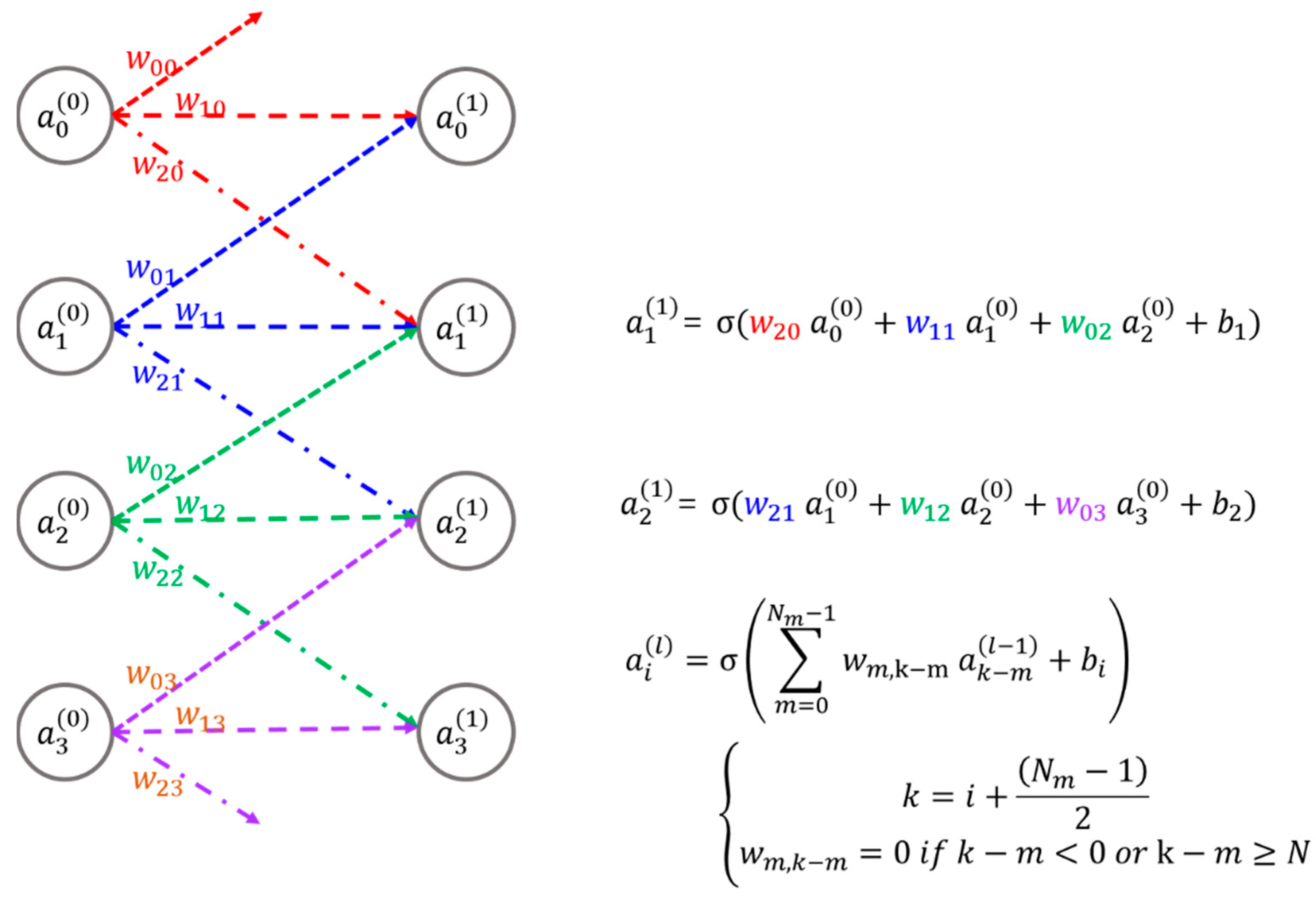
To comprehend the structure of the proposed SPOCNN, it is important to first understand the basic concept of a CNN. Figure 1 illustrates an example of a CNN, which includes four input nodes, four output nodes, and their corresponding synaptic connections, along with the mathematical representations of these connections. A CNN functions by receiving signals at its input nodes, transmitting them through weighted synaptic connections to the output nodes, and then producing the final output. These synaptic weights, represented mathematically, determine the strength of each connection. Unlike fully connected optical neural networks like the LCOE, CNNs utilize localized or partial connections, where the weights assigned to these connections are referred to as kernels.

Figure 1. Illustration of a basic CNN along with its mathematical representation: $a_i^{\left(l\right)}$​ denotes the i-th input or output node in the l-th layer; $w_{ij}$​ represents the weight linking the j-th input node to the i-th output node; $b_i$ stands for the bias associated with the i-th node; N refers to the size of the input array, while N_m​ specifies either the kernel size or the number of weights connected to an input or output node; and σ represents the sigmoid activation function.

Figure 1. Illustration of a basic CNN along with its mathematical representation: $a_i^{\left(l\right)}$​ denotes the i-th input or output node in the l-th layer; $w_{ij}$​ represents the weight linking the j-th input node to the i-th output node; $b_i$ stands for the bias associated with the i-th node; N refers to the size of the input array, while N_m​ specifies either the kernel size or the number of weights connected to an input or output node; and σ represents the sigmoid activation function.

The previous SOCNN architecture [12] demonstrates outstanding optical parallelism and unlimited scalability of input node sizes with fixed weights, making it especially well-suited for inference tasks. However, it has limitations in applications that require applying the same input data to different sets of weight data, due to its relatively slow update rate. While SLMs provide reconfigurability and programmability, their current switching speeds are restricted to a few kilohertz [10,11], leading to delayed computations and a significant reduction in throughput when weight updates are necessary during processing.

To address the limitations of SLMs in such scenarios, two potential solutions exist. The first involves developing a high-speed SLM array, such as those based on absorption modulators. However, this approach demands substantial time, resources, and financial investment. Alternatively, a more practical solution lies in leveraging existing technologies, such as smart pixels [16,17], which integrate a detector, light source, and EP into a single chip. Advances in optoelectronic packaging have made it possible to hybridize these components into arrays. Furthermore, the EP can perform multiple functions, including memory operations, enabling ONNs to be more programmable and intelligent compared to systems relying solely on SLMs.

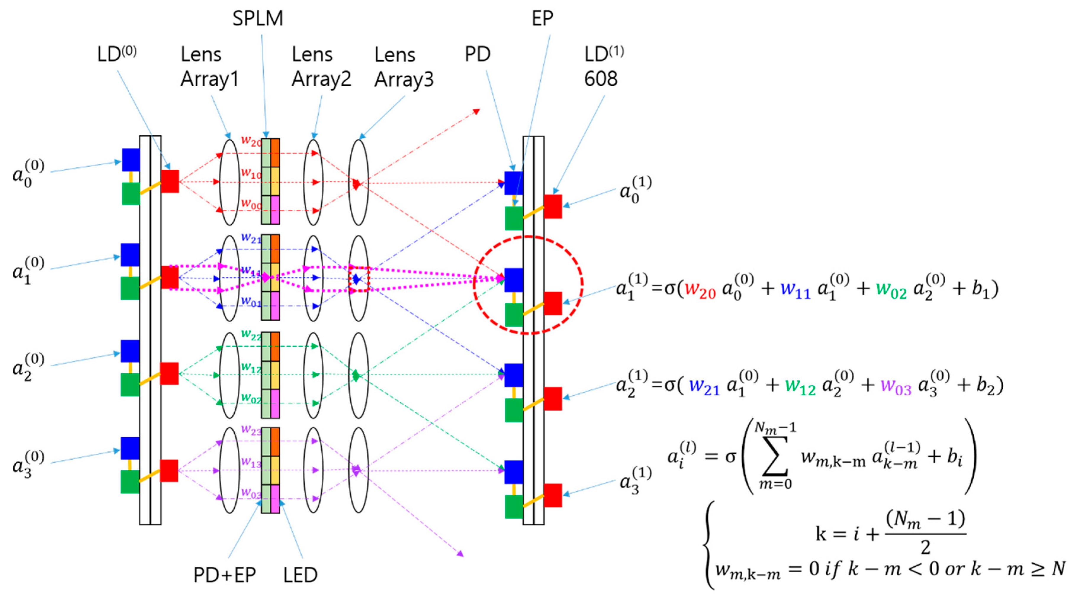
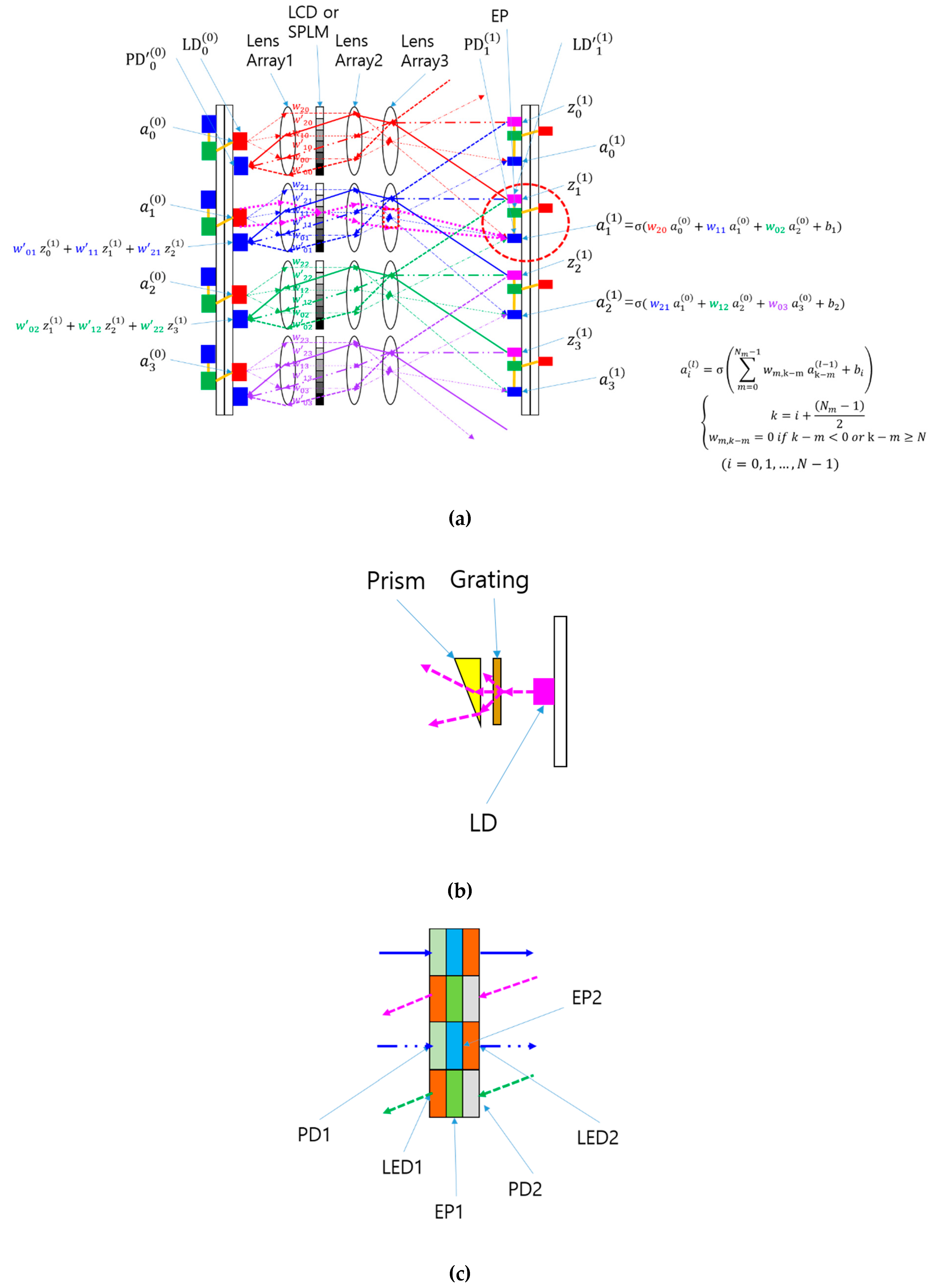
Figure 2 provides a visual representation of the SPOCNN concept introduced in this study. The CNN depicted in Figure 1 has been converted into a hardware configuration comprising laser diodes (LDs), lenses, an SPLM, detectors, and associated electronics. In this design, the input node is substituted with an LD that emits three rays directed at lens array 1. This setup supports the use of either a multimode vertical-cavity surface-emitting laser (VCSEL) or a light-emitting diode (LED) as the LD, as the system is designed to handle incoherent light sources—unlike the conventional 4f correlator system, which typically requires coherent light.

Lens Array 1 collimates incoming rays and directs them to the SPLM, where each smart pixel modulates the light based on a pre-trained kernel in the CNN. The modulated rays exiting the SPLM pass through Lens Array 2, which focuses them and adjusts their angles according to the distance between the SPLM pixel and the optical axis of each individual lens within the array.

A detector aggregates the optical power from rays arriving at various angles, originating from multiple neighboring LDs or inputs configured with preset weights. The resulting summed light mathematically represents the convolution of the input signals with the kernel defined by the weights. This architecture enables SPOCNNs to perform computations simultaneously and, critically, in a single step at the speed of light. This type of rapid computation aligns with what is termed "inference" in the neural network domain. The rapid reconfigurability of SPOCNNs makes them suitable for a wider range of applications beyond inference compared to SOCNNs.

Analyzing the optical system depicted in Figure 2(a), Lens 2 and Lens 3 function as a relay imaging system. Typically, the SPLM is placed at the focal plane of Lens 2, while the detector is positioned at the focal plane of Lens 3. This setup ensures that the SPLM and detector planes are optically conjugated, meaning each pixel on the SPLM is imaged onto a corresponding point on the detector plane. By establishing this conjugate relationship, the illumination for each ray is well-defined, minimizing channel crosstalk.

Furthermore, when an LD is located at the focal plane of Lens 1, Lens 1 and Lens 2 act as a relay system to form an image of the LD at Lens 3. Collectively, the lens arrangement in Figure 2(a) constitutes a Köhler illumination system [14,15]. In this system, the dotted magenta lines represent the chief rays from the condenser's perspective, whereas they represent the marginal rays from the projection's perspective. The red dotted rectangle at Lens 3 signifies the image of the light source. Lens 2 and Lens 3 jointly form the projection lens within the Köhler illumination setup. Meanwhile, the rays emitted from the LDs uniformly spread across the detector plane, ensuring even illumination.

The SPOCNN architecture is fundamentally the same as the SOCNN [12], with the primary distinction being the use of SPLM instead of SLM. To achieve higher modulation speeds, multi-mode VCSELs can be used instead of LEDs, which have limited modulation capabilities [19,20,21]. The SPLM, illustrated in Figure 2, is composed of a photodetector (PD), an electronic processor (EP), and a light-emitting diode (LED). The PD captures incoming light, converts it into an electrical signal, and transmits it to the EP within the SPLM. The EP amplifies the signal based on the weight value stored in its integrated memory. This amplified signal is then sent to the LED, which emits light proportional to the input and weight. Together, the PD, EP, and LED form a single pixel, where these pixels are locally connected, except during the program loading phase. Once the program is loaded, the pixel array operates autonomously, preserving the system’s parallelism. Each pixel effectively functions as a compact signal repeater.

Thanks to its electronic components, the modulation speed of the SPLM surpasses several hundred megahertz, significantly outpacing typical SLM technologies such as liquid crystal displays and micro-electro-mechanical systems [10,11]. While the SPLM introduces two additional conversion steps between optical and electronic signals, the associated delay is minimal, amounting to only a few nanoseconds [17]. Nevertheless, the substantial benefits of the SPLM’s high modulation speed far outweigh this minor delay, particularly in numerous practical applications, as discussed in the introduction.

The primary distinction between the SPOCNN and the earlier SPONN [18] lies in their connection structures. In the SPOCNN, each input is connected to a relatively small number of output nodes, whereas the SPONN employs a fully interconnected architecture. This feature of partial connectivity significantly alleviates limitations on the input array size. Unlike the traditional 4f correlator system, the SPOCNN does not impose a theoretical limit on the size of the input array. However, the size of the kernel array is constrained due to the SBP limitations imposed by the imaging properties of the lenses used for SPLM pixel projection. This topic will be further elaborated in the discussion section.

Figure 2. An example of an SPOCNN utilizing free-space optics with lens arrays and an SPLM: Schematic representation and corresponding mathematical formula. The SPLM used in the SPOCNN includes smart pixels comprising a photodetector (PD), electronic processing (EP), and a light-emitting diode (LED). The smart pixels receive light input and emit output light proportional to the weight value stored in the EP memory. The LD can be either a laser diode or an LED.

Figure 2. An example of an SPOCNN utilizing free-space optics with lens arrays and an SPLM: Schematic representation and corresponding mathematical formula. The SPLM used in the SPOCNN includes smart pixels comprising a photodetector (PD), electronic processing (EP), and a light-emitting diode (LED). The smart pixels receive light input and emit output light proportional to the weight value stored in the EP memory. The LD can be either a laser diode or an LED.

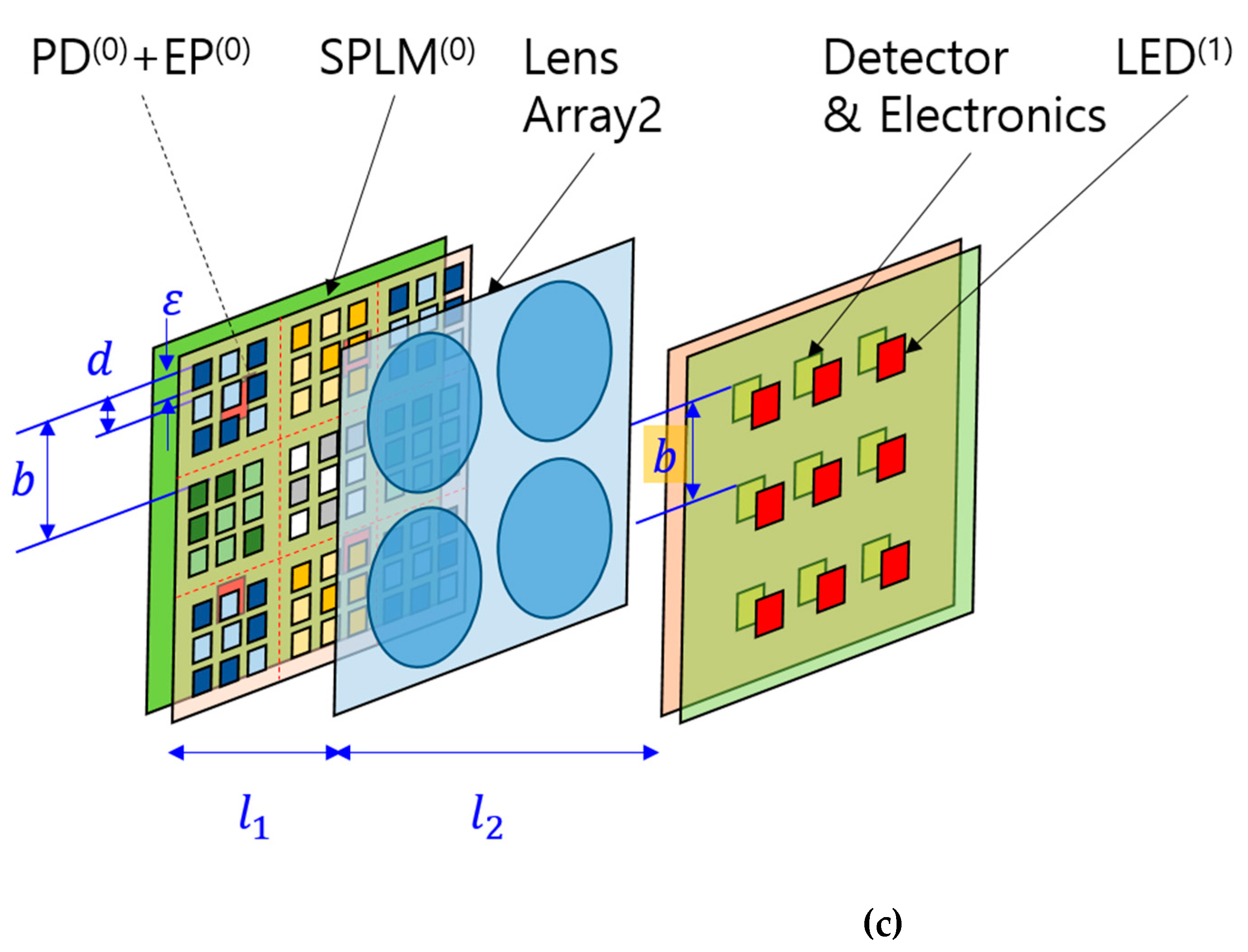
In the setup illustrated in Figure 3(a), the number of smart pixels associated with each input node corresponds to the number of output nodes connected to that input. These smart pixels, grouped as subarrays within the SPLM, represent the receptive field of the output nodes. Although the SPOCNN shown in Figure 3(a) is depicted in one dimension, it can easily be extended to a two-dimensional input-output structure. For example, if the subarray consists of a 3 × 3 pixel arrangement with a pixel spacing of d, and the detector spacing is b, the projection system’s magnification, given by as l₃ /l₂, must match b/d. Here, l₂ and l₃ represent the distances from Lens2 to the SPLM and from Lens2 to the detectors, respectively.

If a single kernel occupies an 8 × 8 pixel area on the SPLM, it can connect to 64 output nodes. For instance, an SPLM with a resolution of 3840 × 2160 pixels can support up to 480 × 270 input nodes, equating to 129,600 inputs. Considering the parallel processing capability of the SPOCNN, its performance is directly tied to the resolution of the SPLM. For a system with N × N inputs and an M × M kernel, the SPOCNN can perform N² × M² multiplications and N² × (M² − 1) additions in a single step. If the full resolution of the SPLM is utilized, (N × M)² matches the total number of pixels available. Furthermore, the high refresh rate of the SPLM—reaching several hundred megahertz [17]—makes the SPOCNN well-suited for applications requiring rapid weight updates. Additionally, since the SPLM transmission is directly proportional to the kernel weight, there is no need for additional Fourier transform calculations, unlike the 4f correlator system. This feature highlights the SPOCNN's potential as a fast reconfigurable OCNN for future applications.

After the optical processing stage, the detector converts the light into an electrical signal. Subsequent steps, including signal amplification, bias addition, and nonlinear operations (e.g., sigmoid, ReLU, local response normalization, and max-pooling), are carried out electronically. Electronics are better suited for these nonlinear computations due to their inherent characteristics. However, to prevent interconnection bottlenecks, connections between distant electronic components should be minimized. As long as the electronics within the detector-side smart pixels remain localized and distributed, the system’s optical parallelism remains intact.

The SPOCNN is inherently a cascading architecture, allowing for straightforward extension in the direction of beam propagation. The signal from each output node directly connects to the corresponding input of the subsequent layer. In this configuration, each neuron in the artificial neural network comprises a detector, its associated electronics, and a laser diode in the next layer. For a system with L layers, N² × M² × L computations can occur simultaneously in a single step, significantly boosting the SPOCNN's throughput for continuous input.

Additionally, another difference between SPOCNN and SOCNN is that the LED output in the SPLM produces diverging rays, whereas the SLM maintains collimated light. This divergence can be minimized by placing a small lens directly after the LED. However, the diverging beam does not compromise the performance of the SPOCNN. This is because the SPLM plane is optically conjugate to the detector plane in the SPOCNN, as aligned through Lens2 and Lens3. Consequently, the LED’s image on the SPLM is accurately projected onto the detector plane, regardless of the LED's divergence angle.

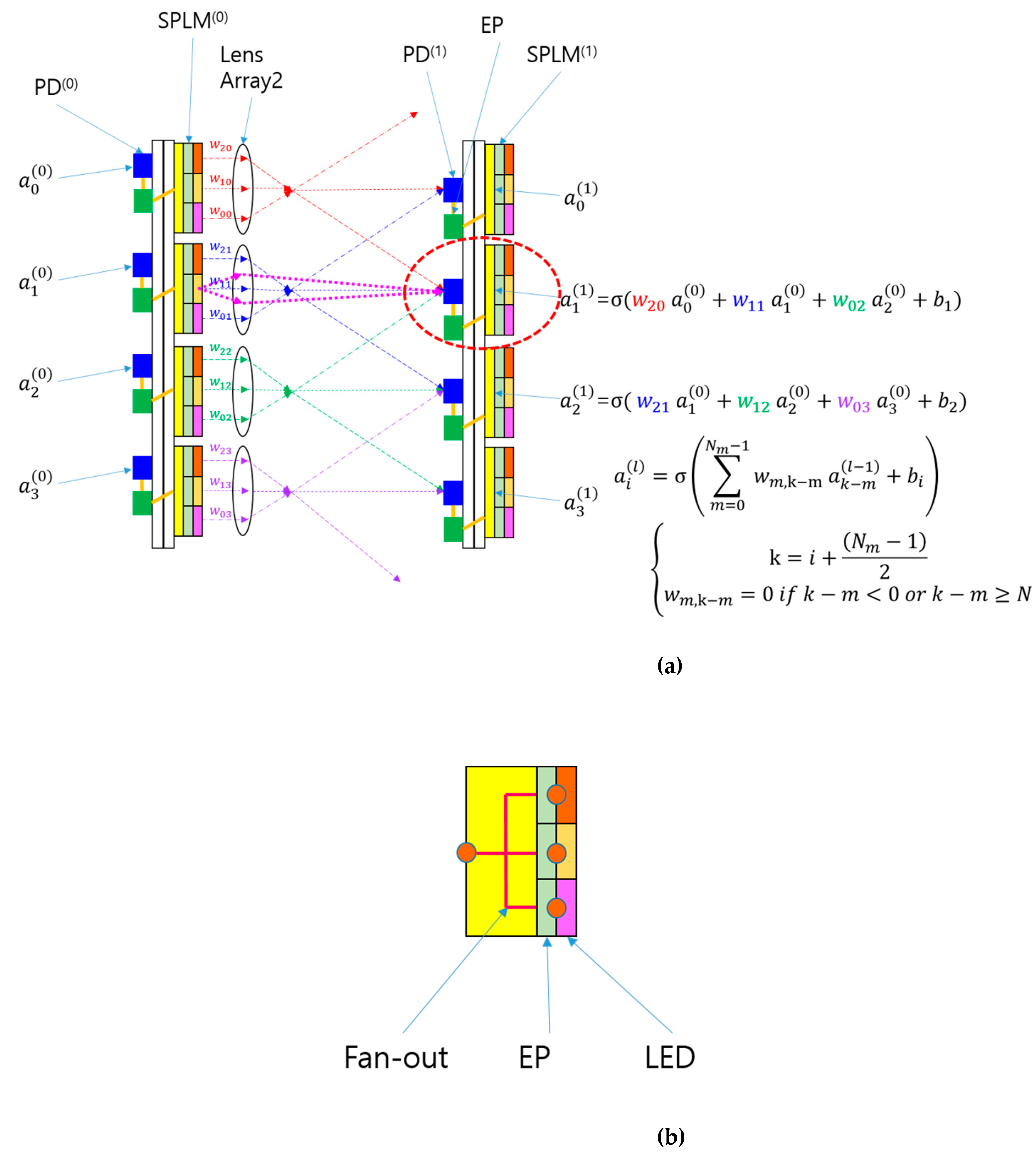
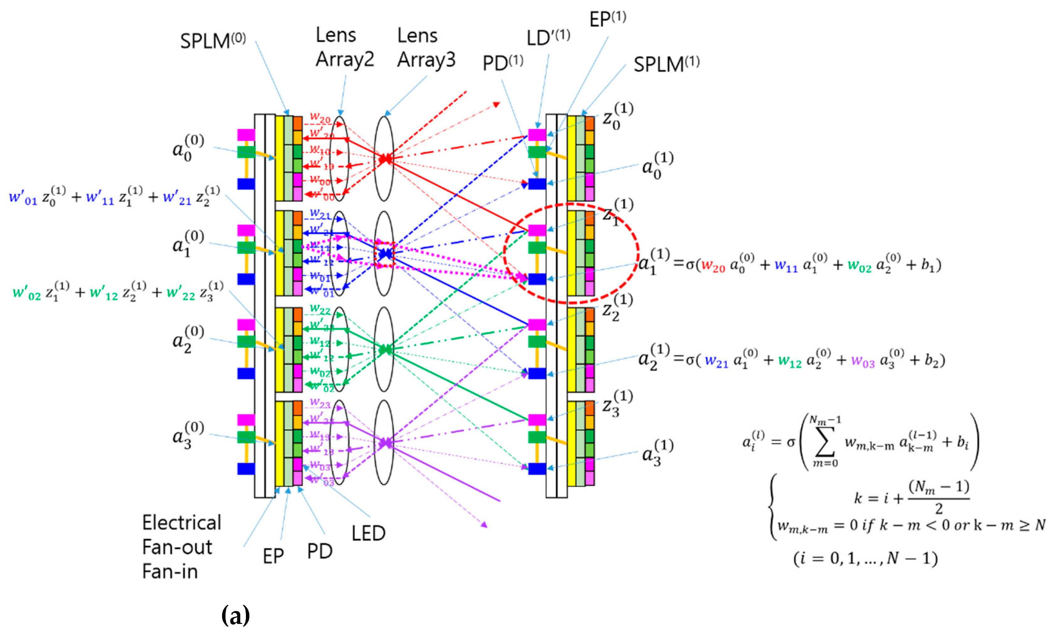
The SPOCNN design can be further streamlined by replacing LD⁽⁰⁾ and Lens1 with an electrical fan-out, as depicted in Figure 3(a). A detailed illustration of the electrical fan-out is provided in Figure 3(b). In the original setup, the light source and Lens1 function as an optical distributor for the input signal. In contrast, the electrical fan-out shown in Figure 3a,b serves as an alternative distributor in the electrical domain. This configuration employs a straightforward wiring scheme that connects the output of the preceding layer to the inputs of the SPLM pixels in the subsequent layer. By adopting this approach, wiring complexity and electromagnetic interference are significantly reduced, simplifying the overall system.

The removal of LD⁽⁰⁾ and Lens1 not only simplifies the optical design but also eliminates the need for Köhler illumination. In the original design, Köhler illumination involves Lens1 and Lens2 forming a condenser system, while Lens2 and Lens3 comprise a projection system, as shown in Figure 2. By removing the condenser system and retaining only the projection system, additional simplifications can be achieved, as shown in Figure 3(a). In this revised configuration, Lens2 and Lens3 can be merged into a single lens element, reducing space requirements and easing optical alignment challenges. This integration also leads to cost savings and further streamlines the system. Each layer in the SPOCNN is composed of an input smart-pixel array, a lens array, and an output detector array connected to a smart-pixel array. This simplified SPOCNN closely resembles the convolutional version of a lens array processor [22], with the key difference being the incorporation of smart pixels.

The replacement of SLMs with SPLMs offers substantial advantages by significantly simplifying the architecture and potentially lowering fabrication complexity and costs in the future. A 3D representation of the SPONN system is presented in Figure 3(c). This modular architecture supports cascading and is well-suited for implementing multilayer ONNs, similar to the LCOE design.

Figure 3. The simplified version of the SPOCNN utilizing electrical fan-out: (a) Schematic representation and corresponding mathematical formula. Additionally, Lens 2 and Lens 3 in Figure 2 are combined into a single lens; (b) The SPLM used in the SPOCNN, where the electrical fan-out connects the input nodes to individual pixels in the SPLM. EP represents the electronic processing for each pixel, which includes memory and is connected to the LED output; (c) A three-dimensional view of the system with 3 × 3 inputs and 3 × 3 outputs. ε represents the size of the light source in the SPLM, while b, and d indicate the spacing between detectors (or subarrays) and smart pixels, respectively. l₁ and l₂ denote the distances from Lens2 to the SPLM and the detector, respectively.

Figure 3. The simplified version of the SPOCNN utilizing electrical fan-out: (a) Schematic representation and corresponding mathematical formula. Additionally, Lens 2 and Lens 3 in Figure 2 are combined into a single lens; (b) The SPLM used in the SPOCNN, where the electrical fan-out connects the input nodes to individual pixels in the SPLM. EP represents the electronic processing for each pixel, which includes memory and is connected to the LED output; (c) A three-dimensional view of the system with 3 × 3 inputs and 3 × 3 outputs. ε represents the size of the light source in the SPLM, while b, and d indicate the spacing between detectors (or subarrays) and smart pixels, respectively. l₁ and l₂ denote the distances from Lens2 to the SPLM and the detector, respectively.

3. Results

The use of the SPLM instead of the SLM in an SOCNN [12] can also be adapted for application in BONN [19], as depicted in Figure 4(a). In this smart pixel-based bidirectional OCNN (SPBOCNN) architecture, the SPLM takes over the role previously held by the SLM, modulating light traveling in both forward and backward directions based on the neural network’s weight values. With the help of Lens2 and Lens3, the SPLM pixels' images are projected onto the detector plane or the second substrate, which also houses light sources (${LD\text{'}}_1^{\left(1\right)}$) to facilitate backward light propagation, as shown in Figure 4(b). These backward light sources may consist of laser diodes combined with a grating and prism for beam property control. The beams passing through the SPLM are focused onto PDs (${PD\text{'}}_0^{\left(0\right)}$) on the first substrate, maintaining compatibility with the backward propagation process. Even with the replacement of the SLM by the SPLM, the core BONN structure remains intact, with a significant enhancement in modulation speed.

The SPLM’s ability to operate at modulation speeds of several hundred megahertz allows the neural network’s weight-refresh rates to reach similar levels [17]. The EP memory in the SPLM quickly sends updated weight values to the amplifier in just a few nanoseconds. This rapid weight-refresh capability resolves the primary limitations associated with the slow modulation speed of SLMs in previous BONN implementations. By introducing SPLM, practical realization of the backpropagation algorithm and the two-mirror-like BONN (TMLBONN) [19] configuration becomes feasible without requiring the development of new, high-speed SLM arrays. Detailed discussions on the implementation of backpropagation in BONN and the benefits of TMLBONN within this framework can be found in reference [19].

The SPLM utilized in this BONN differs from those shown in Figure 2 and Figure 3, as detailed in Figure 4(c). To enable bidirectional modulation, the SPLM pixels are categorized into two groups. One group manages forward light propagation and includes PD1 on the left and LED2 on the right of the same pixel, linked through EP2. The other group handles backward propagation, incorporating PD2, EP1, and LED1 within a pixel to modulate light in the reverse direction. LED1 can also feature a microprism or lens to adjust beam divergence and emission angles, enhancing control and performance for bidirectional optical neural network operations.

Figure 4. An example of a SPBOCNN: (a) A schematic of the SPBONN and the associated mathematical formulas. $a_i^{\left(l\right)}$ represents the i-th input or output node in the l-th layer. $w_{ji}$ denotes the weight connecting the i-th input to the j-th output in the forward direction, while ${w\text{'}}_{ji}$​ represents the weight in the backward direction. The thin lines represent the light paths in the forward direction, while the thick lines represent those in the backward direction; (b) light source for the backward direction; (c) schematic of the smart pixel light modulator used for the SPBCONN.

Figure 4. An example of a SPBOCNN: (a) A schematic of the SPBONN and the associated mathematical formulas. $a_i^{\left(l\right)}$ represents the i-th input or output node in the l-th layer. $w_{ji}$ denotes the weight connecting the i-th input to the j-th output in the forward direction, while ${w\text{'}}_{ji}$​ represents the weight in the backward direction. The thin lines represent the light paths in the forward direction, while the thick lines represent those in the backward direction; (b) light source for the backward direction; (c) schematic of the smart pixel light modulator used for the SPBCONN.

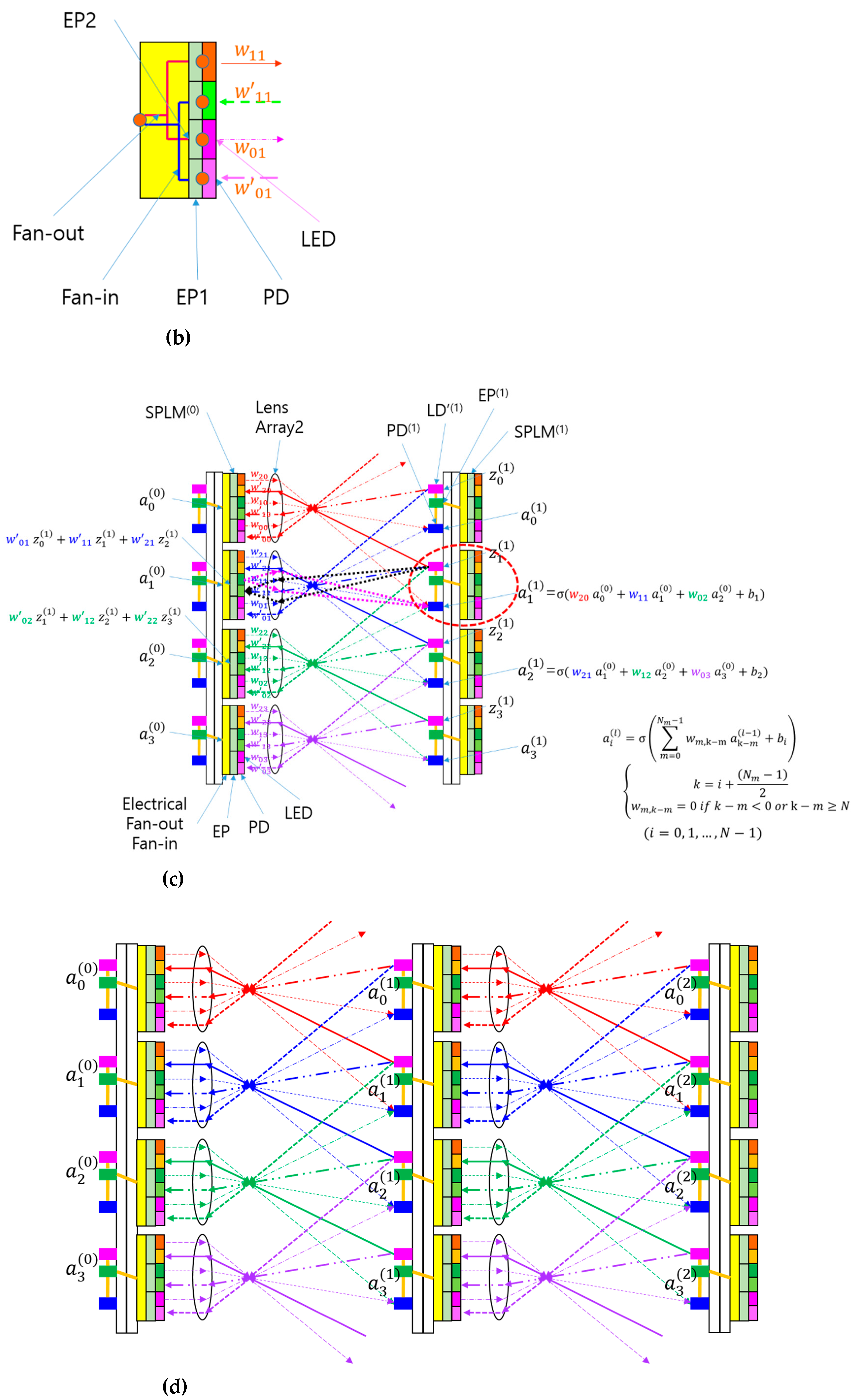
Similar to the simplification process from Figure 2 to Figure 3, the SPBOCNN design in Figure 4 can be streamlined into the configuration shown in Figure 5(a) by replacing the optical input distribution, previously handled by Lens1, with electrical fan-in and fan-out mechanisms. The updated SPBOCNN architecture, shown in Figure 5(a), includes an SPLM, lenses, smart pixels on the first substrate, and detectors on the second substrate. While retaining the bidirectional data flow, this design significantly reduces the complexity of the hardware.

An electrical fan-in is introduced to facilitate analog summation of optical signals for backward data propagation, as illustrated in Figure 5(b). The SPLM’s EPs transform the output signals into electrical current, which is then aggregated by the fan-in to the electrical input/output nodes of the EPs in the prior layer. Figure 5(d) presents a multilayer SPBOCNN, showcasing its cascading capability. This setup allows the addition of more layers to enhance parallel throughput for continuous input.

Just as Lens2 and Lens3 were combined into a single lens in the simplification depicted in Figure 3(a), a similar reduction in optical components can be achieved with the SPBOCNN, as illustrated in Figure 5(c). This integration minimizes space requirements and alleviates challenges related to optical alignment, contributing to lower costs and a more efficient system. Each layer of the SPBOCNN consists of an input smart-pixel array, a lens array, and an output detector array linked to a smart-pixel array.

Figure 5. A further simplified version of the SPBOCNN based on free-space optics, utilizing lens arrays and an SPLM with electrical fan-out and fan-in: (a) Schematic of the SPBOCNN with electrical fan-out and fan-in; (b) Schematic of the electrical fan-out and fan-in used for the input and output of the SPLM; (c) Further simplification by combining Lens 2 and Lens 3 into a single lens. $w_{ji}$ represents the weight connecting the i-th input to the j-th output, while ${w\text{'}}_{ji}$ represents the weight in the backward direction. The thin lines indicate the light paths in the forward direction, while the thick lines indicate those in the backward direction; (d) An example of a multilayer SPBOCNN.

Figure 5. A further simplified version of the SPBOCNN based on free-space optics, utilizing lens arrays and an SPLM with electrical fan-out and fan-in: (a) Schematic of the SPBOCNN with electrical fan-out and fan-in; (b) Schematic of the electrical fan-out and fan-in used for the input and output of the SPLM; (c) Further simplification by combining Lens 2 and Lens 3 into a single lens. $w_{ji}$ represents the weight connecting the i-th input to the j-th output, while ${w\text{'}}_{ji}$ represents the weight in the backward direction. The thin lines indicate the light paths in the forward direction, while the thick lines indicate those in the backward direction; (d) An example of a multilayer SPBOCNN.

In a SPBOCNN or SPOCNN, the addition of incoherent light by a detector and an SPLM cannot directly represent the negative weights of a kernel. While coherent light and interference effects could theoretically enable subtraction between inputs, using coherent light introduces complexities, including increased system noise and design challenges. Previous OCNN architectures, such as those based on the 4f correlator system [5], employed coherent light sources for SPLM emitters. However, as discussed in the introduction, coherent light sources bring inherent drawbacks like latency, noise issues, and limitations in cascading. Addressing the challenge of representing negative weights with incoherent light sources in this study involves the use of a "difference mode," as detailed in prior references [12,13].

To implement the difference mode in SPBOCNN, two separate optical channels are required, as in the case of SOCNN and LCOE [12,13]. One channel processes the input with positive weights, while the other handles the input with negative weights. Each channel uses optical methods to sum the weighted input values. The outputs from the two channels are then electronically subtracted, facilitated by communication between nearby electronic components. It is important to note that when one channel processes a nonzero weight, the corresponding weight in the other channel must be set to zero, ensuring no overlap.

However, SPBOCNN can simplify this process by eliminating the need for two separate optical channels. Instead, it utilizes the memory capabilities of smart pixels to perform the difference mode operation, as is the case with SPONN [18]. In SPBOCNN, inputs are first processed using positive weights, and the weighted outputs are stored in the smart pixel memory on the second substrate. Subsequently, the positive weights are replaced with negative weights, and the system recalculates the outputs. The outputs from the negative weights are then subtracted from the stored positive-weight outputs. While this method introduces a slight delay of a few tens of nanoseconds [17] due to the additional computation steps, it requires only half the number of output nodes compared to the traditional two-channel approach.

This streamlined implementation is made feasible by the high weight-refresh rate of the SPLM, which minimizes the impact of the introduced delay. As a result, SPBOCNN can effectively perform the difference mode operation using a single optical channel, offering a practical and efficient solution when input and output node resources are constrained.

In fact, the same logic used for the difference mode in SPBOCNN can also be applied to cases where a single input dataset is convolved with multiple sets of kernels by utilizing the memory capabilities of smart pixels. In a previous study [12], multiple kernel sets were handled by assigning separate detector arrays to each Lens3 in Figure 5(a) or Lens2 in Figure 5(c). This approach involved creating distinct optical channels for each kernel set, requiring a proportional increase in the number of smart pixels. However, SPBOCNN eliminates the need for additional optical channels by leveraging the memory of smart pixels, albeit with a slight increase in computation delay.

For instance, if there are four different kernel sets, the input data is first convolved with the initial kernel set, and the results are stored in the memory of the detector-side smart pixels. The system then updates the weight values in the SPLM to process subsequent kernel sets. Since the SPLM updates and the storage of outputs in detector smart pixels occur simultaneously and take less than 10 ns [17], the total computation time for one kernel set is approximately 20 ns. For four kernel sets, the computation would take 80 ns, compared to 20 ns in a previous OCNN system with four times the number of optical channels.

If this SPBOCNN were implemented using a traditional SLM, the computation delay would increase significantly—by a factor of 10,000—resulting in 200 µs instead of 20 ns, while still requiring four optical channels, which would severely compromise optical parallelism. Therefore, SPBOCNN offers an efficient solution for processing multiple kernel sets, achieving substantial hardware savings with only a minor and tolerable delay.

4. Discussion

While the SPBOCNN theoretically imposes no restrictions on the input array size, the scalability of the kernel size is limited by Lens2, as shown in Figure 5(c). This limitation can be analyzed using the method outlined in prior studies [12,13], which involves evaluating the image spreading of an SPLM pixel through the projection system, accounting for geometric imaging, diffraction effects, and geometric aberrations. From this, one can determine the overlap of neighboring pixel images and the necessary alignment tolerances based on the calculated image dimensions.

To streamline this analysis, the architecture shown in Figure 3(a) was examined instead of the one in Figure 5. The scaling analysis of two systems are same except the two optical channels of SPBOCNN corresponds to one channel of SPOCNN. The SPOCNN architecture features a two-dimensional (2D) input and output structure, combined with a four-dimensional (4D) kernel array. In this setup, the pixel counts for the input, SPLM, and output arrays are N², N²×M², and N², respectively, where N and M represent the number of rows in the square input array and the kernel array, respectively.

For scalability analysis, the densest component, the SPLM array, was prioritized in the design. A hypothetical system with a 5 × 5 kernel was analyzed. The SPLM pixels were assumed to have a square size of 5 µm and were arranged in a rectangular array with a period of 20 µm. Referring to the notations in Figure 3(c), ε and d are 5 µm and 20 µm, respectively.

In this example, a 5 × 5 SPLM subarray receives an electrical input from a single node. Both the diameter of Lens 2 and the side length of the SPLM subarray were assumed to be 100 µm, as denoted by b in Figure 3b,c. This value also corresponds to the pitch of lens array 2 and the detector. With the SPLM and detector positioned at distances l₁ and l₂ from Lens2, respectively, and satisfying their conjugate relationship, the SPLM pixel images are formed at the detector plane. Since the detector pitch, b, equals 5d, the magnification of the projection system must be 5. Generally, if the kernel’s subarray size is M × M, b equals Md, and the required magnification becomes M.

The projection system’s magnification is defined as the ratio l₂ / l₁ = M. Thus, the geometric image size of a pixel, excluding aberration and diffraction effects, is Mε. With the SPLM pixel pitch scaled up to match the detector array pitch, the duty cycle of the SPLM pixel image remains constant at ε/d, equating to 25% of the detector pitch. Importantly, this duty cycle is unaffected by the kernel size, M.

Based on previous scaling analyses [12,13], the value of M can theoretically reach up to 66, which is sufficiently large for practical OCNN systems.

The parallel processing capability of the SPBOCNN is primarily determined by the size of the SPLM. The SPLM array can be divided into smaller subarrays based on the kernel size [12]. A smaller kernel allows for a larger input array within a fixed SPLM size. Moreover, the SPLM can be partitioned to process multiple kernels simultaneously by duplicating the input array across multiple sections. Each section of the SPLM can independently manage different kernels and perform convolution in parallel [5].

In the SPBOCNN architecture, however, multiple kernels can be processed sequentially using the memory functionality of the SPLM, eliminating the need for separate optical channels for each kernel set. This design ensures that the number of operations per cycle corresponds to the total number of pixels in the SPLM. For instance, with an SPLM resolution of 3840 × 2160, approximately 8.3 × 10⁶ connections are achieved, enabling 8.3 × 10⁶ multiply-and-accumulate (MAC) operations per cycle. Assuming electronic processing is the primary source of delay—at around 10 ns [17]—this system can deliver a computational throughput of 8.3 × 10¹⁴ MAC operations per second. Although the SPLM may have a delay of 10 ns, the kernel update can occur simultaneously with the signal processing at the smart pixels on the detector plane for continuous input, resulting in no additional delay.

The throughput can be further enhanced by stacking multiple processing layers. Although adding layers introduces additional data propagation delays, all layers compute in parallel, akin to pipelining in digital systems. With 10 layers, the system’s total throughput could reach an impressive 8.3 × 10¹⁵ MAC/s.

If the same input is convolved with 10 different kernel sets, the computations can be performed sequentially, moving from one set to the next without causing significant disruption to the operation. Simultaneously updating the kernel weights for the next layer and storing the outputs of the previous layer introduces a 10 ns delay, resulting in a total processing time of 10 ns per kernel set. Consequently, the overall throughput is 8.3 × 10¹⁵ MAC/s, despite the additional delay. However, this tradeoff eliminates the need for an SPLM array that is 10 times larger, significantly reducing system costs and increasing the flexibility of the OCNN.

As mentioned earlier, SPBOCNN has no theoretical limitation on the size of the input array. However, increasing the input node size introduces significant challenges related to physical space, system flexibility, and manufacturing costs. Therefore, developing a software-based method for scaling the input node size is crucial for the practical implementation of SPBOCNN.

In the case of SPBONN [18], scaling was achieved by utilizing the memory capabilities of smart pixels, both on the SPLM and the detectors. Doubling the input and output nodes involved a nine-step process, which increased not only the time delay but also the throughput while enhancing system flexibility.

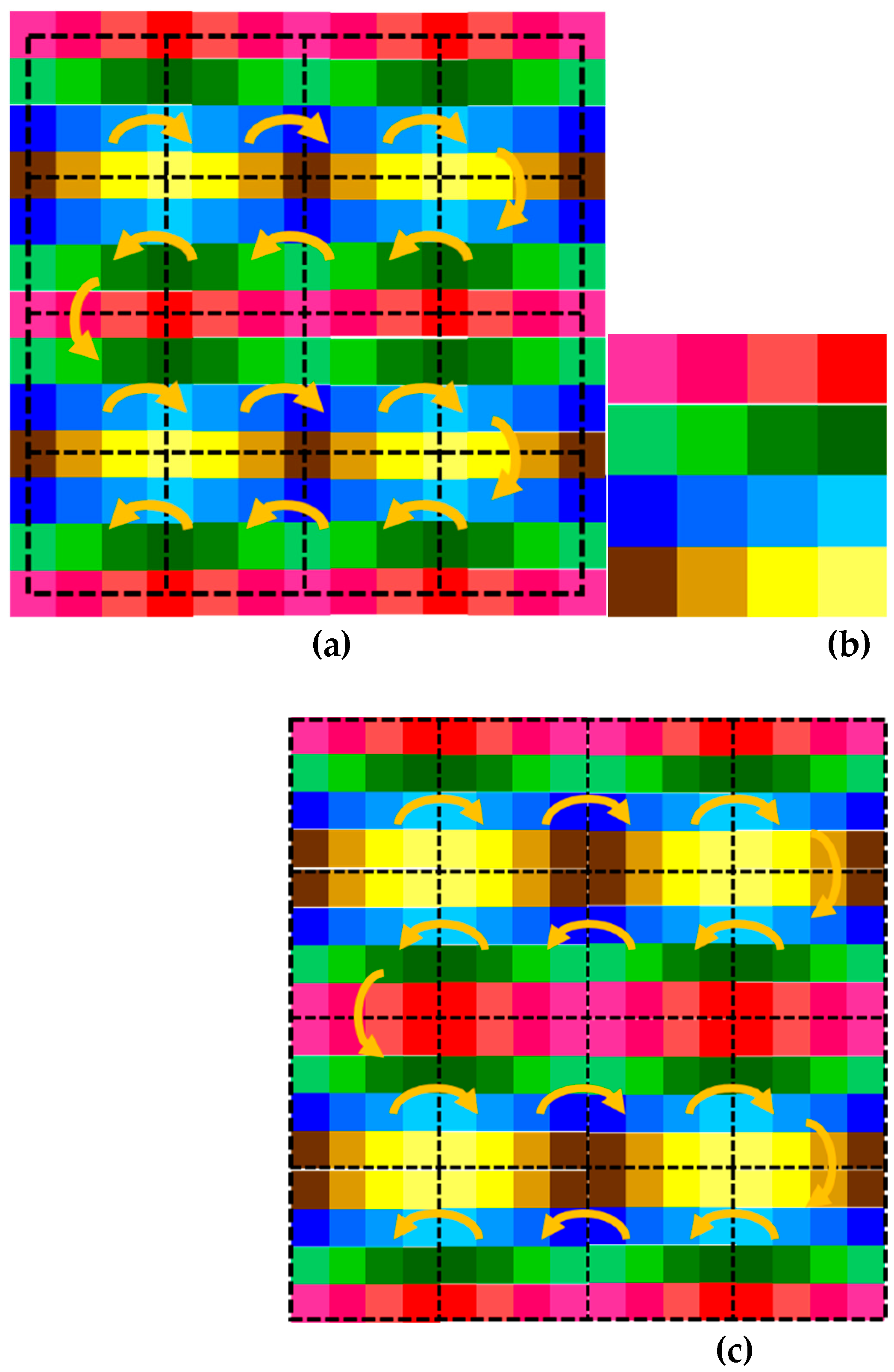
Similarly, scaling SPBOCNN can be accomplished by leveraging the memory of smart pixels at the input and output nodes, along with those in the SPLM, for rapid weight updates. The concept of SPBOCNN scaling is illustrated in Figure 6. The scaling direction is transverse, parallel to the plane of the neural network layer. Consider the entire rectangular region shown in Figure 6(a) as the total computation area for a given problem. This region can be divided into smaller dotted rectangular areas, referred to as elementary blocks, each of which can be processed by SPBOCNN hardware at a time, as shown in Figure 6(b).

In this example, the SPBOCNN consists of input and output layers, as depicted in Figure 5(c). The calculation begins in the top-left corner and shifts sequentially to neighboring blocks, following the yellow arrows in Figure 6(a). For each elementary block, SPBOCNN performs convolution operations between the input and output nodes. When moving to the next block, the output is stored in memory, and the kernel, input, and output nodes are updated.

This process enables the system to scan the entire computation area. A key difference between SPBOCNN and SPBONN scaling is that SPBOCNN maintains partial connections between input and output nodes due to the nature of convolution, whereas SPBONN has fully connected nodes. This introduces more complex topological connections for SPBOCNN when transitioning between neighboring regions, as shown in Figure 6(a).

For instance, consider an elementary block consisting of a 4 × 4 array with a kernel size of 3 × 3, as depicted in Figure 6(b). In convolution, input nodes at the boundary of one block affect the output nodes at the boundary of the neighboring block, depending on the kernel size. In this example, the boundary nodes are influenced by neighboring blocks, and as the kernel size increases to 5 × 5, the interference extends to the second row from the boundary. As a result, calculating boundary nodes within a block requires information from the input nodes of the adjacent block.

This necessity is why boundary cells must be preserved when transitioning to the next block. Notably, the boundary cells retain their colors when shifting to neighboring blocks, as indicated by the yellow arrows in Figure 6(a). The consistent color signifies that the same hardware input nodes are used for their calculation. Thus, transitioning between blocks is not a simple translational shift but rather a topological "flipping."

Overall, all elementary blocks share the same color (or hardware input nodes) with neighboring blocks at their boundaries, forming a seamless connection similar to stitching patches. This ensures accurate convolution across blocks. Figure 6(c) illustrates the redrawn computation area with augmented boundaries, which include a copy of the neighboring block's boundary within each hardware block. In this manner, SPBOCNN scaling in the transverse direction can be achieved.

This approach offers a more flexible method for significantly increasing the input node size, depending on the available memory capacity

Figure 6. An example of scaling the SPBOCNN in the direction parallel to the layer using the stitching method and the memory of smart pixels is as follows: (a) The original calculation area is divided into an array of sectors. Each sector, indicated by dotted lines, is processed by the SPBOCNN hardware one at a time, while the yellow arrows indicate the sequence of calculations; (b) A period of the cells or an elementary block, as calculated by SPBOCNN hardware; and (c) The calculation area is redrawn with augmented boundary cells that contain copies of the boundaries of the neighboring sectors, as the SPBOCNN hardware requires information from neighboring sectors for convolution calculations. The yellow arrows indicate the sequence of calculations when the SPBOCNN hardware scans the entire calculation area using the stitching method

Figure 6. An example of scaling the SPBOCNN in the direction parallel to the layer using the stitching method and the memory of smart pixels is as follows: (a) The original calculation area is divided into an array of sectors. Each sector, indicated by dotted lines, is processed by the SPBOCNN hardware one at a time, while the yellow arrows indicate the sequence of calculations; (b) A period of the cells or an elementary block, as calculated by SPBOCNN hardware; and (c) The calculation area is redrawn with augmented boundary cells that contain copies of the boundaries of the neighboring sectors, as the SPBOCNN hardware requires information from neighboring sectors for convolution calculations. The yellow arrows indicate the sequence of calculations when the SPBOCNN hardware scans the entire calculation area using the stitching method

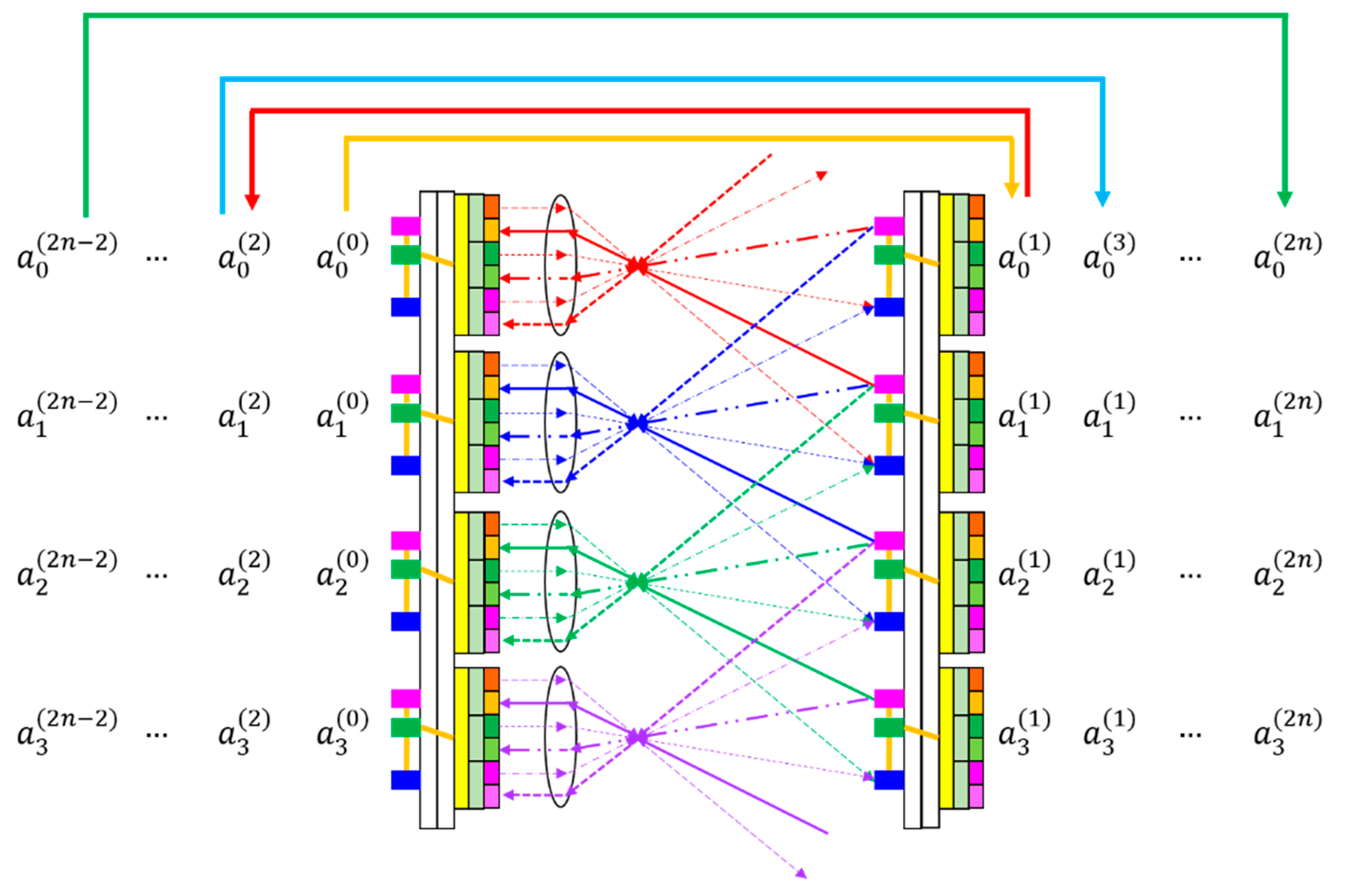
Scaling along the axis perpendicular to the layer plane can be achieved using a two-mirror-like SPBOCNN (TML-SPBOCNN), which serves as a smart pixel adaptation of TMLBONN [19] for convolution. As depicted in Figure 7, data reciprocates between two layers, enabled by the bidirectional nature and rapid reconfigurability of SPBOCNN, attributed to the memory-equipped smart pixels. This TML-SPBOCNN configuration can simulate 2n layers using only 2 physical layers, despite incurring a 2n-fold increase in time delay. For instance, while an 10-layer SPBOCNN achieves 8.3 × 10¹⁵ MAC/s, a 2-layer TML-SPBOCNN can achieve 8.3 × 10¹⁴ MAC/s with a delay that is 10 times longer, while utilizing ten times less space and five times fewer hardware resources. Consequently, TML-SPBOCNN offers a flexible approach to scaling the number of layers through software, which is a critical advantage during the early development phases. Its architecture demands significantly less hardware while emulating any number of layers, contingent on the memory capacity of the smart pixels. Comparatively, replacing the SPLM in TML-SPBOCNN with an SLM reduces parallel throughput by at least 10,000 times, resulting in just 8.3 × 10¹⁰ MAC/s. Hence, the advantages of using the SPLM in TML-SPBOCNN are evident.

Figure 7. An illustration of a TML-SPBOCNN: Data moves reciprocally between the two layers, following the sequence outlined by the arrows above the diagram, simulating the functionality of a multilayer neural network

Figure 7. An illustration of a TML-SPBOCNN: Data moves reciprocally between the two layers, following the sequence outlined by the arrows above the diagram, simulating the functionality of a multilayer neural network

An intriguing application of TML-SPBOCNN is solving partial differential equations (PDEs). Many fundamental physical equations, such as the Poisson equation for gravity, Maxwell's equations, the Schrödinger equation, and others, are expressed as PDEs. These equations depend on local interactions between neighboring cells when the computational domain is divided into discrete cells. For instance, the Laplace equation is shown in equation (1), while its corresponding difference equation is presented in equation (2), where i, j, and k represent the indices of 3-dimensional rectangular cells. According to equation (2), the value of a particular cell is calculated as the average of its nearest neighboring cells. In the relaxation method [23], the function value at a specific position at time step t+1 is computed using the neighboring values from time step t. With continued iterations, the value of each cell converges to the steady-state solution.

$${\nabla }^2\phi =0$$

(1)

$${\phi }_{t+1}\left(i,j,k\right)={\displaystyle \frac{1}{6}}\left[\begin{array}{c}{\phi }_t\left(i-1,j,k\right)+{\phi }_t\left(i+1,j,k\right)+{\phi }_t\left(i,j-1,k\right)+{\phi }_t\left(i,j+1,k\right)\\ +{\phi }_t\left(i,j,k-1\right)+{\phi }_t\left(i,j,k+1\right)\end{array}\right]$$

(2)

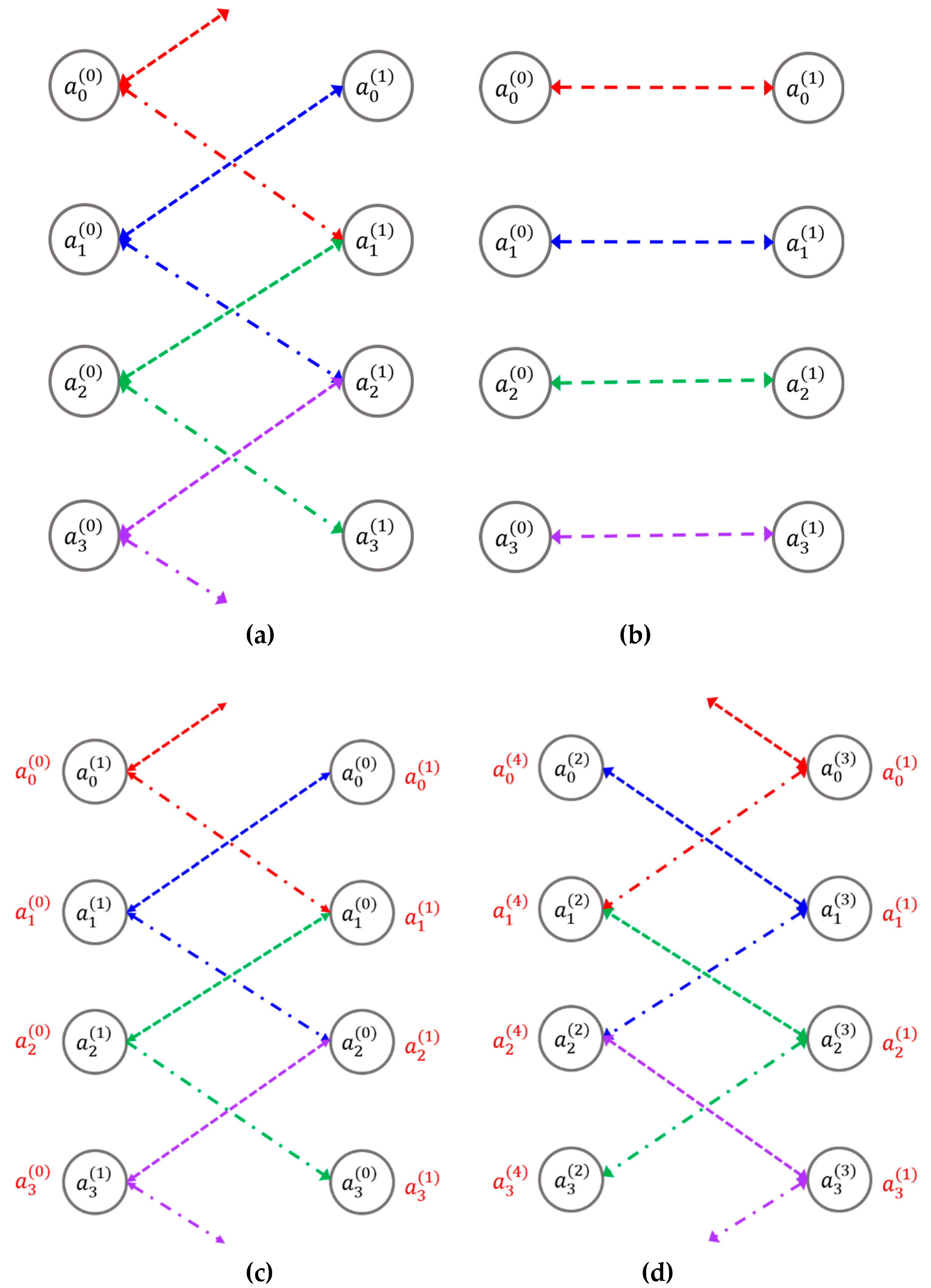
In general, these local interactions can be represented by the convolutions of a neural network. The steps performed by TML-SPBOCNN are illustrated in Figure 8. First, the convolution of the zeroth-layer and first-layer nodes is calculated and stored in the nodes on the opposite side, with data transfer occurring simultaneously in both directions using TML-SPBOCNN, as shown in Figure 8(a). Second, copies of the zeroth and first layers are exchanged. Third, since the node values of the first layer are stored on the left side and the zeroth-layer values on the right during the second step, the convolution of the first layer on the left and the zeroth layer on the right is added to the previously stored values (indicated in red) on the opposite side. Fourth, the convolution of the second-layer and third-layer nodes is computed and stored in the layer on the opposite side, with data transfer occurring simultaneously in both directions. The convolution of the second layer is added to both the stored first-layer value (indicated in red) and the third-layer value. Similarly, the convolution of the third layer is added to the second-layer value and stored for the fourth-layer value (indicated in red). In this manner, the nodes in the first layer collect values from their neighbors in three dimensions, completing the local interactions for the first layer. For the remaining steps, the calculations repeat those shown in Figure 8a–c. The step shown in Figure 8(d) represents the first step of the second cycle.

Figure 8. An example of applying the TML-SPBOCNN to a partial differential equation (PDE) solving problem: (a) The convolution of the zeroth-layer and first-layer nodes is calculated and stored in the nodes on the opposite side, with data transfer occurring simultaneously in both directions; (b) Copies of the zeroth and first layers are exchanged; (c) The convolution of the first layer on the left and the zeroth layer on the right is added to the previously stored values (indicated in red) on the opposite side; (d) The convolution of the second-layer and third-layer nodes is calculated and stored in the layer on the opposite side, with data transfer occurring simultaneously in both directions. The convolution of the second layer is added to both the stored first-layer value (indicated in red) and the third-layer value. Likewise, the convolution of the third layer is added to the second-layer value and stored for the fourth-layer value (indicated in red). In this manner, the nodes in the first layer collect values from their neighbors in three dimensions, completing the local interactions required for PDE solving.

Figure 8. An example of applying the TML-SPBOCNN to a partial differential equation (PDE) solving problem: (a) The convolution of the zeroth-layer and first-layer nodes is calculated and stored in the nodes on the opposite side, with data transfer occurring simultaneously in both directions; (b) Copies of the zeroth and first layers are exchanged; (c) The convolution of the first layer on the left and the zeroth layer on the right is added to the previously stored values (indicated in red) on the opposite side; (d) The convolution of the second-layer and third-layer nodes is calculated and stored in the layer on the opposite side, with data transfer occurring simultaneously in both directions. The convolution of the second layer is added to both the stored first-layer value (indicated in red) and the third-layer value. Likewise, the convolution of the third layer is added to the second-layer value and stored for the fourth-layer value (indicated in red). In this manner, the nodes in the first layer collect values from their neighbors in three dimensions, completing the local interactions required for PDE solving.

5. Conclusions

SPOCNN was proposed to significantly improve the refresh rate of kernels in SOCNN by replacing the SLM with SPLM. It inherits the advantages of SOCNN—such as unlimited input node size, cascadability, and direct kernel representation—unlike a 4f correlator system. Additionally, the fast updating capability and memory of SPLM in SPOCNN enable numerous applications that require real-time updates without significant delay, such as convolution with multiple sets of kernels and difference mode.

SPOCNN was further simplified using electrical fan-out, allowing for the use of a single projection lens instead of three. This eliminates the optical alignment burden and reduces hardware fabrication costs.

SPOCNN evolved into SPBOCNN by adopting the bidirectional architecture concept of BONN. This SPBOCNN was then simplified further into a single lens-array optical system, replacing the three-lens-array optics, by utilizing electric fan-in and fan-out in the SPLMs.

The parallel throughput of SPBOCNN is proportional to the pixel count of the SPLM. For instance, with an SPLM resolution of 3840 × 2160, approximately 8.3 × 10⁶ connections are achieved, enabling 8.3 × 10⁶ MAC operations per cycle. Assuming electronic processing is the primary source of delay—around 10 ns—this system can achieve a computational throughput of 8.3 × 10¹⁴ MAC/s. In comparison, replacing the SPLM in SPBOCNN with an SLM reduces parallel throughput by at least 10,000 times, resulting in only 8.3 × 10¹⁰ MAC/s. Therefore, the advantages of using SPLM in SPBOCNN are clear.

The bidirectional functionality enables SPBOCNN to evolve into TML-SPBOCNN, facilitating data flow between two layers. The TML-SPBOCNN architecture can simulate 2n layers using just 2 physical layers, with a 2n-fold increase in time delay. For example, while an 10-layer SPBOCNN achieves a throughput of 8.3 × 10¹⁵ MAC/s, a 2-layer TML-SPBOCNN can achieve 8.3 × 10¹⁴ MAC/s while requiring ten times less space and five times fewer hardware resources. In this way, TML-SPBOCNN scales in the direction perpendicular to the layers.

Scaling of SPBOCNN is possible in the direction parallel to the layers. Notably, the elementary calculation block includes copies of neighboring cell values at the boundaries, allowing information to be gathered for convolution when transitioning between blocks.

Finally, TML-SPBOCNN was demonstrated to solve partial differential equations (PDEs) in physics. Since PDEs are based on local interactions between neighboring cells in three dimensions, they can be represented by a sequence of convolutions.

In this study, we propose SPOCNN and related architectures along with performance analysis. Due to the numerous advantages outlined, SPOCNN is expected to play a significant role in the future development of versatile convolutional neural network applications.

References

- Hinton, G.; Deng, L.; Yu, D.; Dahl, G.E.; Mohamed, A.R.; Jaitly, N.; Senior, A.; Vanhoucke, V.; Nguyen, P.; Sainath, T.N.; Kingsbury, B. Deep neural networks for acoustic modeling in speech recognition: The shared views of four research groups IEEE Signal processing magazine. 2012; 29, 82–97. [Google Scholar]
- LeCun, Y.; Bengio, Y.; Hinton, G. Deep learning. Nature 2015, 521, 436–444. [Google Scholar] [CrossRef] [PubMed]
- Lecun, L.; Bottou, L.; Bengio, Y.; Haffner, P. Gradient-based learning applied to document recognition Proceedings of the IEEE. 1998; 86, 2278–2324. [Google Scholar]
- Chetlur, S.; Woolley, C.; Vandermersch, P.; Cohen, J.; Tran, J.; Catanzaro, B.; Shelhamer, E. cuDNN: efficient primitives for deep learning. arXiv, 2014; arXiv:1410.0759v3. [Google Scholar]
- Colburn, S.; Chu, Y.; Shilzerman, E.; Majumdar, A. Optical frontend for a convolutional neural network. Applied optics 2019, 58, 3179–3186. [Google Scholar] [CrossRef] [PubMed]
- Chang, J.; Sitzmann, V.; Dun, X.; Heidrich, W.; Wetzstein, G. Hybrid optical-electronic convolutional neural networks with optimized diffractive optics for image classification. Scientific reports, 2018; 8, 12324. [Google Scholar]
- Lin, X.; Rivenson, Y.; Yardimci, N.T.; Veli, M.; Luo, Y.; Jarrahi, M.; Ozcan, A. All-optical machine learning using diffractive deep neural networks. Science, 2018; 361, 1004–1008. [Google Scholar]
- Sui, X.; Wu, Q.; Liu, J.; Chen, Q.; Gu, G. A review of optical neural networks. IEEE Access, 2020; 8, 70773–70783. [Google Scholar]
- Goodman, J.W. Introduction to Fourier optics. Roberts and Company publishers. 2005. [Google Scholar]
- Cox, M.A.; Cheng, L.; Forbes, A. Digital micro-mirror devices for laser beam shaping, Proc. SPIE 11043, Fifth Conference on Sensors, MEMS, and Electro-Optic Systems. 110430Y (2019).
- Mihara, K.; Hanatani, K.; Ishida, T.; Komaki, K.; Takayama, R. High Driving Frequency (> 54 kHz) and Wide Scanning An-gle (> 100 Degrees) MEMS Mirror Applying Secondary Resonance For 2K Resolution AR/MR Glasses. 2022 IEEE 35th Inter-national Conference on Micro Electro Mechanical Systems Conference (MEMS), 477-482 (2022).
- Ju, Y.G. Scalable Optical Convolutional Neural Networks Based on Free-Space Optics Using Lens Arrays and a Spatial Light Modulator. Journal of Imaging 2023, 9, p241. [Google Scholar] [CrossRef] [PubMed]
- Ju, Y.G. A scalable optical computer based on free-space optics using lens arrays and a spatial light modulator. Optical and Quantum Electronics 2023, 55, 1–21. [Google Scholar] [CrossRef]
- Arecchi, A.V.; Messadi, T.; Koshel, R.J. Field Guide to Illumination (SPIE Field Guides vol FG11), SPIE Press, Bellingham, p. 59 (2007).
- Greivenkamp, J.E. Field Guide to Geometrical Optics (SPIE Field Guides Vol. FG01), p.58, SPIE press, Bellingham, p. 28, 73 (2004).
- Seitz, P. Smart Pixels, PROCEEDINGS EDMO 2001 / VIENNA, 229-234 (2001).
- Hinton, H.S. , Progress in the smart pixel technologies. IEEE journal of selected topics in quantum electronics 1996, 2, 14–23. [Google Scholar] [CrossRef]
- Ju, Y.-G. Rapid-Reconfigurable and Flexible Optical Neural Network Based on Free-Space Optics Using Lens Arrays and a Smart Pixel Light Modulator. Preprints 2024, 2024082095. [Google Scholar] [CrossRef]
- Ju, Y.G. Bidirectional Optical Neural Networks Based on Free-Space Optics Using Lens Arrays and Spatial Light Modulator. Micromachines 2024, 15, 701. [Google Scholar] [CrossRef] [PubMed]
- Feng, M.; Wu, C. -H. ; Holonyak N. Oxide-Confined VCSELs for High-Speed Optical Interconnects, IEEE Journal of Quantum Electronics, 2018, 54, 3, pp. 1–15. [Google Scholar]
- James Singh, K.; Huang, Y.M.; Ahmed, T. , Liu; A.C., Huang Chen, S.W.; Liou, F.J.; Wu, T.; Lin, C.C.; Chow, C.W.; Lin, G.R.; Kuo, H.C. Micro-LED as a promising candidate for high-speed visible light communication. Applied Sciences 2020, 10, 7384. [Google Scholar] [CrossRef]
- Glaser, I. Lenslet array processors. Applied Optics, 1982; 21, 1271–1280. [Google Scholar]
- https://en.wikipedia.org/wiki/Relaxation_(iterative_method).
Disclaimer/Publisher’s Note: The statements, opinions and data contained in all publications are solely those of the individual author(s) and contributor(s) and not of MDPI and/or the editor(s). MDPI and/or the editor(s) disclaim responsibility for any injury to people or property resulting from any ideas, methods, instructions or products referred to in the content. |
© 2025 by the author. Licensee MDPI, Basel, Switzerland. This article is an open access article distributed under the terms and conditions of the Creative Commons Attribution (CC BY) license (https://creativecommons.org/licenses/by/4.0/).
Copyright: This open access article is published under a Creative Commons CC BY 4.0 license, which permit the free download, distribution, and reuse, provided that the author and preprint are cited in any reuse.