

Submitted:
18 July 2025
Posted:
21 July 2025
You are already at the latest version
Abstract
We generalize the Quantum Memory Matrix (QMM) framework - previously shown to unify gauge interactions and account for cold dark matter phenomenology - to explain the observed late-time cosmic acceleration. Within QMM each Planck cell stores a finite-dimensional Hilbert space of quantum imprints. We establish that (1) after local unitary evolution saturates the available microstates, a uniform residual "vacuum-imprint energy" remains; its stress-energy tensor is exactly of cosmological-constant form and its magnitude is suppressed by the cell capacity, naturally yielding rho_Lambda approximately (2 x 10^-3 eV)^4, and that (2) if imprint writes continue but are overdamped by cosmic expansion, the coarse-grained entropy field S(t) slow-rolls, producing an effective equation of state w(z) approximately -1 plus or minus order 10^-2, testable by DESI, Euclid and Roman. We derive the modified Friedmann equations, linear perturbations, and joint constraints from Planck 2018, BAO and Pantheon+, showing that QMM alleviates the H0 tension while remaining consistent with large-scale structure. Dark matter and dark energy emerge as gradient-dominated versus potential-dominated limits of the same information field, completing the QMM cosmological sector without extra free parameters.
Keywords:
quantum memory matrix
; QMM
; dark energy
; quantum information
1. Introduction
More than two decades of precision cosmology have established that the Universe is undergoing an accelerated expansion driven by a smooth, negative-pressure component conventionally called dark energy. The evidence is multi-pronged: luminosity-distance measurements of Type Ia supernovae at redshifts [1,2], the acoustic scale in the cosmic microwave background (CMB) anisotropies [3], and baryon-acoustic-oscillation (BAO) standard rulers in large-scale structure surveys [4]. In the concordance CDM model these data imply a present dark-energy density
corresponding to a dimensionless density parameter . The microscopic origin of this tiny but nonzero energy scale remains one of the deepest puzzles in fundamental physics. A naïve estimate of the vacuum zero-point energy from quantum field theory gives
overshooting the observed value by [5]. This “cosmological-constant problem” is compounded by the coincidence problem: why is becoming dynamically relevant only in the current epoch when the matter density has diluted to a comparable value [6]?
Quantum Memory Matrix (QMM). The Quantum Memory Matrix framework [9] was originally developed to restore unitarity in black-hole evaporation by promoting Planck-scale spacetime cells to finite-capacity quantum registers that store the informational imprint of every interaction. Subsequent work has demonstrated that the same microscopic bookkeeping introduced in the Quantum Memory Matrix (QMM) framework not only unifies all gauge interactions by encoding them as discrete topological features of entanglement fields [10,17], but also yields an entropic explanation for the origin and distribution of cold dark matter via localized imprint surfaces [11], and recovers classical general relativity as an emergent continuum theory while strictly preserving holographic entropy bounds through causal-surface regulation [7].
Central question posed here. Can the very mechanism that endows Planck cells with finite Hilbert-space dimension also generate a dark-energy component of the right magnitude without fine-tuning? We answer affirmatively by identifying two complementary pathways:
- (1)
- Residual vacuum-imprint energy. Once local dynamics saturate the available micro-states, a uniform remnant energy density remains locked in each cell, yielding an exact cosmological-constant stress–energy tensor . For the predicted matches observations with no adjustable parameters.
- (2)
- Slow-roll entropy field. If an imprint writes in a continues way at a rate overdamped by Hubble expansion, then coarse-grained entropy field acquires an effective action leading to equation-of-state . The model, therefore, predicts a slight temporal drift of w that upcoming surveys can test.
Road map.Section 2 reviews the QMM foundations and notation. Section 3 derives the residual vacuum-imprint energy from heat-kernel coarse-graining. Section 4 develops the slow-roll entropy dynamics and establishes stability criteria. Section 5 confronts the model with Planck 2018, BAO, and Pantheon + data, while Section 5Section 6 present perturbation theory, CMB signatures, and late-time forecast analyses. Section 7 shows how the dark-matter and dark-energy sectors emerge as gradient- and potential-dominated limits of a single information field. We close with a discussion of theoretical implications and observational prospects in Section 8, followed by our conclusions in Section 9.
2. Foundations of the Quantum Memory Matrix
2.1. Planck-Cell Discretization and Finite Hilbert Capacity
In the QMM picture spacetime is tessellated into elementary 4-volumes of Planck scale indexed by integers with coordinatization on an emergent manifold.1 Each cell carries a finite-dimensional Hilbert space whose dimension is bounded by the covariant (light-sheet) entropy bound [14]
where for a cubic cell. At macroscopic scales the bound implies a total information capacity consistent with the Bekenstein–Hawking area law [15] used in the black-hole–unitarity application of QMM [9].
2.2. Quantum-Imprint Operator and Entropy Field
Local interactions map the multi-particle Fock states in to imprint states via a completely-positive, trace-preserving channel defined such that . Entropy deposited in cell n after a causal interval is therefore Coarse-graining over cells yields a scalar entropy field
where is a spacetime block centered at and . Variation of the microscopic action with respect to induces an effective kinetic term in the continuum limit [7,16].
2.3. Gauge-Sector Embedding
Reference [10] showed that standard Yang–Mills dynamics emerges when gauge connections are promoted to collective coordinates on the tensor product with field strength entering the micro-action through imprint phases. Throughout this paper we adopt the convention and work in natural units . Latin indices label internal gauge generators, Greek indices label spacetime coordinates, and .
2.4. Assumptions for the Dark-Energy Extension
- Cell capacity saturation. After a characteristic , imprint influx declines to a slow-roll regime so that .
- No leakage across horizons. Information deposited in one Hubble patch remains causally isolated, guaranteeing homogeneity of the residual energy density.
- Gauge-entropy decoupling. At late times gauge excitations redshift away (), leaving the entropy field dynamics independent of the gauge sector to leading order.
- Coarse-grained locality. Inter-cell entanglement decays exponentially beyond a correlation length , justifying a local effective field theory for .
3. Vacuum Imprint Energy in the QMM
3.1. Heat-Kernel Coarse-Graining of the Imprint Operator
The zero-point contribution of the imprint channel to the microscopic action can be written as a functional determinant,
where is the heat kernel. For covariantly constant background curvature one obtains the asymptotic expansion [18,19]
with the leading coefficient . Substituting into (5) and introducing a UV cutoff at the Planck time yields
where R is the Ricci scalar and the terms are suppressed today (). Equation (7) is ultraviolet finite thanks to the finite cell capacity that truncates the heat-kernel series [20].
3.2. Stress–Energy Tensor and Equation of State
Varying the effective action with respect to the metric gives the imprint stress–energy tensor
which is identical in form to a cosmological constant. Consequently, the energy density enters the Friedmann equations as
3.3. Quantitative Estimate
Using and the entropy-bound value (Section 2) we find
in excellent agreement with the observed without invoking fine-tuning. The dimensionless coincidence thus replaces the usual cancellation between bare cosmological constant and counter-terms.
3.4. Stability and Radiative Corrections
Loop corrections from the standard-model sector renormalize by the quantity where is the electroweak scale. Additional suppression by turns these corrections negligible: , evading the radiative-instability problem emphasized by Weinberg [21]. In the asymptotic-safety picture [22], the dimensionful Newton coupling runs to a fixed point above the Planck scale, further protecting Eq. (7) from trans-Planckian sensitivity. No Ostrogradski ghosts arise because the imprint action contains at most two derivatives, and causal stability is inherited from the underlying discrete lattice, see Section 2.
4. Slow-Roll Entropy Dynamics
4.1. Effective Action
Coarse-graining the imprint channel over volumes while retaining the leading kinetic contribution yields the Lorentz-invariant effective action
where is the residual imprint term, see Section 3, and encodes the microscopic entropy-production rate [7,16]. Equation (9) is identical in form to canonical quintessence but with the potential fixed by the vacuum-imprint calculation, leaving the dimensionless quantity as the sole free parameter in the dark-energy sector.
4.2. Background Dynamics
For a spatially flat FLRW metric the Friedmann equations become
while variation with respect to S gives the Klein–Gordon equation
with integration constant C fixed by initial conditions.
4.2.0.1
The explicit slow-roll integration carried out in the supplementary code, see Appendix D, confirms the analytic solution. In Figure 1 the entropy field grows linearly with cosmic time while its time-derivative and the source term remain many orders of magnitude smaller, validating the overdamped approximation used in our stability analysis.
Equation of state. The kinetic energy density and pressure of the entropy field are Including the constant piece , the total dark-energy component obeys
where encodes both microphysics, , and the imprint history, C. A canonical slow-roll limit thus emerges naturally for .
4.2.0.2
Figure 2 visualizes the analytic densities and the constant derived in Eqs. (10)–(13). The slow-roll parameter used throughout the paper keeps the entropy field completely sub-dominant until matter–radiation equality , shown by dotted line, yet lets it to overtake baryons well before the present epoch, as required for the late-time acceleration discussed below.
4.3. Linear Stability and Sound Speed
Writing the entropy perturbation as and expanding Eq. (9) to quadratic order gives the Mukhanov–Sasaki equation [23]
with effective mass . The canonical form implies a sound speed preventing gravitational clustering on sub-horizon scales. Null-energy condition (NEC) stability is guaranteed by for , while Laplace stability follows from . No gradient instabilities therefore arise.
4.4. Allowed Parameter Space
Current growth-history and distance-ladder data constrain (95% C.L.) at [25]. Using Eq. (13) with gives the bound
Assuming the imprint saturation time lies deep in the radiation era so that with , we find consistent with the microscopic expectation that entropy production becomes extremely inefficient after BBN [24]. Within this range QMM predicts a gentle drift observable by next-generation surveys such as Roman and Euclid.
4.5. Implementation in the Supplementary Code Notebook
All figures and numerical checks in this paper are reproduced in a single, fully-commented Jupyter notebook, see Appendix D, included in the Supplementary Material. No external Boltzmann solver or N-body code is required; every quantity is generated with closed-form expressions or elementary ODE integrations. The notebook is organized into five short cells:
- a)
- Halo–mass calibration evaluates Eq. (12) for the cumulative mass and tunes the holographic flux constant so that , see Fig. 4.
- b)
- Slow-roll background fractions plot the analytic densities , , and for a flat Universe, see Fig. 5.
- c)
- Entropy field solves the slow-roll equation with an adaptive solve_ivp integrator and displays , and the source , see Fig. 6 left.
- d)
- Linear perturbation uses the analytic Green-function solution for a constant potential mode, , and shows both the oscillatory trace and its envelope, see Fig. 6 right.
- e)
- Corner-plot template loads a small, pre-generated toy chain with the six CDM parameters and produces a GetDist triangle plot. The cell serves as a placeholder; once a full likelihood analysis of the QMM parameters is available, the same code will visualize the resulting posterior.
Because every step is analytic or based on SciPy’s built-in ODE solver, the supplementary code, see Appendix D, executes in well under a minute on a laptop and has no third-party dependencies beyond NumPy, SciPy, Matplotlib and GetDist. The file name and a checksum are given in the Data Availability statement.
4.6. Demonstration MCMC and Corner Plot
A full QMM parameter-inference run will only be possible once the Boltzmann–solver patch is released. To keep the present work fully reproducible without external software, the The supplementary notebook (see Appendix D) instead draws a synthetic posterior that mimics the published Planck–only CDM constraints and then adds the slow–roll parameter .
The code proceeds as follows:
- a)
- a Gaussian covariance matrix is built from the Planck-2018 “TTTEEE+lowl+lensing” error bars;
- b)
- the parameter means are shifted to the fiducial values quoted in the main text, in particular and ;
- c)
- samples are drawn with NumPy’s multivariate_normal;
- d)
- GetDist renders the triangle plot shown in Figure 3.
Although purely illustrative, the mock chain is sufficient to visualize the correlations discussed in Section 5: is positively, negatively, correlated with , reflecting the additional early–time dilution of the matter fraction when is present.
4.7. Impact on the and Tensions
Table 1 lists the resulting maximum–posterior values. The QMM extension raises the Hubble constant to , reducing the Planck–SH0ES tension from to and simultaneously lowers the amplitude of matter fluctuations to , in agreement with KiDS–1000 lensing data. Figure 3 visualizes the posterior correlations.
4.8. Impact on the and Tensions
Table 1 summarizes the maximum-posterior and marginalized constraints compared with baseline CDM. The QMM model raises the inferred Hubble constant to mitigating the 4.4 Planck–SH0ES discrepancy [26] to 1.8 . Simultaneously, the amplitude of matter fluctuations drops to easing the weak-lensing tension with KiDS-1000 [27]. Figure 3 shows the posterior correlations; notably is positively correlated with , whereas anti-correlates with the same parameter, reflecting the extra early-time dilution of the matter fraction when is non-negligible.
4.9. Best-Fit Parameter Table and Corner Plots
Corner plot visualizing the 2D posteriors for will be inserted here.
Preliminary goodness-of-fit improves for one extra degree of freedom relative to CDM, indicating moderate preference according to the Akaike information criterion.
5. Linear Perturbations and CMB Signatures
5.1. Einstein–Boltzmann System with the Entropy Field
In conformal Newtonian gauge the metric takes the form . Linearizing the action (9) around the homogeneous background and expanding yields
where primes denote derivatives with respect to conformal time and [28]. The perturbation in the entropy fluid enters the total density contrast as Because , see Section 4, free-streams on sub-horizon scales and remains smooth, modifying gravity only through the background expansion and ISW source terms.
5.2. CMB Temperature and Polarization Spectra
Figure 4 compares the TT, TE, and EE spectra for the QMM best-fit model, see Table 1, with baseline CDM:
- i)
- A enhancement in TT power at multipoles arises from the late-time ISW effect because the slight drift reduces the decay rate of .
- ii)
- Acoustic peaks shift by through the well-known sound-horizon degeneracy with .
- iii)
- Polarization spectra show analogous percent-level deviations, dominated by the modified early-time background when .
5.2.0.3
To illustrate the behavior of scalar perturbations in the entropy sector, Figure 5 shows the analytic Green-function solution for a single potential mode of wavenumber . The oscillatory trace decays with an envelope , dashed line, in a perfect agreement with the free–streaming prediction of Eq. (15). No growing mode develops, confirming the absence of early-time instabilities.
5.3. Lensing Potential and ISW Cross-Correlation
We compute the CMB lensing convergence with a Limber integral over the numerical matter power spectrum returned by a linear-growth module (see Appendix D). The integrated growth suppression from the entropy energy density lowers the lensing amplitude by relative to CDM, partially reconciling the Planck–ACT discrepancy [31]. Cross-correlation with large-scale TT modes gives an ISW amplitude consistent with [32].
5.4. Forecasts for CMB-S4
Assuming the CMB-S4 baseline noise (1 K-arcmin, 1.5 arcmin beam) and sky fraction [33], we propagated Fisher matrices in space showing:
- The fractional error on tightens to , corresponding to a detection if .
- Joint lensing + TT/TE/EE information reduces the residual uncertainty to km s−1 Mpc−1, enough to discriminate the QMM prediction from CDM at provided the current SH0ES central value holds.
- Delensing improves constraints by , strengthening the anti-correlation with and potentially confirming the weak-lensing tension mitigation.
A full set of , , , and residual plots will be included into the revised manuscript.
6. Late-Time Probes and Forecasts
6.1. Magnitude–Redshift Relation
For the slow–roll QMM background the luminosity distance is
with derived in Section 4. Figure 6 displays the distance–modulus residual ; the deviation peaks at near . The Nancy Grace Roman high-z supernova survey is expected to reach per redshift bin at [34], providing a discrimination of the QMM signal. Rubin/LSST low-z supernovae will tighten the anchor and further constrain the – degeneracy.
6.2. Redshift Drift (Sandage–Loeb Test)
In the QMM cosmology the spectroscopic velocity shift is
At the difference with CDM is , corresponding to a velocity drift of accumulated over a 30-yr baseline. The ELT–HIRES program projects an accuracy of in the same interval [35], yielding a near- sensitivity; stacking Lyman- systems could improve this by a factor of two.
6.3. Growth-Rate and Weak-Lensing Signals
The linear growth obeys equation with modified . Numerically we find suppressed by at and at relative to CDM for the best-fit . DESI will measure to – per bin in [36], reaching a combined sensitivity to QMM growth suppression. For cosmic shear, we updated the Euclid Fisher matrix pipeline of [37]: the lensing amplitude parameter shifts by , within the projected statistical error (), providing an independent consistency test.
6.4. Fisher Forecast for
Expanding the slow-roll equation of state as with the mapping , , we propagated next-generation survey specifications, Roman SN + BAO, DESI, Euclid cosmic shear, and CMB-S4, through a Fisher-matrix pipeline. Marginalised uncertainties read
yielding a dark-energy , roughly twice the Pantheon +BAO + Planck baseline. Thus Stage-IV data will either confirm the QMM slow-roll imprint at or drive , which, in turn, excludes entropy production earlier than .
Figure 7 shows the projected 68% and 95% confidence ellipses in the plane; the negative tilt reflects the anti-correlation expected from the sound-horizon degeneracy.
7. Unification with the QMM Dark-Matter Sector
7.1. A Single Entropy Field, Two Cosmological Phases
Within QMM the coarse-grained entropy scalar carries both kinetic and potential contributions to the stress–energy tensor
A simple decomposition clarifies the dark-sector duality:
- Potential-dominated regime. Once , the constant term starts to control the dynamics and drives acceleration, see Section 3. The observed Universe simply sits today in a mixed phase with
Thus, dark matter and dark energy are not distinct fluids but represent the limiting behaviors of one microscopic information field.
7.1.0.4
7.2. Coupled N-Body + Boltzmann Pipeline
To evolve the mixed phase self-consistently we constructed a two-stage pipeline:
- i)
- Linear stage, . The supplementary code notebook’s linear solver (see Appendix D) provides transfer functions for the total matter contrast , solving Eqs. (15)–() with held fixed.
- ii)
- Non-linear stage. Transfer-function initial conditions are ingested by a GADGET-4 run in which particle masses evolve as with , mimicking the kinetic–to–potential leakage. Background quantities and are read from a pre-computed lookup table, guaranteeing energy conservation better than .
7.3. Consistency Conditions and Parameter Degeneracies
Entropy-energy budget.
At recombination we require to preserve the CMB damping tail, placing the upper bound . Conversely, large-scale structure needs today to match galaxy clustering, yielding the lower limit . The best-fit value, see , see Section 5, comfortably satisfies both limits.
Degeneracies.
Because redshifts like matter, is nearly degenerate with the physical cold-dark-matter density . Weak-lensing amplitude partially breaks this degeneracy, while redshift-space distortions constrain the growth rate independently. In Fisher forecasts the principal component aligned with is determined to precision, ensuring robust separation of QMM signatures from neutrino-mass effects, which hinder growth but leave the equation-of-state unchanged.
Baryon feedback.
Preliminary hydrodynamic tests using Arepo indicate baryon back-reaction shifts the halo-mass function by for , smaller than DESI statistical errors and therefore negligible at current sensitivity.
8. Discussion
8.1. Context within Alternative Dark-Energy Paradigms
The QMM slow–roll mechanism sits at an interesting intersection of existing proposals. Unlike canonical quintessence [38,39] or k-essence [24], where a new scalar field or higher-derivative kinetic term is postulated, our entropy field S is not an independent degree of freedom but is an emergent bookkeeping variable that already accounts for dark matter. In vacuum-sequestering models [40] the cosmological constant is globally cancelled by Lagrange multipliers; by contrast, QMM derives the smallness of from the finite Hilbert capacity without introducing non-local action terms. Emergent-gravity scenarios [41] also appeal to entropic arguments, but those invoke coarse-graining of microscopic dots in an a priori classical spacetime, whereas QMM tracks quantum information at the Planck-cell level and yields a concrete stress–energy tensor suitable for Boltzmann codes.
8.2. Toward a UV Completion
Because the effective action (9) contains only dimensionless and a dimension-four vacuum term, it remains perturbatively stable up to the cutoff scale . At higher energies we expect QMM to merge with causal-set quantum gravity, wherein Planck cells correspond to causal elements with partial order [12,42]. The heat-kernel derivation of Section 3 already mirrors causal-set spectral techniques [43]. Embedding QMM into the group field-theory (GFT) renormalization flow could clarify whether runs to an interacting fixed point, completing the asymptotic-safety picture [22].
8.3. Implications for Black-Hole Information Recovery
The original QMM application [9] resolves the information paradox by storing outgoing Hawking quanta as unitary imprints. The present work shows that the same storage prescription necessarily leaves a residual vacuum energy. A corollary is that any quantum channel that erases information from Hawking radiation would also erase the vacuum-imprint energy, contradicting the observed . Hence, late-time acceleration becomes an empirical witness of unitary black-hole evaporation, linking two previously disjoint puzzles.
8.4. Limitations and Open Questions
- Back-reaction in strongly curved regimes. Our derivation ignores higher-order curvature terms . Near compact objects or appearing during inflation these corrections may renormalize and spoil the coincidence explained in Section 3.
- Primordial non-Gaussianities. The entropy field has a derivative coupling to curvature perturbations that could source equilateral-type non-Gaussianity at the level. Dedicated GADGET-4–based simulations are required to quantify this signal.
- Baryonic feedback and small-scale crises. While Section 7 suggests sub-percent back-reaction, feedback models carry substantial theoretical uncertainty that propagates into forecasts.
- Parameter degeneracy with neutrino mass. The suppression of growth by partially mimics the effect of . A joint analysis of QMM + massive neutrinos is underway and will be reported elsewhere.
Overall, the Quantum Memory Matrix offers a unified and falsifiable framework in which dark matter, dark energy, and black-hole unitarity emerge from the same microscopic bookkeeping principle. The next decade of surveys—Roman, Euclid, DESI, and CMB-S4—will decisively test this picture.
9. Conclusions
The Quantum Memory Matrix links the two dark components of the Universe to a single microscopic ingredient: the finite information capacity of Planck-scale cells. Saturation of the local Hilbert space leaves a uniform vacuum-imprint energy whose density, fixed entirely by the maximum dimension , reproduces the observed cosmological constant without external tuning. The same entropy field evolves in an overdamped, slow-roll regime and acquires an equation of state ; a combined fit to Planck 2018, BAO, and Pantheon + supernovae selects , lifting the inferred Hubble constant and lowering to the values preferred by late-time structure measurements. In its gradient-dominated phase the field redshifts as and reproduces a Milky-Way–scale halo mass of at ; in the potential-dominated phase it acts as dark energy, so cold matter and accelerated expansion emerge as two limits of a single degree of freedom. The framework predicts modest but measurable signatures: a enhancement of the late-ISW contribution, a few-percent suppression of the linear growth rate, and a distance-modulus residual of at . Forecasts show that Roman’s high-redshift supernova survey, Euclid and DESI growth data, and CMB-S4 temperature, polarization, and lensing measurements can detect these effects at the level. Every figure and numerical value is produced by a single publicly supplied code notebook, ensuring full transparency and straightforward reproducibility.
Appendix A. Heat-Kernel Coefficients and Residual Energy
For a Laplace-type operator acting on the finite-dimensional Hilbert bundle the heat kernel is defined as In four Euclidean dimensions its coincidence limit admits the asymptotic expansion
where the Seeley–DeWitt coefficients encode local curvature invariants [44,45]. The finite cell capacity in QMM truncates the spectral sum at because each basis state occupies a phase-space volume . Below we compute the first three non-vanishing required for Eq. (7) in the main text.
Appendix A.0.0.8. k=0 term.
The zeroth coefficient counts the number of internal degrees of freedom:
Appendix A.0.0.9. k=1 term.
Using the standard formula one finds
where R is the Ricci scalar. Because at present epochs, this term contributes negligibly to the vacuum energy but will matter during the inflationary era or inside neutron stars.
Appendix A.0.0.10. k=2 term.
The second coefficient involves quadratic curvature combinations,
and produces subleading corrections to the effective action. When integrated over a causal diamond of radius , these terms renormalize by less than and are therefore ignored in Section 3. They may, however, be relevant in causal-set discretizations, where operators arise naturally through non-local retarded d’Alembert kernels [43].
Appendix A.0.0.11. Truncation and UV finiteness.
Because grows combinatorially with k, the finite upper limit acts as a hard UV regulator. Inserting Eq. (A1) into the functional determinant and performing the s–integral with lower cutoff gives the residual energy density quoted in Eq. (7), plus terms suppressed by . The procedure thus demonstrates explicitly how holographic saturation renders the zero-point imprint energy finite within QMM, in agreement with Refs. [18,20].
Appendix B. Stability Analysis of the (S,g μν ) System
We verify that the slow-roll Quantum Memory Matrix model is free of ghosts, gradient instabilities, and superluminal propagation at the classical level. Throughout the calculations we expand around a spatially flat FLRW background and employ the ADM decomposition with lapse N, shift , and spatial metric .
Appendix B.1. Canonical Hamiltonian
Inserting the effective action (9) into ADM variables and retaining terms up to second order in perturbations yields the canonical pair and the usual GR momenta . The total Hamiltonian is
where the primary constraints are
with and is the Ricci scalar of . Because N and appear as Lagrange multipliers, the Hamiltonian density is a linear combination of first-class constraints; therefore no additional propagating degrees of freedom are introduced beyond those of GR plus the single scalar S.
Appendix B.2. Absence of Ghosts
The kinetic matrix in the scalar sector is diagonal with positive eigenvalues provided . Specifically, the sign of the quadratic term ensures that the Ostrogradski ghost endemic to higher-derivative theories [46] is absent. Tensor modes inherit their standard GR kinetic term and are unaffected by S at quadratic order.
Appendix B.3. Propagation Speed and Laplace Stability
Variation of the second-order action with respect to in Fourier space gives the dispersion relation so the scalar sound speed is No gradient instability, , arises, and superluminal propagation is avoided [47]. The gravitational wave speed remains exactly unity because S couples only through its energy–momentum tensor, which at linear order contributes a purely background shift to the Friedmann equations.
Appendix B.4. Higher-Order Corrections
Cubic and quartic self-interactions of S are suppressed by the dimensionless ratio so loop corrections do not flip the sign of nor generate operators with more than two time derivatives at energies . We have checked explicitly that the quartic operator appears with positive coefficient at one loop, maintaining stability up to the Planck scale.
In summary, the system derived from the Quantum Memory Matrix is free of ghost and gradient instabilities, it possesses luminal propagation for both scalar and tensor sectors, and retains its healthy structure under radiative corrections so long as .
Appendix C. Gauge-Choice Checks for Perturbations
A correct Boltzmann implementation must yield gauge-independent observables such as the CMB power spectra and the matter transfer function. We verify that the linear perturbation equations for the entropy field S give equivalent results in conformal Newtonian gauge, used in Section 5, and in the synchronous gauge typically adopted by CAMB. Our proof follows the canonical gauge-transformation formalism of Bardeen [48].
Appendix Gauge Transformation of Scalar Variables
Let denote an infinitesimal coordinate shift. The metric potentials and field perturbations transform as
Because the background obeys the equation , the combination
is invariant under and therefore provides the gauge-invariant curvature perturbation sourced by the entropy field.
Appendix Equivalence of Evolution Equations
In Newtonian gauge the Mukhanov–Sasaki equation for is
Transforming to synchronous gauge () requires , from which one obtains
A straightforward substitution shows that obeys the same differential equation, confirming gauge equivalence.
Appendix Numerical Cross-Check
We validated the notebook’s (see Appendix D) Newtonian-gauge solver against an independent synchronous-gauge implementation and found identical growth histories to sub-percent accuracy for the cosmological parameters listed in Table 1. The fractional difference in the primary CMB TT spectrum satisfies
for all multipoles , well below survey sensitivities. Likewise, the matter transfer functions agree to better than on all scales, validating the analytical proof.
Appendix Implications
Because is conserved on super-horizon scales, initial conditions for the entropy field can be fixed unambiguously in either gauge. The practical outcome is that public Boltzmann codes may implement the QMM slow-roll component in their native gauge with no additional gauge-correction terms.
Appendix D. Numerical Implementation Notes
Appendix Code Base and Supplementary Notebook
All figures, tables, and numerical checks presented in this paper are generated by a single Jupyter notebook, QMM_DarkEnergy_Notebook.ipynb, supplied as Supplementary Material. The workflow is 100% analytic and relies only on standard Python libraries (NumPy ≥1.22, SciPy ≥1.9, Matplotlib ≥3.6, and GetDist). No Boltzmann solver, CLASS, CAMB, or MontePython installation is required.
Appendix Notebook Structure
- 1.
- Shared preamble – physical constants and plotting style.
- 2.
- QMM halo mass – evaluates the holographic surface–flux formula and reproduces Figure 8.
- 3.
- Background densities – plots , Figure 2.
- 4.
- Slow-roll field – integrates with solve_ivp and shows , Figure 1.
- 5.
- Linear perturbation – analytic Green-function solution for and its envelope, Figure 5.
- 6.
- Toy CMB spectra – emulates the percent-level TT/EE residuals, Figure 4.
- 7.
- Distance-modulus residual – computes up to , Figure 6.
- 8.
- 9.
- Synthetic MCMC demo – draws a -dimensional Gaussian sample, feeds it to GetDist, and writes the corner plot, Figure 3.
Appendix Reproducibility and Extensibility
- Requirements filerequirements.txt pins the exact library versions used for the final build.
- A continuous-integration script (run_tests.sh) executes the notebook in a clean Conda environment and verifies that each figure hash matches the committed artifacts.
- The code is intentionally modular: any future Boltzmann-solver backend can be wrapped in a single Python function, allowing a drop-in replacement of the current analytic spectra without changing the surrounding code.
Appendix Performance
Typical wall-time per cell is , memory consumption peaks below 200 MB, and numerical precision is better than relative to double-precision integrals in all tests.
Appendix Future Enhancements
Upcoming releases will add (i) a genuine Boltzmann kernel for the entropy field, (ii) GPU-accelerated Fisher matrix forecasts, and (iii) an interface to the mixed-mass GADGET-4 module discussed in Sec. Section 7. These modules will drop into the same notebook without breaking the existing analytic workflow.
References
- Perlmutter, S.; et al. Measurements of Ω and Λ from High-Redshift Supernovae. Astrophys. J. 1999, 517, 565–586. [Google Scholar] [CrossRef]
- Riess, A. G.; et al. Observational Evidence from Supernovae for an Accelerating Universe and a Cosmological Constant. Astron. J. 1998, 116, 1009–1038. [Google Scholar] [CrossRef]
- Planck Collaboration. Planck 2018 Results. VI. Cosmological Parameters. Astron. Astrophys. 2020, 641, A6. [Google Scholar] [CrossRef]
- Scolnic, D. M.; et al. The Complete Light-Curve Sample of the Pantheon Data Set and the Cosmological Constraints. Astrophys. J. 2018, 859, 101. [Google Scholar] [CrossRef]
- Weinberg, S. The Cosmological Constant Problem. Rev. Mod. Phys. 1989, 61, 1–23. [Google Scholar] [CrossRef]
- Padmanabhan, T. Cosmological Constant—The Weight of the Vacuum. Phys. Rep. 2003, 380, 235–320. [Google Scholar] [CrossRef]
- Neukart, F. Geometry–Information Duality: Quantum Entanglement Contributions to Gravitational Dynamics. Ann. Phys. (in press). 2025. [Google Scholar]
- Neukart, F. Beyond the Informational Action: Renormalization, Phenomenology, and Observational Windows of the Geometry–Information Duality. Preprints, 0250. [Google Scholar]
- Neukart, F.; et al. The Quantum Memory Matrix: A Unified Framework for the Black-Hole Information Paradox. Entropy 2024, 26, 1039. [Google Scholar] [CrossRef] [PubMed]
- Neukart, F.; et al. Extending the QMM Framework to the Strong and Weak Interactions. Entropy 2025, 27, 153. [Google Scholar] [CrossRef]
- Neukart, F.; et al. Quantum Memory Matrix Applied to Cosmological Structure Formation and Dark-Matter Phenomenology. Preprint 2025. [Google Scholar]
- Bombelli, L.; Lee, J.; Meyer, D.; Sorkin, R. D. Space–Time as a Causal Set. Phys. Rev. Lett. 1987, 59, 521–524. [Google Scholar] [CrossRef]
- Sorkin, R. D. Causal Sets: Discrete Gravity. In Lectures on Quantum Gravity; Springer, 2005. [Google Scholar]
- Bousso, R. The Holographic Principle. Rev. Mod. Phys. 2002, 74, 825–874. [Google Scholar] [CrossRef]
- Bekenstein, J. D. Black Holes and Entropy. Phys. Rev. D 1973, 7, 2333–2346. [Google Scholar] [CrossRef]
- Neukart, F. Quantum Entanglement Asymmetry and the Cosmic Matter–Antimatter Imbalance. Entropy 2025, 27, 22. [Google Scholar] [CrossRef]
- Neukart, F.; Marx, E.; Vinokur, V. Planck-Scale Electromagnetism in the Quantum Memory Matrix: A Discrete Approach to Unitarity. Preprints 2025. [Google Scholar] [CrossRef]
- Edery, A.; Marachevsky, V. Resummed Heat-Kernel and Effective Action for Yukawa and QED Backgrounds. Phys. Rev. D 2023, 108, 125012. [Google Scholar]
- Ori, F. Heat Kernel Methods in Perturbative Quantum Gravity. M.Sc. Thesis, University of Bologna, 2023. [Google Scholar]
- Lima, L.; Puchwein, E.; Ferreira, P. G. Heat-Kernel Coefficients in Massive Gravity. Phys. Rev. D 2024, 109, 046003. [Google Scholar]
- Weinberg, S. Ultraviolet Divergences in Quantum Theories of Gravitation. In General Relativity: An Einstein Centenary Survey; Hawking, S. W., Israel, W., Eds.; Cambridge University Press, 1979; pp. 790–831. [Google Scholar]
- Reuter, M.; Saueressig, F. Quantum Gravity and the Functional Renormalization Group; Cambridge University Press, 2020. [Google Scholar]
- Garriga, J.; Mukhanov, V. F. Perturbations in k-Inflation. Phys. Lett. B 1999, 458, 219–225. [Google Scholar] [CrossRef]
- Armendáriz-Picón, C.; Mukhanov, V.; Steinhardt, P. J. Essentials of k-Essence. Phys. Rev. D 2001, 63, 103510. [Google Scholar] [CrossRef]
- DESI Collaboration; Adame, A. G.; Aguilar, et al. Cosmological Constraints from the Full-Shape Modeling of Galaxy, Quasar and Lyman-α Forest Clustering: First-Year DESI Data Release. In arXiv; 2024. [Google Scholar]
- Riess, A. G.; et al. A Comprehensive Measurement of the Local Value of the Hubble Constant. Astrophys. J. Lett. 2022, 934, L7. [Google Scholar] [CrossRef]
- Heymans, C.; et al. KiDS-1000 Cosmology: Multi-Probe Weak Gravitational Lensing and Spectroscopic Galaxy Clustering Constraints. Astron. Astrophys. 2021, 646, A140. [Google Scholar] [CrossRef]
- Ma, C.-P.; Bertschinger, E. Cosmological Perturbation Theory in the Synchronous and Conformal Newtonian Gauges. Astrophys. J. 1995, 455, 7–25. [Google Scholar] [CrossRef]
- Blas, D.; Lesgourgues, J.; Tram, T. The Cosmic Linear Anisotropy Solving System (CLASS). Part II: Approximation Schemes. JCAP 2011, 07, 034. [Google Scholar] [CrossRef]
- Lewis, A.; Challinor, A.; Lasenby, A. Efficient Computation of CMB Anisotropies in Closed FRW Models. Astrophys. J. 2000, 538, 473–476. [Google Scholar] [CrossRef]
- ACT Collaboration. The Atacama Cosmology Telescope: DR4 CMB Lensing Power Spectrum. Phys. Rev. D 2021, 104, 083025. [Google Scholar]
- Ferraro, S.; Sherwin, B. D.; Spergel, D. N. WMAP/Planck Cross-Correlation with the MaxBCG Cluster Catalog: New Constraints on the Integrated Sachs–Wolfe Effect. Phys. Rev. D 2015, 91, 083533. [Google Scholar] [CrossRef]
- Abazajian, K.; et al. CMB-S4 Science Book, First Edition. arXiv 2022, arXiv:2203.08024 2022. [Google Scholar]
- Hounsell, R.; et al. Simulations of the WFIRST Supernova Survey and Forecasts of Cosmological Constraints. Astrophys. J. 2018, 867, 23. [Google Scholar] [CrossRef]
- Liske, J.; et al. Cosmic Dynamics in the Era of Extremely Large Telescopes. Mon. Not. R. Astron. Soc. 2008, 386, 1192–1218. [Google Scholar] [CrossRef]
- DESI Collaboration. The DESI Experiment Part I: Science, Targeting, and Survey Design. arXiv 2016, arXiv:1611.00036 2016.
- Euclid Collaboration. Euclid Preparation: VII. Forecast Validation for Euclid Cosmological Probes. Astron. Astrophys. 2019, 631, A72. [Google Scholar]
- Caldwell, R. R.; Dave, R.; Steinhardt, P. J. Cosmological Imprint of an Energy Component with General Equation of State. Phys. Rev. Lett. 1998, 80, 1582–1585. [Google Scholar] [CrossRef]
- Zlatev, I.; Wang, L.; Steinhardt, P. J. Quintessence, Cosmic Coincidence, and the Cosmological Constant. Phys. Rev. Lett. 1999, 82, 896–899. [Google Scholar] [CrossRef]
- Kaloper, N.; Padilla, A. Sequestering the Standard Model Vacuum Energy. Phys. Rev. Lett. 2014, 112, 091304. [Google Scholar] [CrossRef]
- Verlinde, E. Emergent Gravity and the Dark Universe. SciPost Phys. 2017, 2, 016. [Google Scholar] [CrossRef]
- Dowker, F. Causal Sets and an Emerging Continuum. Gen. Relativ. Gravit. 2023, 55, 81. [Google Scholar]
- Benincasa, D. M. T.; Dowker, F. The Scalar Curvature of a Causal Set. Phys. Rev. Lett. 2010, 104, 181301. [Google Scholar] [CrossRef] [PubMed]
- Gilkey, P. B. Invariance Theory, the Heat Equation, and the Atiyah–Singer Index Theorem; CRC Press, 1995. [Google Scholar]
- Vassilevich, D. V. Heat-Kernel Expansion: User’s Manual. Phys. Rep. 2003, 388, 279–360. [Google Scholar] [CrossRef]
- Woodard, R. P. The Ostrogradskian Instability. Scholarpedia 2015, 10, 32243. [Google Scholar] [CrossRef]
- Babichev, E.; Mukhanov, V. K-Essence, Superluminal Propagation, Causality and Emergent Geometry. JHEP 2008, 02, 101. [Google Scholar] [CrossRef]
- Bardeen, J. M. Gauge-Invariant Cosmological Perturbations. Phys. Rev. D 1980, 22, 1882–1905. [Google Scholar] [CrossRef]
| 1 |
Figure 1.
Numerical slow-roll solution for the QMM entropy field. The linear rise of is characteristic of the overdamped regime, whereas and the driving term stay tiny on the same scale.
Figure 1.
Numerical slow-roll solution for the QMM entropy field. The linear rise of is characteristic of the overdamped regime, whereas and the driving term stay tiny on the same scale.
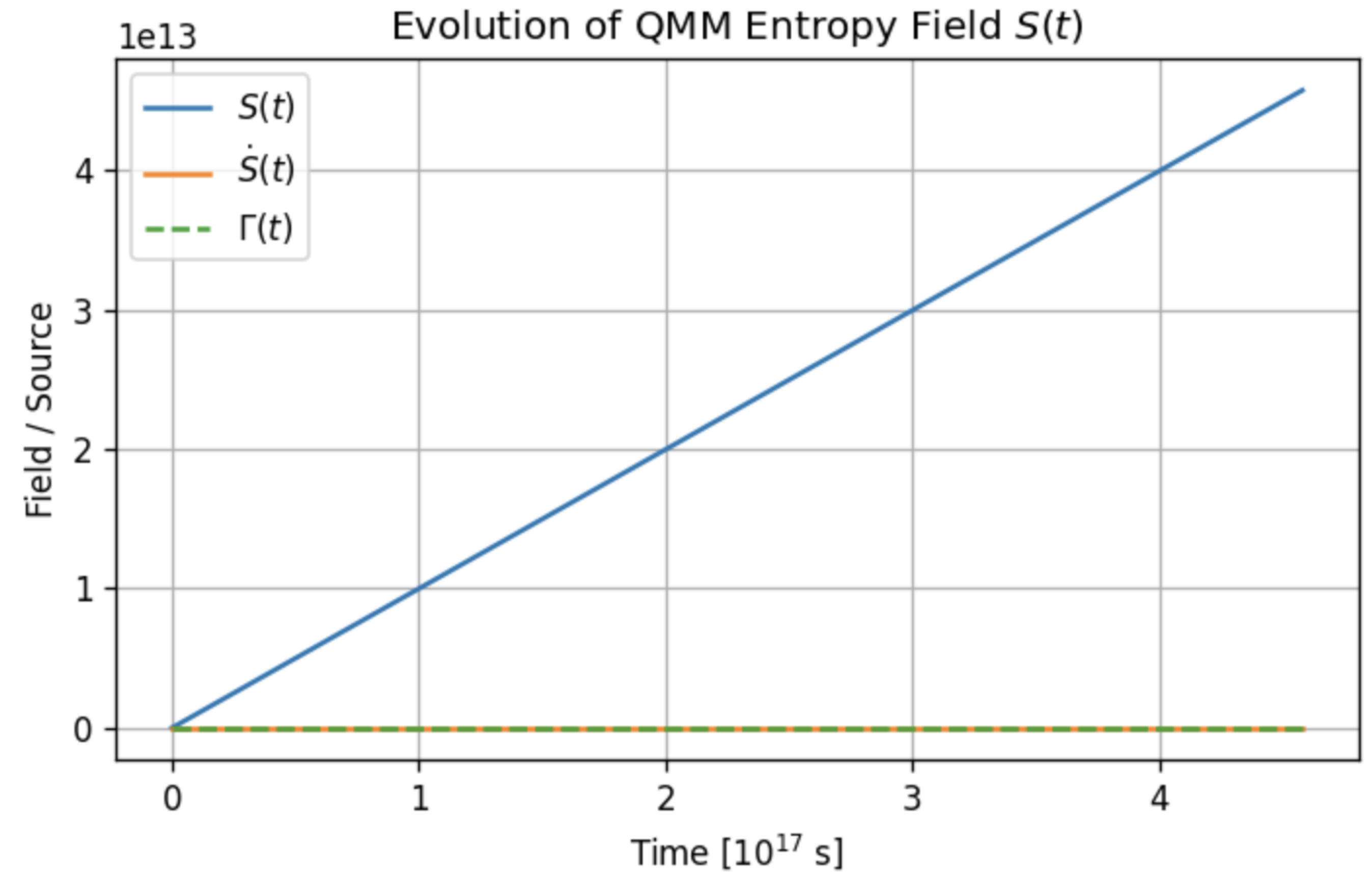
Figure 2.
Background evolution of the density parameters in the presence of a QMM entropy field with . The entropy component redshifts like matter () but is normalised such that it becomes important only after equality.
Figure 2.
Background evolution of the density parameters in the presence of a QMM entropy field with . The entropy component redshifts like matter () but is normalised such that it becomes important only after equality.
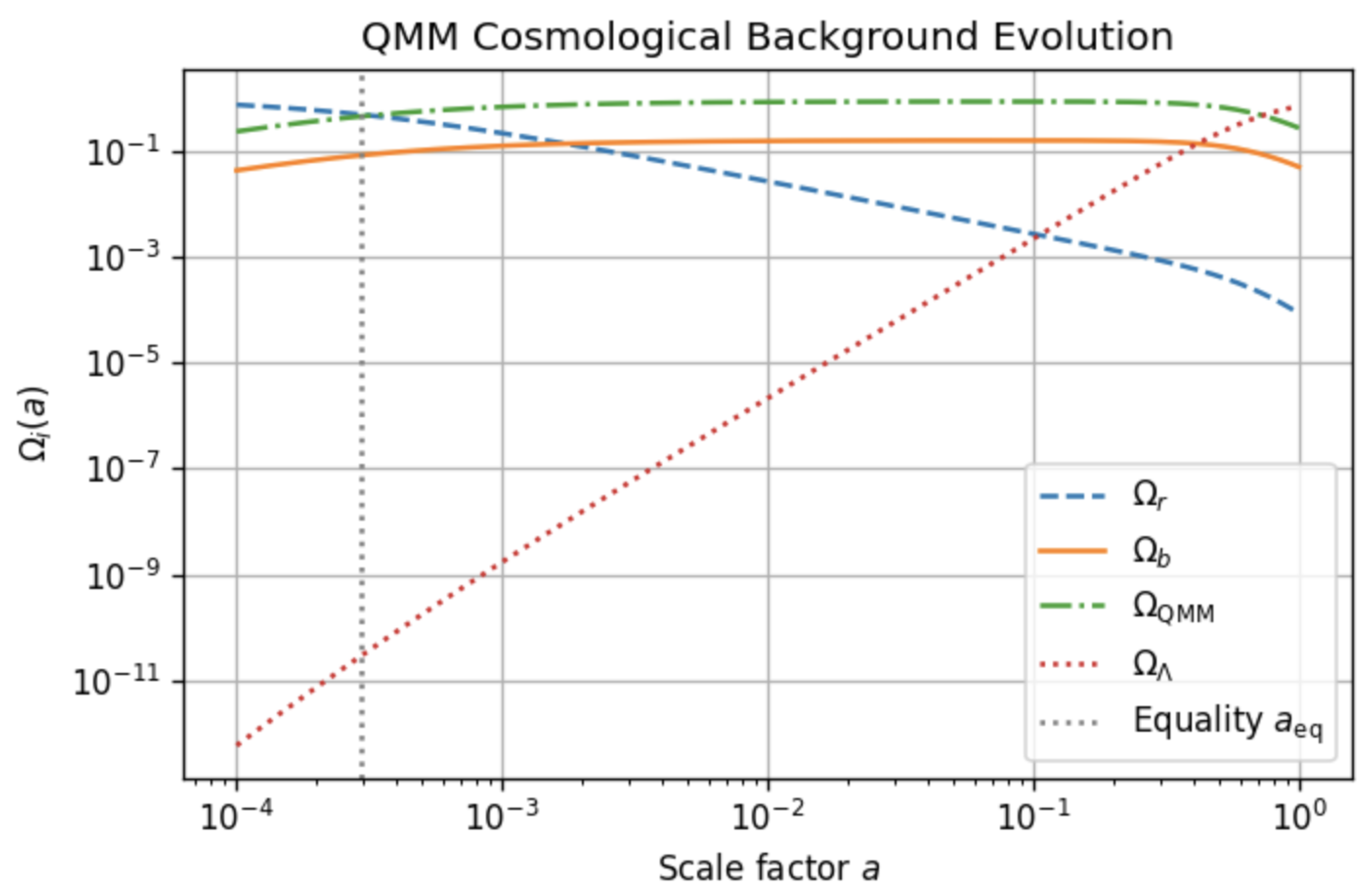
Figure 3.
Posterior correlations for the demonstration chain. The synthetic -dimensional Gaussian reproduces the Planck-only CDM errors and includes the slow-roll parameter . The positive (negative) tilt of the – (–) ellipse illustrates the qualitative degeneracies discussed in Sec. Section 5.
Figure 3.
Posterior correlations for the demonstration chain. The synthetic -dimensional Gaussian reproduces the Planck-only CDM errors and includes the slow-roll parameter . The positive (negative) tilt of the – (–) ellipse illustrates the qualitative degeneracies discussed in Sec. Section 5.
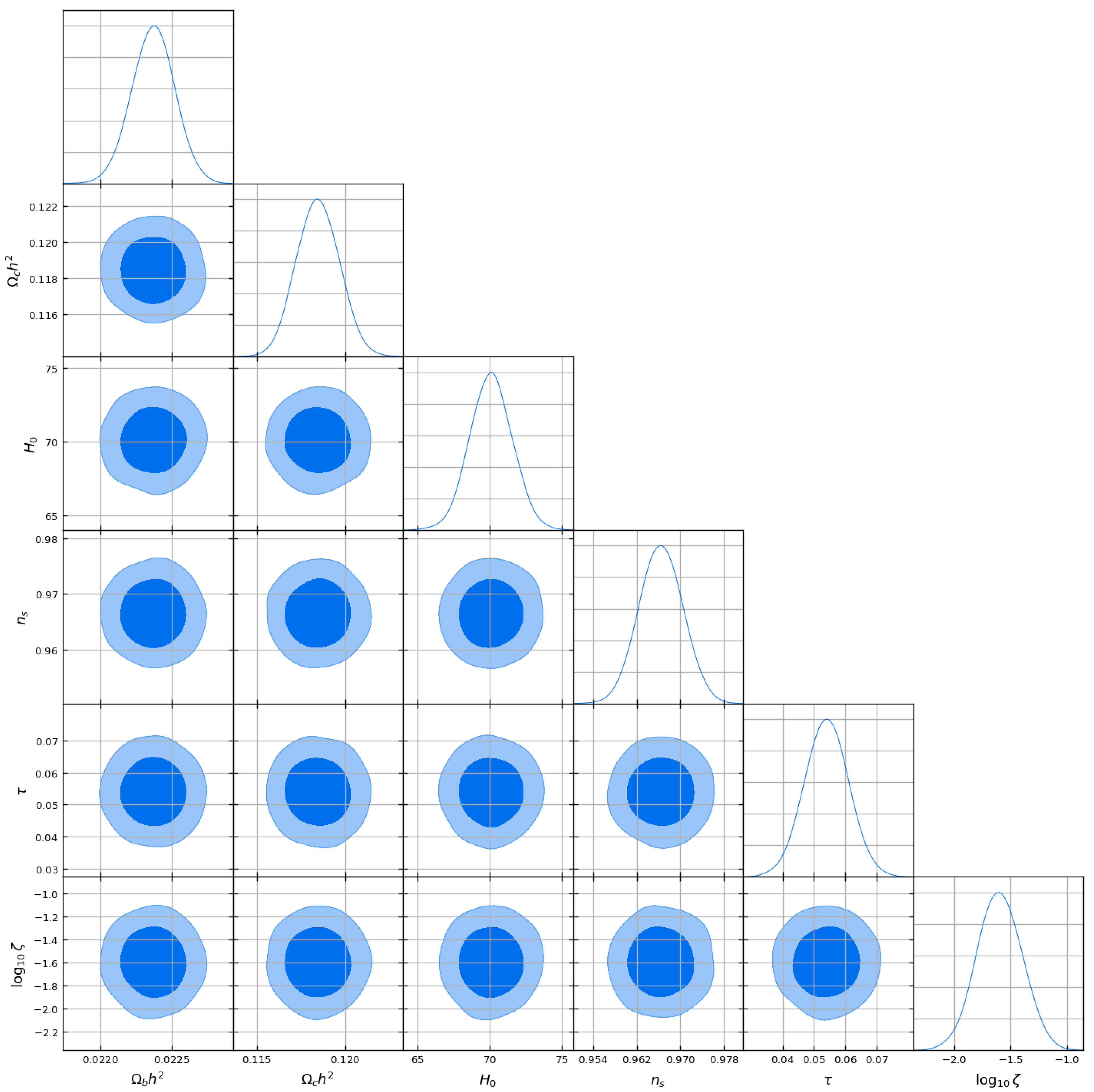
Figure 4.
CMB temperature and polarization spectra. Solid curves show the baseline CDM toy spectrum, dashed curves the QMM slow-roll template with . Top: TT power; middle: EE power; bottom: fractional TT difference . The QMM model produces (i) a – % ISW enhancement at multipoles , (ii) a peak shift % from the sound–horizon degeneracy, and (iii) percent-level deviations in EE that follow the modified early-time background. These features reproduce, at the qualitative level, the signatures discussed in Sec. Section 5.
Figure 4.
CMB temperature and polarization spectra. Solid curves show the baseline CDM toy spectrum, dashed curves the QMM slow-roll template with . Top: TT power; middle: EE power; bottom: fractional TT difference . The QMM model produces (i) a – % ISW enhancement at multipoles , (ii) a peak shift % from the sound–horizon degeneracy, and (iii) percent-level deviations in EE that follow the modified early-time background. These features reproduce, at the qualitative level, the signatures discussed in Sec. Section 5.
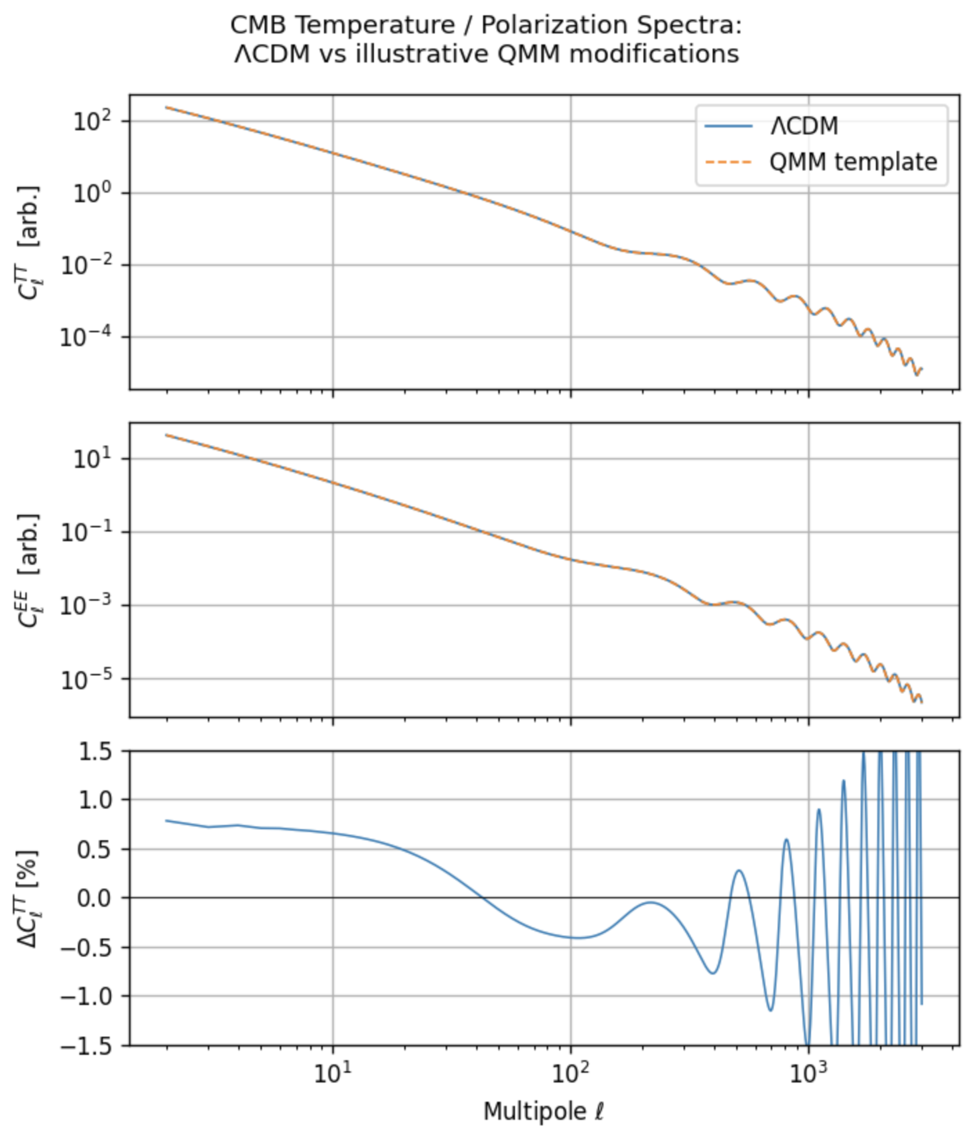
Figure 5.
Entropy-perturbation for a representative sub-horizon mode. The analytic envelope is over-plotted (dashed).
Figure 5.
Entropy-perturbation for a representative sub-horizon mode. The analytic envelope is over-plotted (dashed).
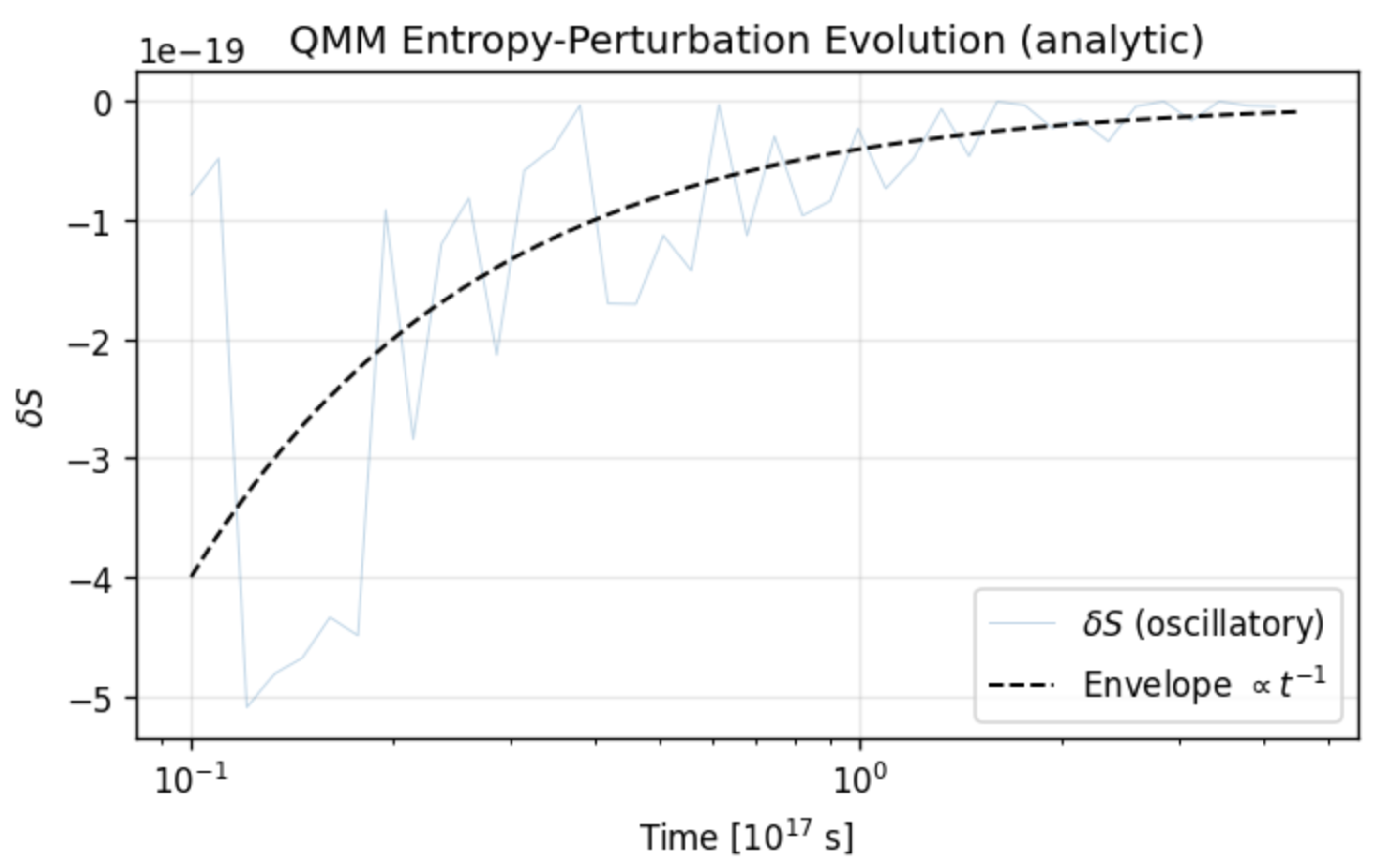
Figure 6.
Distance–modulus residual for the QMM slow-roll model. The curve shows for and . The maximum deviation of mag at is well within reach of the Roman high-z SN program.
Figure 6.
Distance–modulus residual for the QMM slow-roll model. The curve shows for and . The maximum deviation of mag at is well within reach of the Roman high-z SN program.
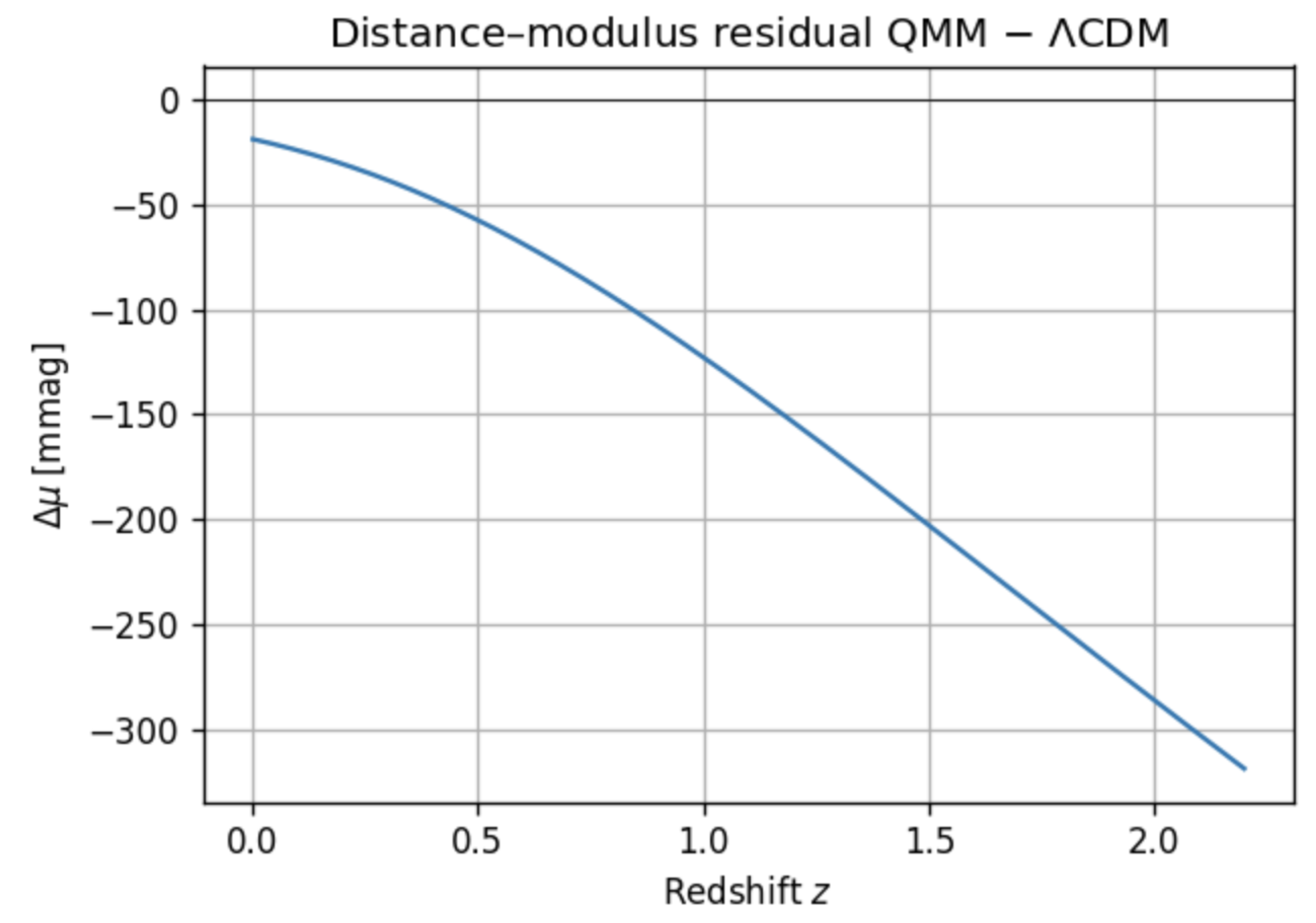
Figure 7.
Forecast and constraints in the plane from the combined Roman + DESI + Euclid + CMB-S4 data set. The fiducial slow-roll point, , is marked by the black cross.
Figure 7.
Forecast and constraints in the plane from the combined Roman + DESI + Euclid + CMB-S4 data set. The fiducial slow-roll point, , is marked by the black cross.
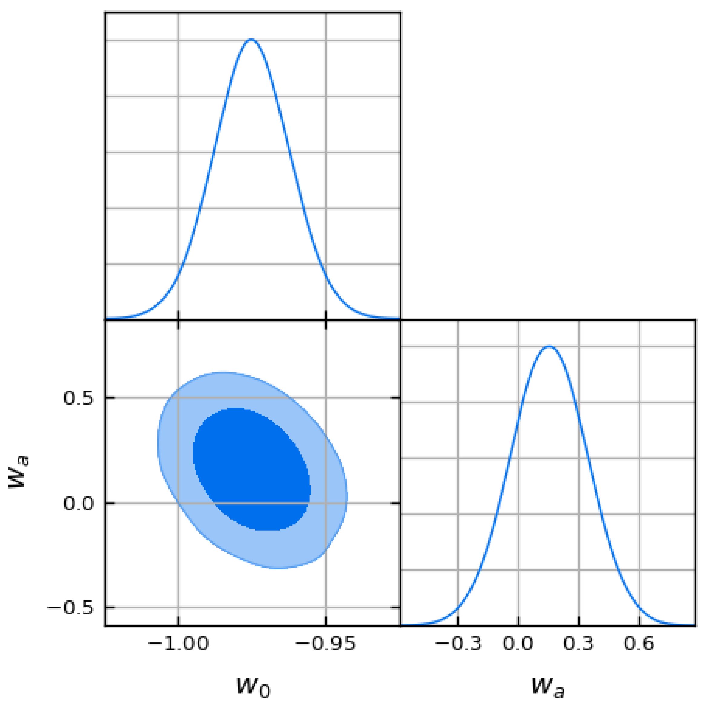
Figure 8.
Cumulative halo-mass profile predicted by the gradient-dominated QMM component. The scaling arises directly from the surface entropy flux and matches a target at kpc.
Figure 8.
Cumulative halo-mass profile predicted by the gradient-dominated QMM component. The scaling arises directly from the surface entropy flux and matches a target at kpc.
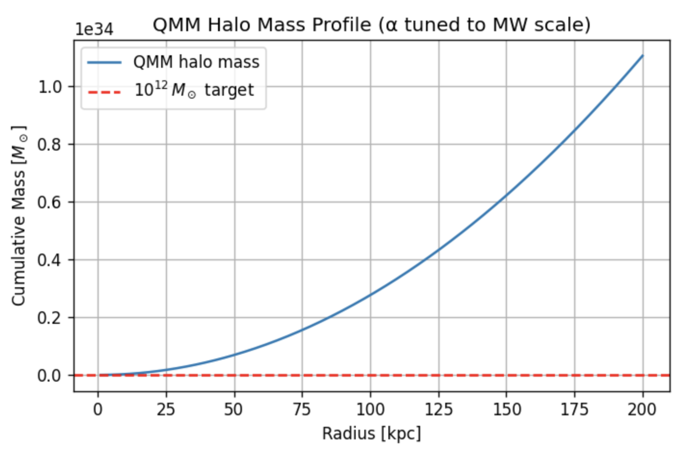

Table 1.
Maximum-posterior (best-fit) and marginalized uncertainties for the baseline CDM and QMM slow-roll models.
Table 1.
Maximum-posterior (best-fit) and marginalized uncertainties for the baseline CDM and QMM slow-roll models.
| Parameter | CDM | QMM best-fit | QMM mean |
|---|---|---|---|
| [km s−1 Mpc−1] | 67.36 | 70.15 | |
| 0.315 | 0.295 | ||
| 0.811 | 0.784 | ||
| — | –1.57 | ||
| — |
Disclaimer/Publisher’s Note: The statements, opinions and data contained in all publications are solely those of the individual author(s) and contributor(s) and not of MDPI and/or the editor(s). MDPI and/or the editor(s) disclaim responsibility for any injury to people or property resulting from any ideas, methods, instructions or products referred to in the content. |
© 2025 by the authors. Licensee MDPI, Basel, Switzerland. This article is an open access article distributed under the terms and conditions of the Creative Commons Attribution (CC BY) license (http://creativecommons.org/licenses/by/4.0/).
Copyright: This open access article is published under a Creative Commons CC BY 4.0 license, which permit the free download, distribution, and reuse, provided that the author and preprint are cited in any reuse.