
Submitted:
18 July 2025
Posted:
21 July 2025
You are already at the latest version
Abstract
State highway agencies usually measure Annual Average Daily Traffic (AADT) using traffic data from permanent detector stations that are part of their system-wide traffic monitoring programs. Agencies also estimate the AADT at many other locations using short-term counts. Traffic counters at the permanent stations frequently malfunction and result in periods of inaccurate or missing data. This study used extensive traffic data from permanent detector stations in the state of Montana to examine the effect of missing data on the accuracy of AADT estimation. On a rotational basis, one station was used for testing the accuracy of AADT estimation, while the remaining stations (training stations) were used in developing the traffic adjustment factors. Data trunca-tion at the training stations was conducted using two sampling techniques and three scenarios of data availability. The study results showed that the increase in AADT ap-proximation (inaccuracy) was not linearly proportional to the increase in the amount of missing data. Given the extreme scenarios of missing data examined in this study and the relatively lower effect on AADT approximation, it can be concluded that the current practice in treating missing data does not involve a considerable compromise in the accuracy of AADT estimation.
Keywords:
traffic monitoring program
; AADT
; missing data
; adjustment factors
; traffic data collection
; permanent stations
1. Introduction
State highway and transportation agencies implement systemwide traffic monitoring programs for collecting traffic data such as vehicle speed, weight, classification, and traffic volume. The Federal Highway Administration (FHWA) has provided guidance on the planning, development, and continued operation of traffic monitoring programs for state transportation agencies. As a result, each state records traffic data as part of the traffic monitoring program to meet the FHWA traffic data reporting requirement. This data serves as the backbone of many agency programs such as transportation planning, design, operation, and management.
Traffic volume, in the form of the annual average daily traffic (AADT), serves as the critical output of traffic monitoring programs. The AADT is calculated using the total traffic in both directions of travel over one full year divided by 365. Accurate AADT estimation is crucial for sustainable transportation planning, ensuring reliable traffic assessments and informed infrastructure management. Transportation professionals at all levels know the importance of AADT data [1]. It is a fundamental metric in many applications, such as pavement and highway design, traffic operations, transportation planning, and fuel-tax revenue projections (to name but a few). Collecting comprehensive traffic data is often impossible due to associated costs [2]. Despite the challenge, it is crucial to have a reasonably accurate estimate of the AADT, and therefore, agencies allocate substantial portions of the available resources to various data collection programs [3].
There are two primary types of traffic counts: continuous counts (often known as control counts) at a limited number of permanent counting sites, and short-term counts (often known as coverage counts) at a more significant number of temporary counting sites throughout the network. Short-term counters collect data over a period ranging from 1 to 7 days (typically 48 hours) [4]. These counters provide a sample of traffic volume over a greater extent of the highway network. Short-term counts must be seasonally adjusted to better represent traffic conditions over a typical day. However, permanent traffic counters typically collect data hourly or at 15-minute intervals, seven days a week, and for 365 days a year. These provide a measure of variation in traffic patterns accounting for daily, weekly, and monthly temporal variations.
Data collection techniques are varied from manual devices to advanced detectors, sensors, and data recorders. Two fundamental types of data collection systems have been used at permanent sites in a continuously monitored highway network: Automatic Traffic Recorder (ATR) and Weigh-in-Motion (WIM). Due to the critical environment in which these systems are operated, they are highly prone to breakdown, resulting in specific periods of inaccurate or missing data. The existence of inaccurate or missing data often affects the quality and usefulness of the collected traffic data. Therefore, missing or unusable data poses a significant challenge in accurately assessing traffic volumes and adjusting traffic counts, underscoring the importance of reliable and well-maintained data collection systems.
2. Background
Data collection and management methods have evolved significantly since the 1930s [5]. Summary statistics played a crucial role in the early stage of AADT process development. In the 1930s, AADT data collection relied mainly on manual counting, which later evolved into mechanical measurement in the 1940s. The next few years saw the establishment of theoretical frameworks for AADT summary statistics and calculations. David Albright noted certain procedural uncertainties, which remained unchallenged until the late 1980s [5]. There was a lack of universal methods for calculating adjustment factors for collected traffic data [6]. Currently, many states depend on the FHWA Traffic Monitoring Guide (TMG) to obtain corrected data. The selection of sampling and AADT estimation techniques is left to the judgment of the transportation agencies.
A factoring approach is extensively used in the United States as recommended by the AASHTO Guidelines for Traffic Data Programs [7] and the FHWA’s Traffic Monitoring Guide [8]. This approach uses permanent stations to develop group adjustment factors, which are then applied to the short-term counts to estimate AADT. Traditionally, monthly and daily adjustment factors are calculated and multiplied by short-term counts to estimate AADT.
Due to malfunctions in traffic counting devices such as Automatic Traffic Recorders (ATRs) and Weigh-in-Motion stations (WIMs), data for specific periods may be missed or may not be accurately captured. Zhong et al. (2005a) conducted an in-depth analysis of the counting efficiency of Alberta’s continuous traffic counting program. The results revealed that the data sets frequently have missing portions of data. For instance, in 1998, over 56% of Automatic Traffic Recorders (ATRs) had missing records, and nearly 35% contained less data than required by the AASHTO’s Guidelines for Traffic Data Programs for generating group expansion (adjustment) factors [10]. In most cases, deploying additional traffic counting devices to complete the data set is unrealistic, and discarding a substantial portion of successfully collected data is undesirable. Therefore, many agencies resort to estimating missing values in collected traffic counts, a technique often called data imputation. Accurate implementation of data imputation is essential for maintaining the integrity of the data and enhancing the cost-effectiveness of traffic data monitoring programs. The AASHTO’s Guidelines for Traffic Data Programs [10] identifies two essential principles. The principle of base integrity requires that the original traffic measurements remain unaltered, with missing values not imputed in the base data. The principle of truth-in-data requires that highway agencies document procedures for editing traffic data, ensuring transparency and reliability for users in decision-making.
Research conducted by the New Mexico State Highway and Transportation Department concluded that 13 states had procedures to estimate missing values and complete the dataset when portable traffic devices failed. In comparison, 23 states had similar procedures when permanent devices failed [11,12]. In Vermont, data imputation is performed based on the data from the same day and month in the previous year. The data from the previous three years serve as the basis for estimation in South Dakota. In Montana, historical data from the same site are utilized for estimation. If no significant changes in traffic patterns have occurred, the data are directly used; otherwise, an adjustment factor is applied. In Delaware, data imputation is performed based on linear interpolation from the adjacent months. In Oklahoma, missing data estimates are derived from the data collected on the corresponding day of the week in the same month for a maximum of a 9-hour gap. In Indiana, estimations are based on data from the previous year with a maximum imputation duration of 1 week. In Alberta, missing hourly volumes are not imputed, but historical data are utilized to estimate the monthly average daily traffic (MADT). In Manitoba, the estimation is for the same hour and day of the week for the previous year. In London, the estimation is based on the hourly volume of the same hours and days of the previous week [13].
A study comparing different imputation methods used by traffic agencies analyzed ATR data from Alberta and Saskatchewan [13]. The findings indicated that methods incorporating additional information and employing advanced prediction models yielded significantly better results. Another study focused on imputing traffic count data during the holiday season highlighted the superior performance of the k-nearest neighbor (KNN) method. Another research compared several imputation methods such as expectation maximization (EM), mean, k-nearest neighbor (KNN), multivariate imputation by chained equations (MICE), random forest (RF), and median [14]. The results from the previous study showed that using the median value for imputation was the most effective approach. However, the evaluation of imputation accuracy was not conducted as an independent assessment. Instead, it was intertwined with the accuracy of predicting hourly volumes for a subsequent year. As a result, the effectiveness of the different imputation techniques might be constrained by the predictive capacity of the utilized algorithms, such as artificial neural network (ANN), long short-term memory (LSTM), gated recurrent units (GRU), and recurrent neural networks (RNN). In a more recent study, researchers devised a congestion imputation model (CIM) for traffic congestion level data, utilizing joint matrix factorization [15]. The model captured data repetition and road similarities using time-based and location-based information. Subsequently, restrictions were applied to maintain consistency over time. The findings revealed that by leveraging the attributes of congestion patterns, the model could impute missing data with greater accuracy compared to several other highly used methods.
In Australia, a recent study on imputing missing data utilized ATR data from New South Wales [16]. A random selection of 25% of the reliable data was used to test three different classes of methods (multivariate imputation by chained equations (MICE), random forest (RF) and extreme gradient boosting (XGBoost), including 13 different imputing methods. The study examined two scenarios of data omission: 25% and 100%. The results showed that the missForest method outperformed the other imputation techniques. The AADT values were computed using both the original counts before imputation and the completed counts after imputation. The AADT values derived from the imputed data were marginally higher. However, when the ADT were plotted, the quality of the imputed data was validated, as the yearly trends exhibited a comparatively better fit [16]. Another study utilized non-motorized count (bicycle and pedestrian) data from various cities in Oregon and explored multiple imputation methods [17]. The findings indicated that the random forest (RF) method yielded the best results, however, in cases of minimal missing values, negative binomial regression proved to be more effective.
Most of the studies in the literature have focused on two aspects – AADT estimation and Methods of Imputation for missing data. There is a lack of literature on the effect of missing data on the accuracy of AADT estimation.
3. Study Motivation
The accuracy of AADT estimation is expected to vary based on the missing data criteria used by highway agencies. This research aims to examine the impact of tolerating different levels of missing data on the accuracy of the AADT estimation. In the current practice, many agencies adopt the following criteria in estimating the AADT [16]:
- At least one daily volume is necessary for each day of the week (DOW) within a month.
- A minimum of 19 hourly observations must be recorded for each daily volume.
- The daily traffic volume should fall within 20% of the average for that specific day of the week in the month.
Based on these criteria, only permanent stations with at least one DOW of data in any specific month are used in developing the group adjustment factors. Given the significant missing data tolerance in the above criteria, the current research aims at assessing the impact of missing data on the accuracy of AADT estimation. Specifically, the research utilizes a case study to test the hypothesis that the more the missing data in the permanent ATR/WIM stations, the lower the accuracy in the AADT estimation process.
4. Study Approach
To investigate the impact of various levels of missing data on the AADT estimation, a group of ATRs/WIMs belonging to the same highway functional classification with complete year of traffic counts (365 days) is required. Using data from the state of Montana, it was decided to use the “Rural Principal Arterials – Others” in this investigation. These involve non-interstate major rural highways including intercity routes throughout the state. The main consideration for the selection is the higher number of ATR/WIM stations with full year traffic counts (compared to other functional classifications). Out of the stations identified with full year of traffic data, one station was used for validation and testing (later called testing station) while the rest of the stations were used in developing the traffic (or the group) adjustment factors (later called training stations). The process was repeated multiple times, ensuring that each station was used as a testing station once while included in the training stations for all other iterations. The data at the training stations is then truncated to reflect the different levels of missing data and the AADT for the testing station is estimated and compared with the actual value. Three levels of available (or missing) data were used: one week, two weeks, and three weeks of available data in any given month. To remove any potential bias in truncating the data, two random sampling techniques were used consistently with each level of missing data:
- i.
- Sampling technique I: In this technique, random days within a specific month are selected to represent the level of available (or missing) data. For instance, one week of available data would include one Monday, one Tuesday, one Wednesday, etc., all selected randomly within the month.
- ii.
- Sampling technique II: In this technique, the duration of the available data (one, two, or three weeks) is selected randomly within the month as a continuous period of time. This sampling approach seems more realistic as the periods when ATRs or WIMs are down, or malfunction tend to be continuous within any given month.
For each sampling technique, a large number of scenarios/simulations was considered following the law of larger numbers in statistics, which states that as the number of trials increases, the mean of results becomes more accurate and converges to the expected value [18]. In this research, one hundred simulations were used in generating the Monthly Day of the Week (MDOW) adjustment factors. Therefore, this process yielded a hundred sets of MDOW adjustment factors for each iteration.
The next step is the testing/validation of the AADT approximation using actual traffic counts at the testing station for each iteration. Using the 100 sets of MDOW adjustment factors, the percent approximation (% discrepancy) was calculated 100 times for each day of the year (daily volume treated as a short-term count) and absolute values were averaged to represent the % discrepancy for that particular day. The final step was to find the average discrepancy in AADT estimation for each level of missing data over one full year using the mean absolute value of daily discrepancies found in the previous step.
4. Data Collection
Data was acquired using the data collection program of the Montana Department of Transportation (MDT). Upon examining available ATR and WIM data from 2019 to 2023, the functional class of “rural principal arterial-Other” for the year 2022 was selected for use in this research. This functional class involves all non-interstate rural principal arterials including major intercity routes. The year 2022 was considered for the higher number of ATR/WIM stations with full year of continuous traffic data. Specifically, for the year 2022, there were 65 active permanent stations: 25 ATRs and 40 WIMs, but only 17 stations had a full year of data. Among those 17 stations, 10 of them belonged to the “Rural Principal Arterials – Other” classification. As stated earlier, out of these 10 stations, 9 were considered for training and 1 for testing purposes. Figure 1 shows the location of the 10 ATR and WIM stations used in this research (4 ATR sites labeled as “C” and 6 WIM sites labeled as “W”). The data collected was 365 days of traffic volume for each vehicle class (classes 1 to 13) at the ten permanent stations.
5. Analysis And Results
This section summarizes the results of the study that are presented in separate subsections. Specifically, a base scenario is presented where no missing data is considered and used as a benchmark for AADT approximation evaluation. Afterwards, results from the scenarios with different levels of missing data are presented.
5.1. Base Condition (No missing Data)
The base condition assumes that the MDOW adjustment factors are developed from permanent stations with a full year of traffic data. This scenario is important as it serves as a reference in assessing the discrepancy in AADT estimation using different levels of missing data. Adjustment factors for each of the nine training stations were calculated through a factoring approach (outlined in the FHWA Traffic Monitoring Guide) and then averaged into one set of 84 MDOW adjustment factors. For the testing station, the daily total vehicle count was considered a short-term count for the day, and using adjustment factors from the training stations, AADT was calculated by multiplying the short-term count for each day with the respective adjustment factor. The AADT was estimated for each of the 365 days in the testing dataset. As the actual AADT was already known, the percentage discrepancy was calculated between the actual AADT and the estimated AADT for each day and then averaged over the entire year. For the base condition, the mean absolute percent discrepancy between the actual AADT and the estimated AADT at the testing stations are shown in Table 1.
5.2. Scenario 1 (Permanent stations with one week of data per month)
This scenario considered a total of one week of available traffic data per month, totaling 84 days of traffic data annually - an extreme case showing minimum data availability. As stated earlier, two random sampling techniques were applied in running the analysis, and 100 simulations of random selections were used in the analysis. Figure 2 shows the mean absolute percent discrepancy (for each iteration) using the two sampling techniques along with the result for base condition. This scenario of missing data (scenario 1) shows a notable increase in AADT approximation (% discrepancy) in comparison to the base condition. The sampling technique I was found to have slightly lower % discrepancy compared with the sampling technique II in eight of the ten testing stations and almost identical (no difference) in the remaining two stations.
To test whether the difference in means of both sampling techniques was statistically significant, a two-tailed t-test was performed, and results are shown in Table 2. The t-test revealed no statistically significant difference between the mean of sampling technique I, and the mean of sampling technique II for any testing station at the 95% confidence level. Therefore, it can be concluded that there is no evidence of a statistical difference between the mean percent discrepancy of the two sampling techniques. A one-tailed t-test was also conducted to compare the mean discrepancy of the base condition with the mean of scenario I using sampling techniques I and II as shown in Table 2. The tests revealed no statistically significant increase in the mean discrepancy for scenario I at the 95% confidence level using sampling techniques I or II at all testing stations except stations A-008 and W-101.
Figure 3 shows the daily discrepancies for station A-046 between the actual and estimated AADT for sampling technique II (scenario 1). Sampling technique II was selected as it is more realistic and more likely to occur compared to scenario I. A positive percent discrepancy denotes the occurrence where the estimation method underestimates the AADT while a negative percent discrepancy indicates an AADT overestimation. The figures show a large fluctuation in percent discrepancy when applying adjustment factors on different days throughout the year. A careful examination of Figure 3 shows that the months of July and August, the peak travel season, were largely associated with positive discrepancies, along with the months of January and December. On the other hand, negative percent discrepancies were overrepresented during the off-peak fall season from late September to late November, as well as during the month of March.
5.3. Scenario 2 (Permanent Stations with Two Weeks of Data Per Month)
Using two weeks of available data in every month of the year, the AADT approximation was analyzed, and results are presented in this section. Figure 4 shows the mean absolute percent discrepancy in AADT estimation for the base condition and the two weeks data availability using the two sampling techniques.
At a glance, it is clear that the missing data had a negative impact on the AADT estimation as exhibited by the higher percent discrepancy. Further, similar to scenario 1 analysis, the sampling technique I (random days of week) yielded lower AADT approximation than sampling technique II (random period within the month) in eight of the ten testing stations.
T-tests were conducted to examine whether missing data and sampling techniques used have significant effect on mean discrepancy in AADT estimation. Consistent with the t-test results of Scenario I, the two-tailed t-test revealed no statistically significant difference between the mean discrepancy using sampling techniques I and II at the 95% confidence level. Further, a one-tailed t-test was also conducted to compare the mean discrepancy of the base condition with the means of sampling technique I and sampling technique II as shown in Table 3. The tests revealed no statistically significant increase in the mean discrepancy for sampling technique I or for sampling technique II at the 95% confidence level for any of the ten testing stations.
Figure 5 shows the daily percent discrepancies for station A-046 between the actual and estimated AADT for scenario 2 using the sampling technique II. The patterns exhibited in Figure 3 are largely similar to those shown in Figure 5. Specifically, the AADT is often underestimated during the peak summer season in July and August as well as towards the start and end of the year, while AADT overestimation is evident in the fall months of October and November as well as in March.
5.4. Scenario 3 (Permanent Stations with Three Weeks of Data Per Month)
This scenario involved the least amount of missing data among those considered in this study. Figure 6 shows the mean absolute percent discrepancy in AADT estimation for the base condition and three weeks of data availability using the two sampling techniques.
The patterns exhibited in Figure 6 are very similar to those exhibited in Figure 2 and Figure 4. Specifically, the base condition is associated with the least discrepancy in AADT estimation and the sampling technique I showed lower discrepancy in AADT estimation compared to sampling technique II in eight of the ten testing stations.
Similar to the previous scenarios, the two-tailed t-test revealed no statistically significant difference between the mean discrepancy of sampling technique I and that of sampling technique II at the 95% confidence level, as shown in Table 4. Therefore, it can be concluded that there is no evidence of a statistical difference between the mean percent discrepancy of the two sampling techniques at the 95% confidence level at all testing stations. A one-tailed t-test was also conducted to compare the mean of the base condition with that of scenario 3 using sampling techniques I and sampling technique II. The tests revealed no statistically significant increase in mean discrepancy for scenario 3 using sampling techniques I or II at the 95% confidence level.
Figure 7 shows the daily percent discrepancies for station A-046 between the actual and estimated AADT for scenario 3 using sampling technique II. Similar to the previous scenarios, AADT underestimation occurred more often during July and August as well as during January and December, while AADT overestimation was more notable during the fall (October and November) as well as during March.
The analysis of the three scenarios consistently showed an impact of missing data on the accuracy of AADT estimation. In order to examine the impact of the level of missing data on AADT estimation, the mean absolute percent discrepancy between the actual and estimated AADT at all testing stations were averaged for each scenario and the results are shown in Figure 8 with the exact values provided in Table 5. Figure 8 clearly displays a pattern of decreasing mean percent discrepancy with the increase in scenario number, as we move from scenario 1 to scenario 3. This pattern is consistent with the expectation that the greater the amount of missing data, the lower the accuracy in AADT estimation and the greater the mean absolute percentage discrepancy between the actual and estimated AADT. This observation is applicable to the results of the two sampling techniques used in this study.
A careful examination of Table 5 reveals another important observation that has implication on the AADT estimation in practice. Specifically, despite the dramatic scenarios of missing data used in the study, the increase in the mean discrepancy of AADT estimation compared to the base condition (values shown in brackets) are modest in general, as it varied in the range of 0.68% (around 31% missing data) to 6.67% (around 77% missing data). This shows that the current practice of using a minimum of one weekday in a month adopted by some state agencies is unlikely to result in any important compromise in AADT estimation. This is particularly true given the extreme scenarios tested in this study, i.e., the data are missing at all training stations simultaneously throughout the whole year, which is unlikely to occur in real life. The percent increase in AADT approximation for the different levels of missing data and the two sampling techniques is shown in Figure 9.
A two-way ANOVA was conducted to examine the effects of missing data and sampling technique on the mean absolute percent discrepancy for each testing station. The results of the ANOVA for station A-046 are summarized in Table 6. The effects of missing data and sampling technique on the mean absolute percent discrepancy were not found statistically significant, with p-values of 0.272 and 0.586, respectively. Moreover, the interaction between missing data scenarios and sampling techniques was not found statistically significant with a p-value of 1. This indicates that the effect of sampling techniques on the mean absolute percent discrepancy did not depend on scenarios, and vice versa. Similar results were found for other testing stations.
It is also of interest to examine whether the level of missing data has any influence on the variability of AADT approximation. Figure 10 shows the standard deviation of the mean absolute percent discrepancy for the various scenarios of missing data for station A-046 using the two sampling techniques. Results show that the highest level of missing data (scenario 1) is associated with higher standard deviation and variability in AADT approximation. The other two levels of missing data (scenarios 2 and 3) are associated with lower variability in AADT approximation with the standard deviation of mean absolute discrepancy being almost equal. Regarding the effect of sampling technique on variability in discrepancy of AADT estimation, Figure 10 shows higher variability for sampling technique II with higher standard deviations for the various levels of missing data. Both sampling techniques exhibit a very similar pattern in the variability of AADT approximation.
Figure 11 shows the mean absolute percent discrepancy for station A-046 and the coefficient of variation by month of the year along with the ratio of the monthly average daily traffic (ADT) to the AADT. The figure clearly shows that the mean absolute percent discrepancy is higher during seasons of peak travel (June - July) as well as during winter months with lower traffic volumes. The coefficient of variation in monthly mean percent discrepancy varies in the range 0.6 to 0.9 throughout the year with the exception of September (highest value 1.18) and March (lowest value 0.14). The relationships shown in Figure 11 are almost identical for the three scenarios of missing data.
6. Summary And Conclusions
The annual average daily traffic (AADT) is a critical input to most transportation applications in the planning, design, and operations of highway facilities. State Departments of Transportation (DOTs) usually measure the AADT at locations of permanent ATR and WIM stations and estimate the parameter at all other locations using short-term counts (1 to 2 days in duration). To estimate AADT at short-term count locations, daily and seasonal variations in traffic at permanent stations are used in the form of adjustment factors. Traffic counters at the permanent ATR and WIM stations frequently malfunction due to wear and tear, physical damage, and/or harsh environmental conditions. This malfunction results in specific periods of inaccurate or missing data. Addressing missing data ensures AADT estimates are reasonably accurate for sustainable infrastructure management. In practice, the missing data at permanent stations is tolerated for the purpose of deriving the daily and seasonal adjustment factors as long as each month of the year has a minimum of one day of the week, i.e., one Monday, one Tuesday, etc. This practice raises questions about the impact of this rule on the accuracy of AADT estimation and whether AADT estimates are still accurate enough for the intended applications. The current study aims to answer these questions. The study used ATR and WIM data from the state of Montana to examine the effect of missing data on the accuracy of AADT estimation. Two random sampling techniques were used, and three scenarios of data availability were considered in the investigation: one, two and three weeks of available data within each month. The major findings of the study are summarized below.
- i.
- Study results clearly show that the missing data has a consistent effect on the accuracy of AADT estimation, measured using the absolute percent discrepancy between the actual and estimated AADT. This finding supports the research hypothesis that the greater the amount of missing data, the less accurate the AADT estimation. However, this effect was not found statistically significant using the two-way ANOVA analysis at the 95% confidence level.
- ii.
- The increase in % discrepancy for AADT estimation was not linearly proportional to the increase in the amount of missing data. Despite the dramatic scenarios of missing data used in the analysis (31% to 77%), the change in the AADT approximation between the highest and lowest levels of missing data was in the order of 6%.
- iii.
- Given the extreme scenarios of missing data used in the study (all permanent stations missing significant amounts of data simultaneously) and the relatively low effect on % discrepancy in AADT estimation (less than 7% discrepancy for the most extreme scenario), it is reasonable to conclude that the current practice in treating missing data does not involve an important compromise in the accuracy of AADT estimation. The finding also suggests that the data containing at least one day of the week for each month can be utilized for developing daily and seasonal adjustment factors (i.e., MDOW factors) without the need for imputing missing data.
- iv.
- Sampling technique I of selecting random days within the month was associated with lower % discrepancy in AADT estimation compared with sampling technique II of selecting a random period within the month (one, two, or three weeks).
The evaluation in this study was conducted using data exclusively from the state of Montana. The authors recommend using data from other states for a comprehensive assessment, as traffic patterns may vary in different states and regions.
Author Contributions
The authors confirm contribution to the paper as follows: study conception and design: A.A.-K.; data collection: M.F.R.Q.; analysis and interpretation of results: M.F.R.Q. and A.A.-K.; draft manuscript preparation: M.F.R.Q. and A.A.-K. All authors reviewed the results and approved the final version of the manuscript.
Funding
This research received no external funding.
Data Availability Statement
The raw data supporting the conclusions of this article will be made available by the authors on request.
Acknowledgments
The authors would like to thank Peder Jerstad of the Montana Department of Transportation (MDT) for his help in traffic data collection for this research.
Conflicts of Interest
The authors declare no conflicts of interest.
Abbreviations
The following abbreviations are used in this manuscript:
| AADT | Annual Average Daily Traffic |
| MDOW | Monthly Day of the Week |
| MDT | Montana Department of Transportation |
| FHWA | Federal Highway Administration |
| ATR | Automatic Traffic Recorder |
| WIM | Weigh-in-Motion |
References
- Sharma SC, Lingras P, Liu GX, Xu F. Estimation of Annual Average Daily Traffic on Low-Volume Roads: Factor Approach Versus Neural Networks. Transportation Research Record: Journal of the Transportation Research Board. 2000 Jan 1;1719(1):103–11. [CrossRef]
- Zhao F, Chung S. Contributing Factors of Annual Average Daily Traffic in a Florida County: Exploration with Geographic Information System and Regression Models. Transportation Research Record: Journal of the Transportation Research Board. 2001 Jan 1;1769(1):113–22. [CrossRef]
- Sun X, Das S. Estimating Annual Average Daily Traffic for Low-Volume Roadways: A Case Study in Louisiana. In: 12th International Conference on Low-Volume Roads. 2019. Available from: https://trid.trb.org/View/1689977.
- Robichaud K, Gordon M. Assessment of Data-Collection Techniques for Highway Agencies. Transportation Research Record: Journal of the Transportation Research Board. 2003 Jan 1;1855(1):129–35. [CrossRef]
- Albright, D. History of estimating and evaluating annual traffic volume statistics. Transportation Research Record: Journal of the Transportation Research Board 1991; 1305:103–7. Available from: https://onlinepubs.trb.org/Onlinepubs/trr/1991/1305/1305-013.pdf.
- Fekpe E, Gopalakrishna D, Middleton D. Final Report Prepared for Office of Highway Policy Information Federal Highway Administration U.S. Department of Transportation Washington, D.C. 2004. Highway Performance Monitoring System Traffic Data for High-Volume Routes: Best Practices and Guidelines.
- Vandervalk-Ostrander A, American Association of State Highway and Transportation Officials, United States Federal Highway Administration, National Cooperative Highway Research Program. AASHTO Guidelines for Traffic Data Programs. Vol. 1. Washington, D.C.: PB - American Association of State Highway and Transportation Officials; 2009. Available from: http://dl1.wikitransport.ir/book/AASHTO_Guidelines_for_Traffic_Data_Programs_2009.pdf.
- Federal Highway Administration (FHWA). Traffic Monitoring Guide. 2022. Available from: https://rosap.ntl.bts.gov/view/dot/74643.
- Zhong M, Sharma S, Liu Z. Assessing Robustness of Imputation Models Based on Data from Different Jurisdictions: Examples of Alberta and Saskatchewan, Canada. Transportation Research Record: Journal of the Transportation Research Board 2005 Jan 1;1917(1):116–26. [CrossRef]
- AASHTO. AASHTO Guidelines for Traffic Data Programs - Table of Contents. 2009. Available from: http://dl1.wikitransport.ir/book/AASHTO_Guidelines_for_Traffic_Data_Programs_2009.pdf.
- Albright D. 1990 survey of traffic monitoring practices among state transportation agencies of the United States. In 1990. Available from: https://api.semanticscholar.org/CorpusID:168276711.
- Albright D. AN IMPERATIVE FOR, AND CURRENT PROGRESS TOWARD, NATIONAL TRAFFIC MONITORING STANDARDS. Ite Journal-institute of Transportation Engineers. 1991;61. Available from: https://api.semanticscholar.org/CorpusID:107206642.
- Zhong M, Sharma S, Liu Z. Assessing Robustness of Imputation Models Based on Data from Different Jurisdictions: Examples of Alberta and Saskatchewan, Canada. Transportation Research Record: Journal of the Transportation Research Board. 2005 Jan 1;1917(1):116–26. [CrossRef]
- Khan Z, Khan SM, Dey K, Chowdhury M. Development and Evaluation of Recurrent Neural Network-Based Models for Hourly Traffic Volume and Annual Average Daily Traffic Prediction. Transportation Research Record: Journal of the Transportation Research Board. 2019 Jun 2;2673(7):489–503. [CrossRef]
- Jia X, Dong X, Chen M, Yu X. Missing data imputation for traffic congestion data based on joint matrix factorization. Knowledge-based Systems. 2021; 225:107114. Available from: https://www.sciencedirect.com/science/article/pii/S0950705121003774.
- Shafique MA. Imputing Missing Data in Hourly Traffic Counts. Sensors. 2022 Dec 15;22(24):9876. Available from: https://www.mdpi.com/1424-8220/22/24/9876.
- Roll, J. Daily Traffic Count Imputation for Bicycle and Pedestrian Traffic: Comparing Existing Methods with Machine Learning Approaches. Transportation Research Record: Journal of the Transportation Research Board. 2021 Jul 27;2675(11):1428–40. [CrossRef]
- William Mendenhall RJBBMB. Introduction to Probability and Statistics. 14th ed. 2012. Available from: https://books.google.com/books/about/Introduction_to_Probability_and_Statisti.html?id=fQsKAAAAQBAJ.
Figure 1.
Study area showing selected ATR and WIM stations.

Figure 2.
Average absolute percent discrepancy for AADT estimation using base condition and scenario 1.
Figure 2.
Average absolute percent discrepancy for AADT estimation using base condition and scenario 1.
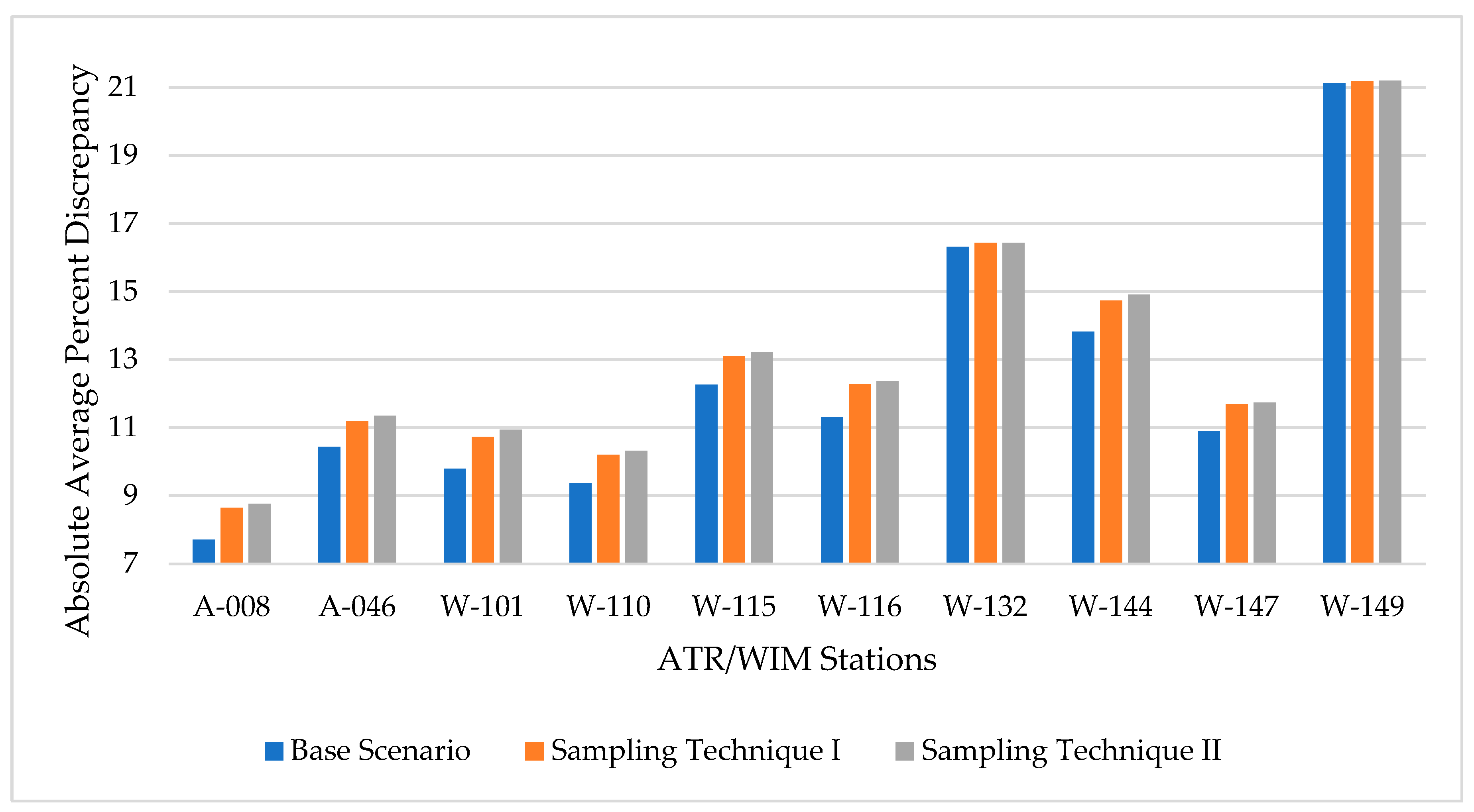
Figure 3.
Daily variation in percent discrepancies (for station A-046) using sampling technique II – Scenario 1.
Figure 3.
Daily variation in percent discrepancies (for station A-046) using sampling technique II – Scenario 1.
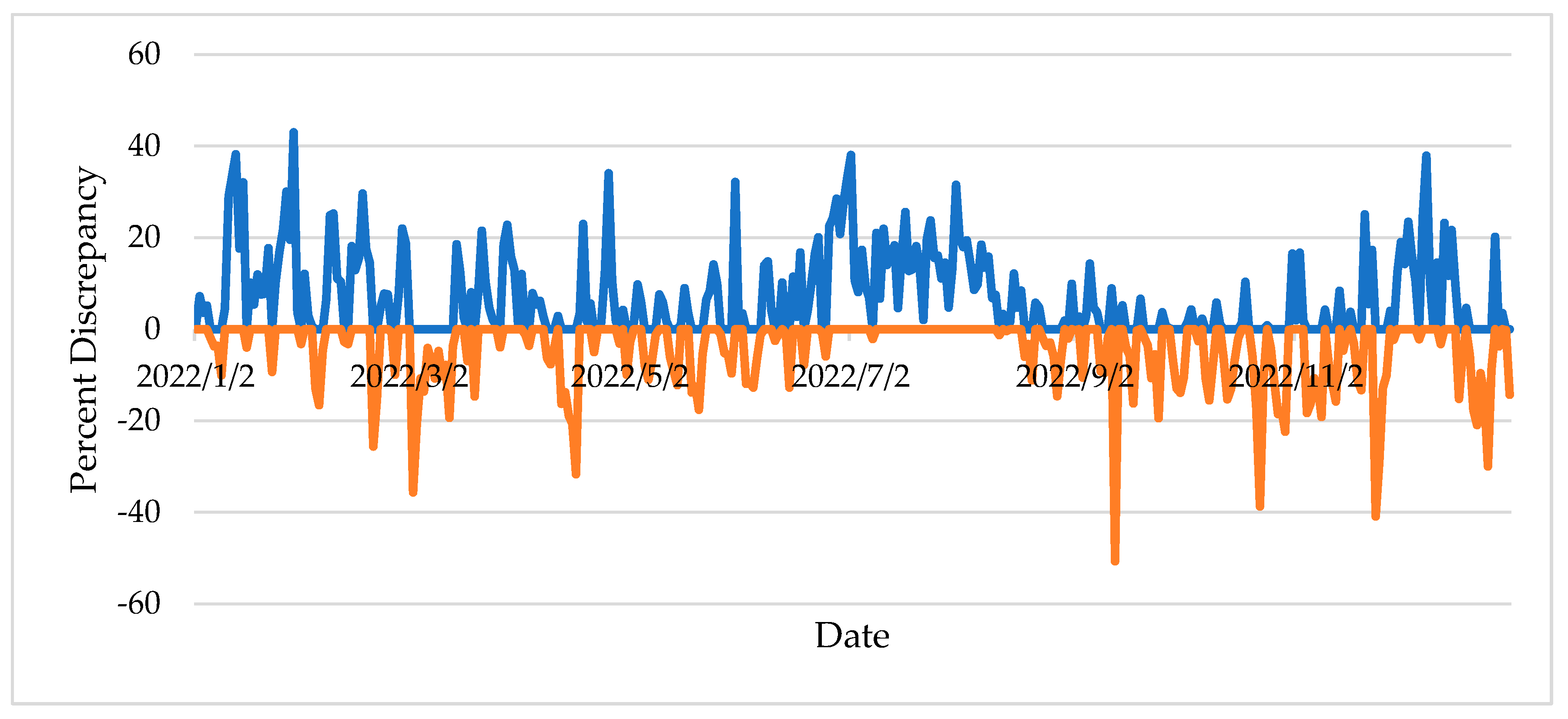
Figure 4.
Average absolute percent discrepancies for AADT estimation using base condition and scenario 2.
Figure 4.
Average absolute percent discrepancies for AADT estimation using base condition and scenario 2.
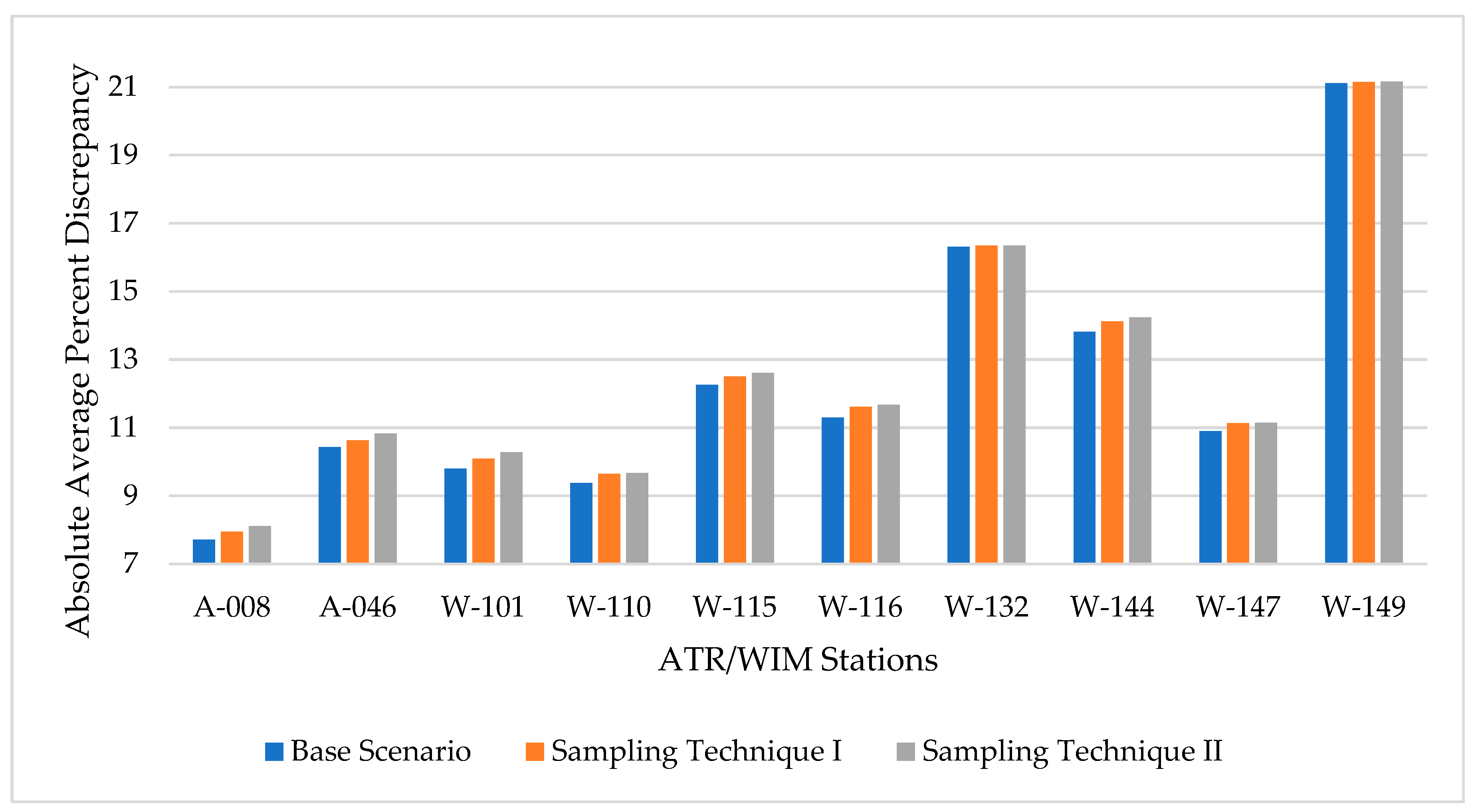
Figure 5.
Daily variation in percent discrepancies (for station A-046) using sampling technique II - scenario 2.
Figure 5.
Daily variation in percent discrepancies (for station A-046) using sampling technique II - scenario 2.

Figure 6.
Average absolute percent discrepancies for AADT estimation using base condition and scenario 3.
Figure 6.
Average absolute percent discrepancies for AADT estimation using base condition and scenario 3.
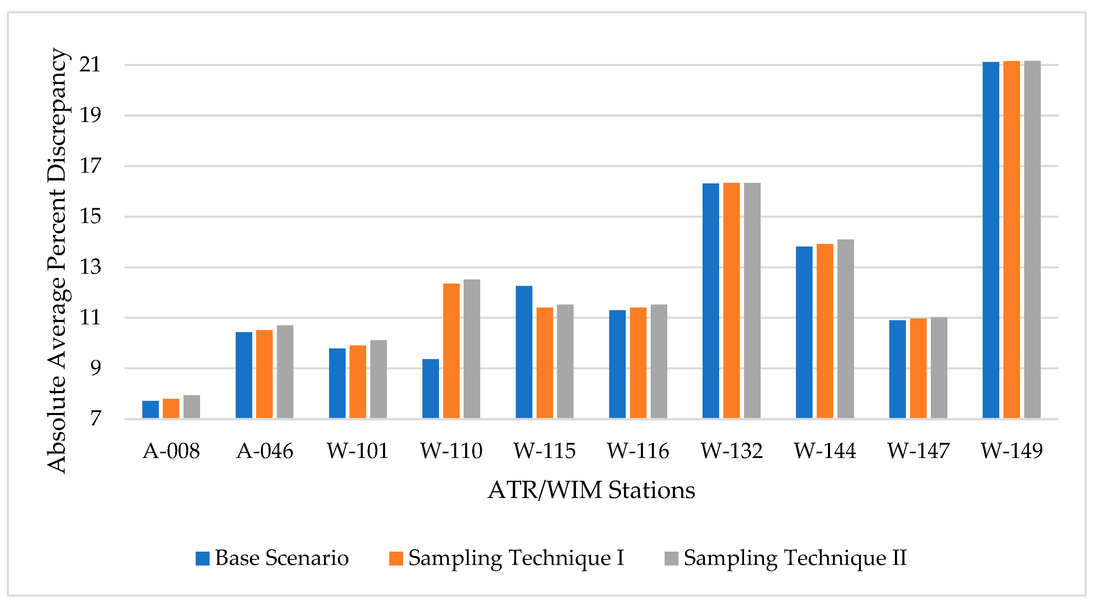
Figure 7.
Daily variation in percent discrepancies (for station A-046) using sampling technique II - scenario 3.
Figure 7.
Daily variation in percent discrepancies (for station A-046) using sampling technique II - scenario 3.
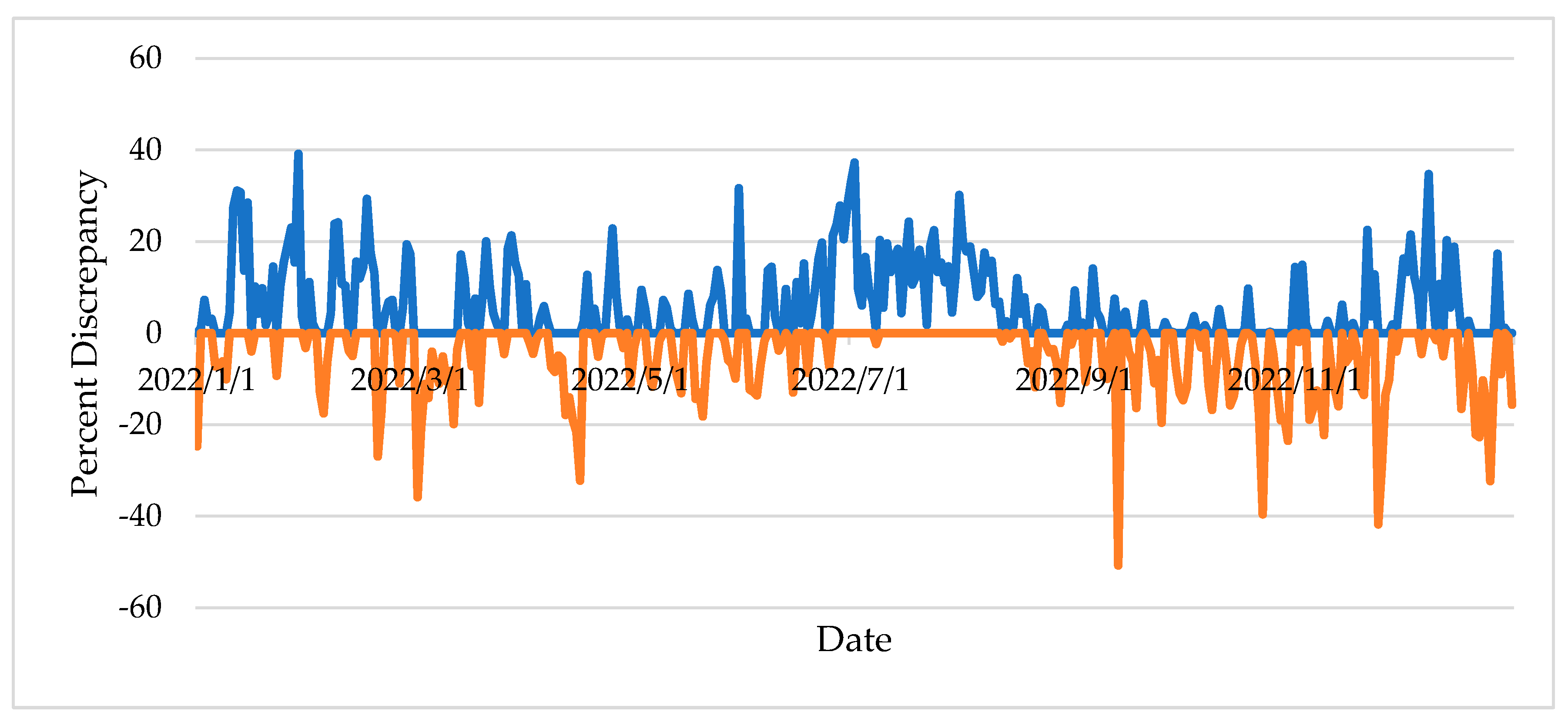
Figure 8.
Mean absolute percent discrepancy (for ten testing stations) by missing data scenario and sampling technique.
Figure 8.
Mean absolute percent discrepancy (for ten testing stations) by missing data scenario and sampling technique.
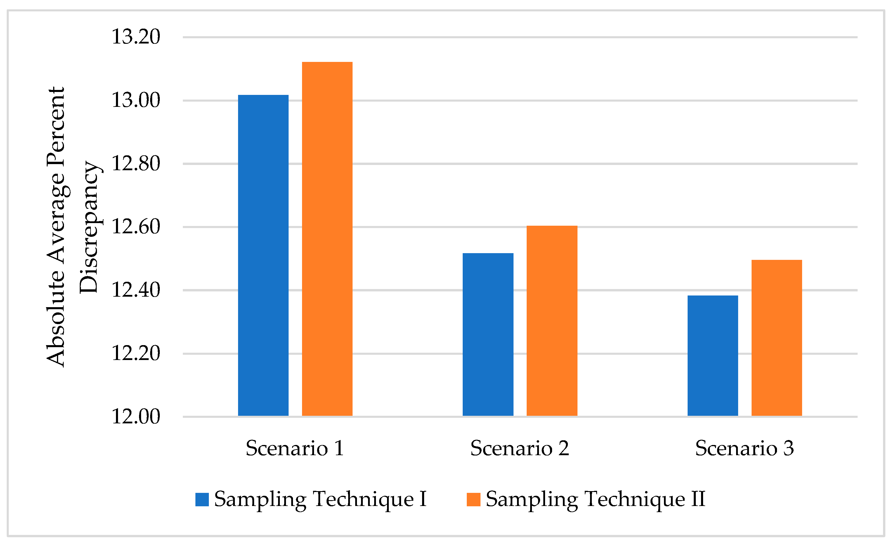
Figure 9.
Percent increase in AADT approximation compared to base condition.
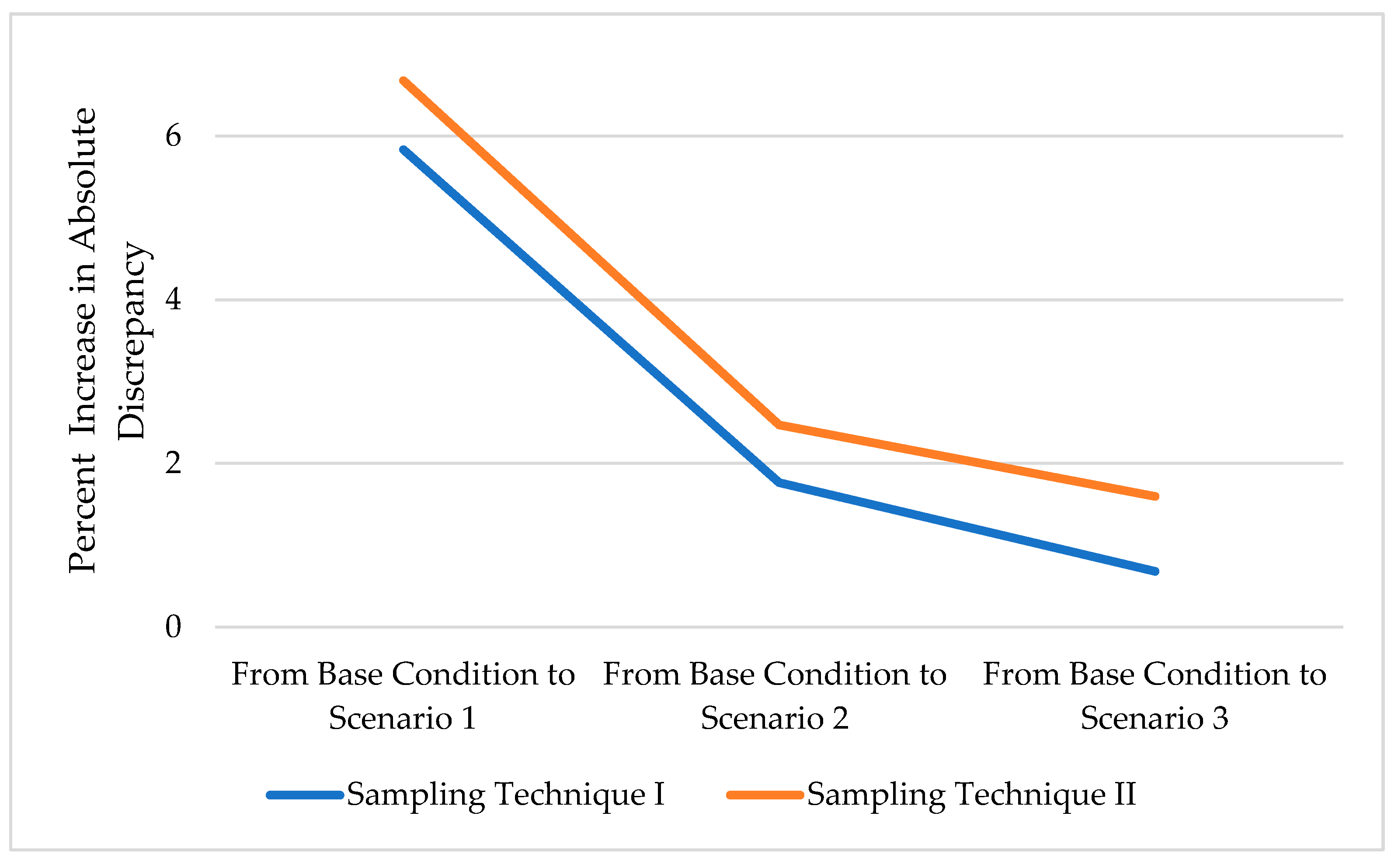
Figure 10.
Standard deviation of absolute percent discrepancy by level of missing data and sampling technique.
Figure 10.
Standard deviation of absolute percent discrepancy by level of missing data and sampling technique.
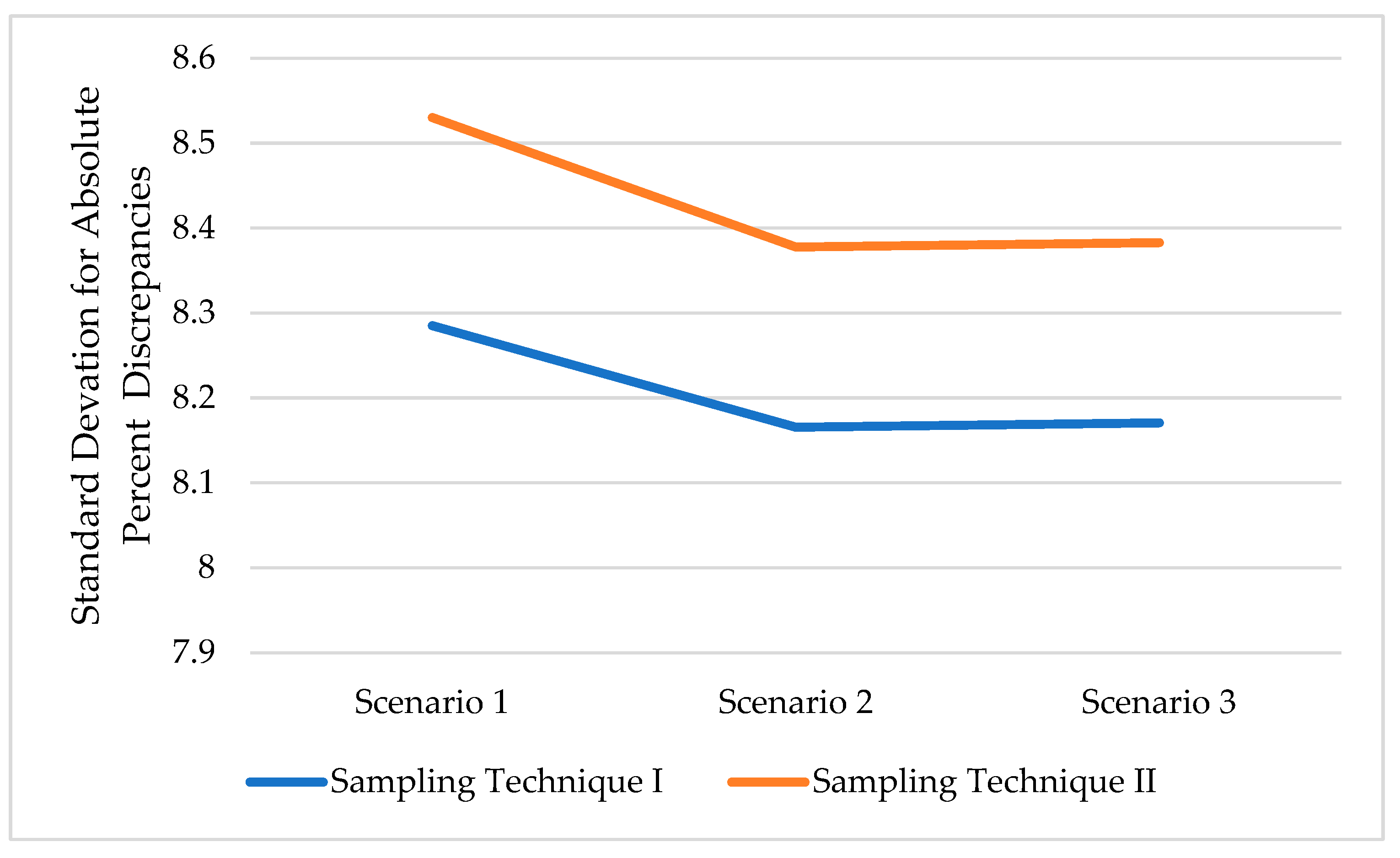
Figure 11.
Relationship between mean and CV of monthly absolute percent discrepancies (for station A-046) for sampling technique II with monthly ADT/AADT for testing station.
Figure 11.
Relationship between mean and CV of monthly absolute percent discrepancies (for station A-046) for sampling technique II with monthly ADT/AADT for testing station.
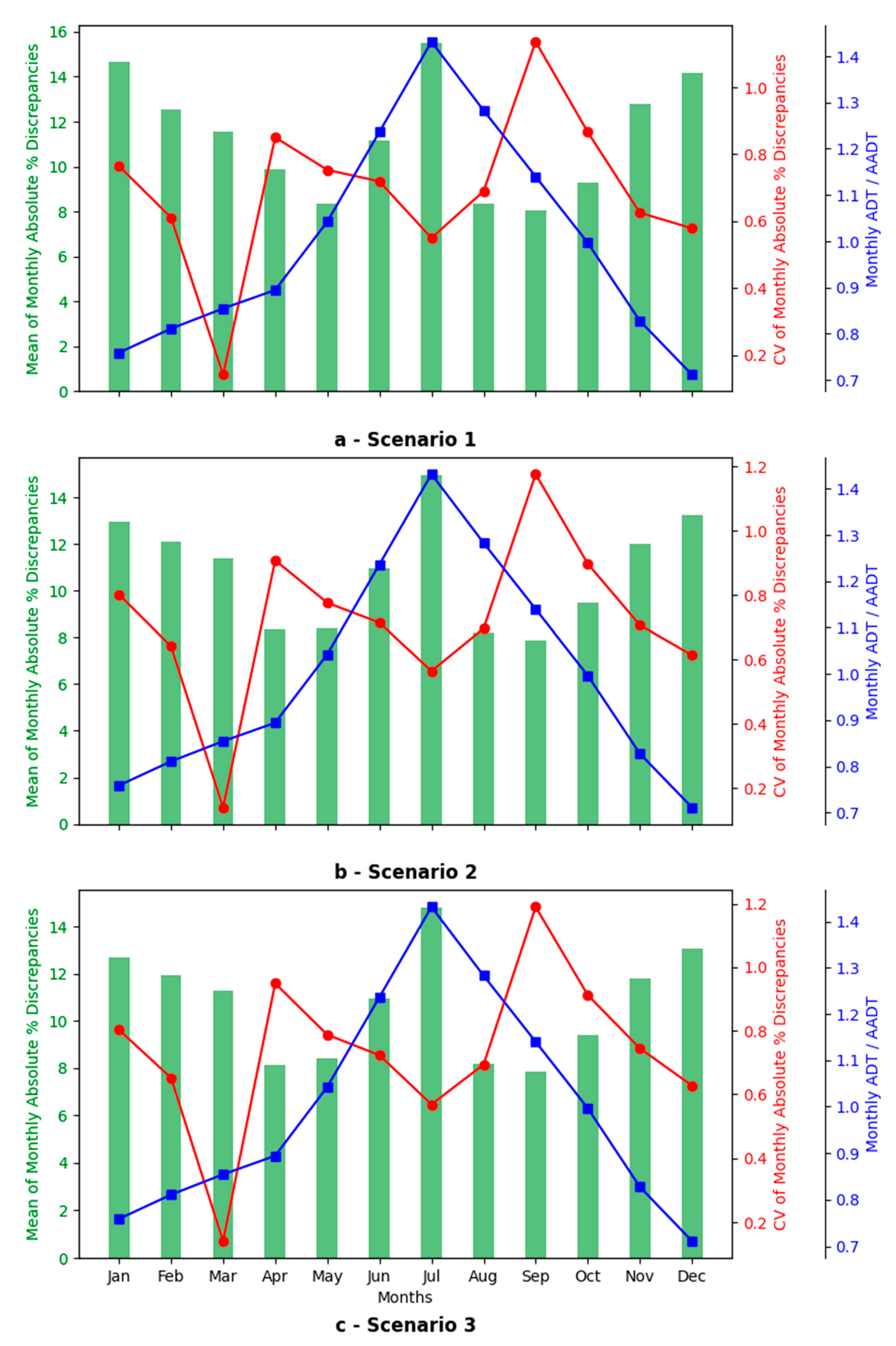

Table 1.
Average absolute percent discrepancy for AADT estimation using base condition.
| Stations | A-008 | A-046 | W-101 | W-110 | W-115 | W-116 | W-132 | W-144 | W-147 | W-149 |
|---|---|---|---|---|---|---|---|---|---|---|
|
Absolute Average Percent Discrepancy |
7.71 | 10.43 | 9.79 | 9.37 | 12.26 | 11.30 | 16.31 | 13.82 | 10.90 | 21.11 |
Table 2.
P-Values from T-test for testing the significant difference for scenario 1.
| One-Tailed t-Test | Two-Tailed t-Test | ||
|---|---|---|---|
| Stations | Base Condition vs Sampling Technique I | Base Condition vs Sampling Technique II | Sampling Technique I vs Sampling Technique II |
| A-008 | 0.030 | 0.019 | 0.818 |
| A-046 | 0.108 | 0.071 | 0.802 |
| W-101 | 0.078 | 0.043 | 0.759 |
| W-110 | 0.111 | 0.085 | 0.877 |
| W-115 | 0.135 | 0.104 | 0.879 |
| W-116 | 0.096 | 0.079 | 0.911 |
| W-132 | 0.469 | 0.470 | 0.997 |
| W-144 | 0.146 | 0.104 | 0.836 |
| W-147 | 0.112 | 0.123 | 0.955 |
| W-149 | 0.497 | 0.515 | 0.963 |
Table 3.
P-Values from T-test for testing the significant difference for scenario 2.
| One-Tailed t-Test | Two-Tailed t-Test | ||
|---|---|---|---|
| Stations | Base Condition vs Sampling Technique I | Base Condition vs Sampling Technique II | Sampling Technique I vs Sampling Technique II |
| A-008 | 0.317 | 0.213 | 0.737 |
| A-046 | 0.374 | 0.263 | 0.752 |
| W-101 | 0.321 | 0.231 | 0.783 |
| W-110 | 0.341 | 0.331 | 0.978 |
| W-115 | 0.365 | 0.319 | 0.891 |
| W-116 | 0.334 | 0.305 | 0.934 |
| W-132 | 0.505 | 0.516 | 0.978 |
| W-144 | 0.361 | 0.311 | 0.889 |
| W-147 | 0.358 | 0.395 | 0.923 |
| W-149 | 0.507 | 0.527 | 0.959 |
Table 4.
P-Values from T-test for testing the significant difference for scenario 3.
| One-Tailed t-Test | Two-Tailed t-Test | ||
|---|---|---|---|
| Stations | Base Condition vs Sampling Technique I | Base Condition vs Sampling Technique II | Sampling Technique I vs Sampling Technique II |
| A-008 | 0.427 | 0.327 | 0.788 |
| A-046 | 0.449 | 0.333 | 0.758 |
| W-101 | 0.427 | 0.310 | 0.754 |
| W-110 | 0.444 | 0.395 | 0.901 |
| W-115 | 0.449 | 0.365 | 0.827 |
| W-116 | 0.441 | 0.375 | 0.866 |
| W-132 | 0.551 | 0.527 | 0.948 |
| W-144 | 0.448 | 0.369 | 0.839 |
| W-147 | 0.453 | 0.490 | 0.926 |
| W-149 | 0.594 | 0.536 | 0.928 |
Table 5.
Mean absolute percent discrepancies.
| Absolute Average % Discrepancies | |||
|---|---|---|---|
| Scenario 1 | Scenario 2 | Scenario 3 | |
| % Missing Data | 76.98 | 53.97 | 30.95 |
| Sampling Technique I | 13.017 [5.83] * |
12.517 [1.76] |
12.383 [0.68] |
| Sampling Technique II | 13.121 [6.67] |
12.603 [2.46] |
12.496 [1.59] |
*Value in brackets is the percent increase in AADT approximation compared to base condition.
Table 6.
Results for two-way ANOVA test.
| DF | Sum Sq | Mean Sq | F value | Pr (>F) | |
|---|---|---|---|---|---|
| Missing Data Scenario | 2 | 181 | 90.47 | 1.302 | 0.272 |
| Sampling Technique | 1 | 21 | 20.64 | .297 | 0.586 |
| Sampling Technique: Scenario | 2 | 0 | 0.03 | 0 | 1 |
| Residuals | 2184 | 151815 | 69.51 |
Disclaimer/Publisher’s Note: The statements, opinions and data contained in all publications are solely those of the individual author(s) and contributor(s) and not of MDPI and/or the editor(s). MDPI and/or the editor(s) disclaim responsibility for any injury to people or property resulting from any ideas, methods, instructions or products referred to in the content. |
© 2025 by the authors. Licensee MDPI, Basel, Switzerland. This article is an open access article distributed under the terms and conditions of the Creative Commons Attribution (CC BY) license (http://creativecommons.org/licenses/by/4.0/).
Copyright: This open access article is published under a Creative Commons CC BY 4.0 license, which permit the free download, distribution, and reuse, provided that the author and preprint are cited in any reuse.


