
Submitted:
17 July 2025
Posted:
21 July 2025
You are already at the latest version
Abstract
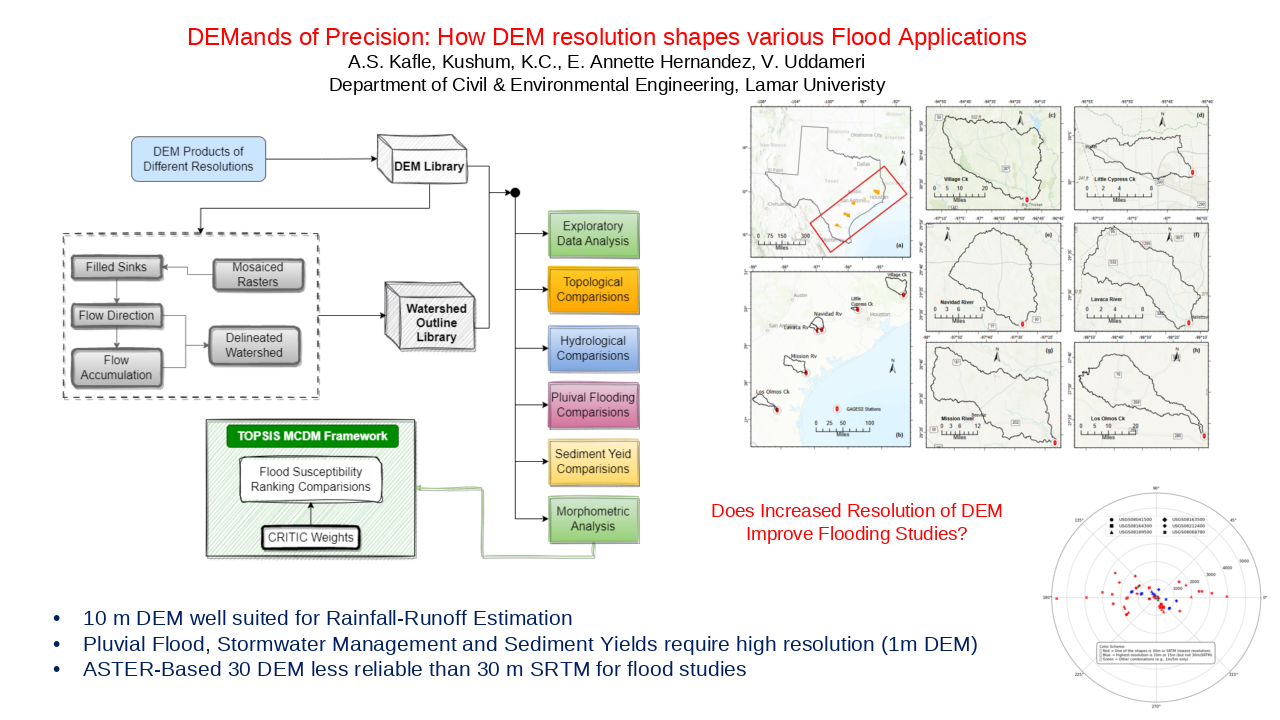
Digital elevation models (DEM) form the backbone of flood related studies. Proper selection of the DEM product is critical to obtain reliable estimates. Most studies aimed at understanding DEM resolution impacts focus on geometric comparisons. A comprehensive structural and functional assessment framework for DEM comparisons is developed here. The structural differences in DEM are used to understand how DEM products produce differing estimates of flooding susceptibility, rainfall-runoff partitioning, sediment flux estimates and impacts of pluvial flooding. While there is no single DEM resolution that is superior, the results indicate that the ASTER-based 30m DEM is generally the least reliable. The widely available 10m 3DEP DEM is well suited for rainfall-runoff partitioning and flood risk and susceptibility mapping applications. Resampling this DEM to 15m resolution yields similar results and can be used in large domain applications. LiDAR based high-resolution DEMs (1m or less resolution) are best suited for pluvial flood delineations and stormwater management. Even 10m DEM is noted to yield inconsistent results. The 30m ASTER-based DEM yields the most conservative estimate of sediment fluxes due to overprediction of slope and altered watershed shape. The high resolution DEM is therefore recommended for this application as well.
Keywords:
flood management
; floodplain delineation
; GIS
; flood risk
; DEM
; pluvial flooding
1. Introduction
Flood risk assessment and stormwater management applications rely heavily on mathematical models to predict the volume, duration and intensity of runoff as well as associated sediment and pollutant loads [1,2,3]. Watershed delineation is an important first step in these modeling studies to describe the drainage area that contributes to flow of water and pollutants following a rainfall event. Accurate delineation of watersheds is therefore critical to study a wide range of flood and stormwater management issues, including but not limited to, flood risk assessments and management [4], non-point source pollution (NPS) control [5], socio-ecological vulnerability studies [6]; climate change impacts [7] and for fostering participatory adaptation and building community resilience [8] and smart growth [9].
Automated watershed delineation has become common in recent years due to availability of software and data [10,11]. The digital elevation model (DEM) is a critical input for delineation of watersheds and computation of other watershed characteristics such as topographic slope which controls the movement of water and pollutants. A variety of DEM products of varying resolution are currently available. Satellite data such as those derived from Shuttle Radar Topographic Mission (SRTM) [12] are used to derive DEM products with resolutions in the range of 10 m to 30 m. More recently, Light Detection and Ranging (LiDAR) data have been demonstrated to be useful to generate high resolution DEMs with resolutions of 1 m or less [13].
High resolution LiDAR-based DEMs have the potential to accurately capture even small flow paths within a watershed. This is particularly advantageous in flat terrains, where water flow is controlled by small topographic differences. However, their use entails higher computational costs. Furthermore, small errors associated with DEM construction can get amplified and lead to incorrect estimation of flow directions and discrepancies in the amount of water, sediments and pollutants that are transported within the watershed. It is difficult to ascertain a priori whether a higher resolution DEM will improve the application of interest. Therefore, many studies have evaluated the impact of DEM resolutions on watershed characteristics and have been summarized in Table 1. The following main insights can be drawn from these studies - 1) DEM resolution plays an important role in flood and stormwater management applications; 2) Higher resolution DEM does not necessarily improve the prediction accuracy; 3) Sediment and nutrient loading estimates are generally more sensitive to DEM resolution compared to flood (water) volumes. 4) DEM resolution impacts decreased with increased topographic relief within the watershed and 5) The noise associated with higher resolution DEM could mask the benefits of accurate delineation and therefore a more coarser DEM could sometimes yield better overall performance.
While these studies offer many useful insights, many were conducted at a time when LiDAR based DEM models were at their infancy. Therefore, recent advancements in LiDAR and satellite technologies and associated processing algorithms have not been fully documented [14]. Similarly, many studies focus on the delineation of the watershed and not the utility of the delineated watershed in flood and stormwater management studies. Also, the role of DEM for pluvial flooding assessments is a burgeoning area of research where the role of DEMs is beginning to be studied especially over large spatial scales [15,16].

Table 1.
Studies focused on the Resolution of DEM on Flood and Stormwater Management Applications.
| Author | References | DEM Res. | Study Area | Key Findings |
|---|---|---|---|---|
| Teegavarapu et al., 2006 | [17] | 10m and 90m | Kentucky River, USA | Finer DEM improved watershed delineation and pollutant-load estimates; coarse grid overstated loads. |
| Wu et al., 2007 | [18] | 30m to 3000 m | Goodwin & Peacheater Creeks, USA | Grid size governs topographic index; coarser DEM smooths terrain, degrading slope and contributing-area estimates. |
| Dixon & Earls, 2009 | [19] | 30 m, 90 m | Charlie Creek, Florida | SWAT hydrographs differed between native and resampled DEMs; resolution change alters predicted flows. |
| Charrier & Li, 2012 | [20] | 1m to 30 m | Camp Creek, Missouri | Resampled 3–5 m LiDAR matched10m DEM; 1 m over-sensitive; coarser USGS DEMs added uncertainty. |
| Zhang et al., 2014 | [21] | 30m to 1000m | Xiangxi River, China | Nutrient and flow outputs highly resolution-sensitive; coarse grids under-predicted transport. |
| Reddy & Reddy, 2015 | [22] | 20m to 1000m | Kaddam, India | Sediment yields more sensitive than runoff; Finer DEM gave best accuracy-effort balance. |
| Tan et al., 2015 | [23] | 20m to 1500m | Johor River, Malaysia | DEM resolution outweighed source influence; coarse cells under-estimated streamflow. |
| Buakhao & Kangrang, 2016 | [24] | 5m to 90m | Chiang Mai, Thailand | Stream length/slope resolution-sensitive; watershed area less so; ASTER DEM accurate. |
| Hamel et al., 2017 | [25] | 10m to 180m | USA, HI, PR, Kenya, Spain | Finer DEMs refined sediment-delivery ratios across diverse terrains. |
| Nagaveni et al., 2019 | [26] | 12m to 90m | Krishna basin, India | Coarse DEMs lost terrain detail and increased runoff error; resolution most influential |
| Roostaee & Deng, 2020 | [27] | 3.5m to 100m | OR, IA, LA (USA) | Flat basins are very sensitive to resolution; drainage area shrinks with coarse DEMs; steep basins little impact. |
| Al-Khafaji et al., 2020 | [28] | 30m to 1000m | Iraqi Watersheds | Higher resolution increased HRU count but did not always improve flow simulation in flat areas. |
| Fan et al., 2021 | [29] | 12.5 m to 1000 m | Northeast China | Runoff depth fell as cell size grew; land-use resolution sometimes dominated influence. No difference for DEM ≤ 100 m. |
| Datta et al., 2022 | [30] | 30m to 225m | Bangladeshi Watersheds | Coarse DEMs inflated areas with less perimeter & shortened streams. |
| Roostaee & Deng, 2023 | [31] | 30m and 100m | IA, LA (USA) | DEM source caused more uncertainty in simulations than resolution; sediment most affected, nitrate least. |
| Choudhary et al., 2025 | [32] | 12.5m to 30m | Rajasthan, India | ALOS PALSAR 12.5 m gave the best flow-path and catchment delineation; DEM choice decisive. |
| Avila-Ruiz et al., 2025 | [33] | 0.13m and 5m | Mexicali, Mexico | Finer DEM greatly improved urban drainage modelling over coarser DEM. |
| Muthusamy et al., 2021 | [34] | 1m to 50m | Cumbria, UK | Coarser DEM inflates flood extent/depth; Hybrid DEM improves accuracy. |
| de Almeida et al., 2018 | [35] | 10cm | Warwickshire, UK | Decimetric terrain changes shifted flood extent, depth, timing; high res needed but computationally heavy. |
| Aristizábal, 2023 | [36] | 3m to 90m | Neuse River, NC | Accuracy declined sharply beyond 60 m; mid-res (~30 m) balanced runtime and reliability. |
| Savage et al., 2016 | [37] | 10m to 50m | Imera basin, Sicily | Resolution chiefly affected local water depth/timing; gains diminished below 10 m. |
| Hsu et al., 2016 | [38] | 1m to 50m | Sanyei, Taiwan | Coarse grids over-predicted inundation by up to 150 %; high res captured bottlenecks. |
| Ozdemir et al., 2013 | [39] | 10cm to 1m | Alcester, UK | 0.10 m DEM captured kerbs/ramps vital for pluvial flows; friction less influential than resolution. |
| Xu et al., 2021 | [40] | 30m and 90m | Yangtze River Delta, China |
High-res DEM improved flow paths and depression mapping in flat terrain, enhancing pluvial models. |
Based on the insights from the literature review and an assessment of critical data gaps, the two main goals of this study are - 1) To evaluate the role of DEM resolution on obtaining flood characteristics, sediment yield estimates, and, mapping the susceptibility of flooding and 2) To investigate the role of DEM resolution on characterizing pluvial flood inundation. As an ancillary goal, the study also presents new topological metrics to capture the differences in watershed delineations obtained using various resolution DEMs. While accomplishing these objectives, the study develops an integrated DEM evaluation framework that proposes several new structural measures to understand geometric differences between DEM products and use these differences to understand the impacts of DEM on various flood related applications. Therefore, the proposed framework is comprehensive and integrates both structural and functional evaluation of DEM products within one integrated scheme. The developed framework generates insights that are directly useful to flood planning and resiliency building efforts. The mathematical framework developed in this study are illustrated using a set of watershed along the Texas Gulf Coast. This region is known for its relatively flat terrains and its high susceptibility to flooding and therefore serves as a useful test-bed to evaluate and illustrate the benefits of the proposed framework.
2. Mathematical Framework
2.1. Exploratory Data Analysis
Consider a set of DEM products that are available within a region (watershed). Exploratory data analysis (EDA) including summary statistics, empirical cumulative distribution functions provide the first cut evaluation of similarities and differences between different DEM products. Despite their qualitative nature, EDA is a crucial first step of the proposed framework to not only gain preliminary insights, but also evaluate the quality of the data of the various DEM products. In addition to summary statistical measures, differences in elevation predictions can also be evaluated by sampling a set of points (within known coordinates) from different DEMs and using both exploratory and confirmatory statistical analysis methods.
2.2. Terrain Based Comparisions
Here, is the DEM pixel area, ∆Z is the elevation difference, d as the horizontal distance between adjacent grid cells, represents all the cells present in the analysis domain with k representing the set of all neighboring upstream cells contributing flow to cell (i, j).
The primary utility of DEMs are to obtain information about the terrain within a region. Changes in terrain have important hydrological implications on the flow of water and transport of sediments and pollutants. Table 2 provides details of the four terrain-based indices that were utilized in this study. Terrain-based analysis are particularly useful to understand the role of pluvial flooding [42]. Therefore, the metrics in Table 2, are useful to evaluate the role of DEM in pluvial flooding studies.
2.3. Topological Comparisons
Watersheds serve as fundamental units for flood management. Topological comparisons help assess the nature and extent to which two watersheds that are delineated using two different DEM products are similar. Table 3 defines the various topological metrics that were utilized in this study. In this study, the D8 algorithm [43] was employed to derive flow direction from the various DEM products. The D8 model was chosen because it is not only computationally efficient, its compatibility with several widely used hydrologic models such as SWAT, HEC-HMS [44,45] that are employed for flood modeling studies. The D8 algorithm is also the basis for improved modeling of human-induced alterations in watersheds [46]. Given the simplicity and ease of use, the D8 algorithm has been recommended as part of open Geospatial Data Software and Standard [47]. Flow accumulation was computed based on the individual flow directions, providing insight into water routing and stream network formation [48,49].
Table 2 lists the various metrics that were identified to quantifying the spatial differences between two (or more) watershed delineations. The metrics are developed by adopting various standard topological indices that have been used in other applications for scientific comparison and visualization [50,51,52]. Together, these metrics provide a structured approach to quantifying spatial differences between watershed delineations, supporting systematic comparison of how DEM resolution influences watershed geometry.
2.4. Flood Susceptibility Ranking Comparisons
While topological and terrain derived comparisons provide useful information on quantifying the differences between two or more DEM products, the real-test of DEMs must focus on the results they provide in different flood related applications. DEM derived information is widely used for mapping flood susceptibility and risk-based ranking of watersheds in regional flood planning studies. Therefore, flood susceptibility mapping was selected as an application to test the impacts of various DEM resolutions.
Watershed morphometric parameters serve as robust indicators for assessing the impacts of DEM resolution on flood risk mapping, as they are closely linked to key hydrologic processes such as runoff, peak flow, lag time, soil erosion, and sediment [53]. These parameters have been extensively applied in flood risk mapping studies, particularly for ungauged watersheds and in screening-level analyses where the goal is to rapidly identify flood-prone areas without the need for complex hydrologic modeling [4,54,55,56,57]. In this study, a suite of 17 morphological metrics was assembled for evaluation purposes, categorized into Linear, Areal, and Relief aspects, as summarized in Table 4 and Supplementary Information S1 [57,58,59,60,61,62,63]. These metrics can be derived from various DEM products in conjunction with other watershed specific information that are tabulated in the literature [64] to evaluate the impacts of DEM resolution on flood susceptibility mapping.
A unified metric called the Morphometic Concordance Index (MCI) was developed to evaluate the overall agreement of morphometric indicators across DEM resolutions. The index sums up the deviations from a reference of all parameters into a single unweighted score. Following the Laplace Principle of insufficient reason, the various metrics are not weighted to avoid decision-maker bias and retain simplicity of interpretation. The MCI score is obtained as follows:
where, X is the morphometric criterion, n is the number of criteria, the subscript R refers to a reference DEM and the lower-case, r refers to a DEM of interest.
To more systematically assess the integrated impact of DEM resolution on watershed morphometric characterization, the Technique for Order Preference by Similarity to Ideal Solution (TOPSIS) was employed within a multi-criteria decision-making (MCDM) framework. TOPSIS, introduced by Hwang and Yoon in 1981, has become one of the most widely used MCDM methods [65,66]. While the criteria ratings of TOPIS are obtained from DEM derived products, the final ranking also depends upon criteria weights. Objective weights are obtained directly from the criteria rankings and are increasingly being recommended for use in flood susceptibility mapping [57]. The CRITIC approach was adopted here because it derives weights by integrating the standard deviation and inter-parameter correlations, emphasizing parameters with substantial discriminative power and minimal redundancy [67]. The TOPSIS technique was applied by assuming various DEM products as alternatives separately at each watershed.
2.5. Pluvial Flood Characterization
DEMs also play a crucial rule in studying pluvial flooding. In particular, depressions in DEMs influence the extent of inundation and surface retention of flood water. For identification of these terrain sinks, DEMs were hydrologically conditioned using a depression-filling algorithm, raising sink cells to the elevation of their lowest neighbor. Sink depth was computed as the difference between the original and filled DEMs using the following raster operation:
where the sink depth at cell i, denote the filled DEM, the original DEM, and represents the set of elevation values of the eight neighboring cells surrounding cell i. The resulting sink depth rasters were used to extract statistical summaries, including minimum, maximum, mean, median, and standard deviation. Additionally, total depression area and cumulative sink volume were calculated by summing the product of sink depth and pixel area across all affected cells.
2.6. Flood-Event Modeling Comparison
Hydraulic designs rely on simulation of runoff corresponding to a critical (design) storm event. The information from the generated outflow hydrograph is used to regulate flows in streams and develop stormwater controls in land development studies. The SCS Curve Number (SCS-CN) technique was adopted in this study [68]. While the curve number (CN) is a function of land use and soil types, several other key parameters such as time to peak, lag time and others depend upon DEM derived parameters such as watershed area, length and slopes. Therefore, different DEM products could yield different estimates of flood characteristics. Mathematical details of SCS-CN technique are well documented in the literature [69] so they are not repeated here in the interest of brevity. SCS-CN was implemented with various DEM products for a selected design storm to evaluate how different products affect runoff corresponding to the same rainfall event.
2.7. Sediment Yield Modeling Comparison
Floods cause a significant movement of sediments, which in turn causes loss of agricultural productivity and transport of pollutants. It is therefore imperative that flood risk assessments also consider this aspect. The Revised Universal Soil Loss Equation (RUSLE) model originally developed by the US Department of Agriculture is widely used for sediment erosion studies [70]. While RUSLE incorporates soil and rainfall characteristics, The slope-length (LS) factor requires estimation of slopes and areas (McRoberts et al., 2002) which are DEM dependent. These factors are manipulated in a highly nonlinear manner to obtain the slope length factor (LS). Therefore, the computation of LS can be highly sensitive to the resolution of the DEM which in turn could critically affect the estimated sediment yield. The RUSLE model is also well documented in the literature and as such its mathematical details are not presented here in the interest of brevity. RUSLE implementation workflows using GIS and remote sensing technologies are presented in the literature and were adopted in this study [72].
The overall framework of analysis is presented in Figure 1. As can be seen, the approach is generic and can be scaled to any number of DEM comparisons. In addition, the approach is also comprehensive in that it not only compares various DEM products but also allows comparison of the outputs they generate for supporting flood studies. The comparison is also multi-dimensional in that the DEM evaluation considers both quantity (flood water) and quality (sediment yield) considerations. Therefore, the proposed framework provides a complete picture on the use of DEM for flood related applications.
3. Illustrative Case Study
The study focuses on the Texas Gulf Coast, a region encompassing over 350 miles of shoreline from the US-Mexico border at Brownsville, TX at the south to Texas-Louisiana border in the northeast. The region is home to major cities and metropolitan areas such as Houston, Corpus Christi, and Beaumont-Port Arthur. The region has several ports, five of which are ranked in the nation’s top 20 on the basis of tonnage and support over $450 billion worth of economic activity within Texas and over $1 trillion in the nation [73,74]. In addition, Texas has the highest number of crude oil refineries in the nation, many of which are located along the Gulf of Mexico [75].
The Gulf of Mexico region of Texas is also a climate hot-spot and climate shifts studied using an ensemble of models indicate a greater propensity of fast-moving tropical storms making landfall along the Texas coast [76]. The Texas coast is also known for its biodiversity and unique ecological habitats [77], wherein the resilience of many small communities relies heavily on ecotourism [78]. The hydro-climatology of the Texas Gulf Coast region also varies from humid conditions towards the northeast to semi-arid conditions in the south and provides a valuable test-bed that is of economic, ecological, and social significance as well has considerable hydrologic heterogeneity.
In the wake of Hurricane Harvey in the year 2017, the state of Texas enacted legislation (Senate Bill 8 or SB8) in the year 2019 to develop state flood plan [79]. The state flood plan is assembled in using a bottoms up planning approach considering different aspects of flooding in the states 15 flood planning zones. The state flood plan seeks to identify and mitigate flood hazards to its population and critical infrastructure. The legislative mandate dictates the use state-of-the-art tools and datasets for understanding floods and mitigating their impacts. Given the important role of DEMs in flood characterization, identifying appropriate resolution of DEMs for various flood related studies and evaluating when and where higher resolution LiDAR based DEM data are required becomes critical [80]. This study directly addresses these practical questions using 6 representative watershed across the Texas Gulf Coast. The locations of these watersheds in Texas are depicted in Figure 2. The watersheds are delineated to a USGS gaging station as their pour point. These stations and the listed watershed areas are summarized in Table 5. All stations are part of the USGS GAGES-II database [81] and are identified as those that have not undergone human disturbances. As such, the selected watersheds highlight the impacts of DEM resolution as the results are not affected by human alterations to the elevations.
3.1. Data Compilation and Processing
Four distinct DEM products were employed as the primary datasets for this study (See Table 6). These included a 1 m LiDAR DEM [82,83,84,85], a 1/3 arc-second (10 m) DEM from the USGS 3DEP program [86], a 1 arc-second (~30 m) DEM from ASTER GDEM v3 [87], and a 1 arc-second (~30 m) DEM from the Shuttle Radar Topographic Mission (SRTM) [88]. The selection of these DEMs were based on their data availability and therefore their widespread use in the United States [89,90,91]. SRTM- and ASTER-derived products also commonly applied worldwide [92,93,94]. Hydrologic modeling studies often resample the DEMs to meet their spatial resolution needs or reduce computational burden. To reflect this practice, the 1 m LiDAR and 10 m DEMs were resampled to 5 m and 15 m resolutions, respectively, using nearest-neighbor interpolation.
Raster DEMs were often provided in small tiles to manage storage and distribution. To ensure seamless coverage for each watershed, these tiles were mosaicked into a single continuous raster dataset. A depression-filling operation was applied to eliminate artificial sinks, followed by the computation of flow direction and flow accumulation to establish hydrologic connectivity.
In this study, the D8 algorithm [43] was employed to derive flow direction from the various DEM products. The D8 model was chosen because it is not only computationally efficient, but its compatibility with several widely used hydrologic models such as SWAT, HEC-HMS [44,45] that are employed for flood modeling studies. The D8 algorithm is also the basis for improved modeling of human-induced alterations in watersheds [46]. Given the simplicity and ease of use, the D8 algorithm has been recommended as part of open Geospatial Data Software and Standard [47]. However, the proposed evaluation framework is agnostic to the algorithms used for processing DEM products to generate flow accumulations, paths and directions.
Watershed boundaries were delineated using ArcGIS Pro [48,49] by snapping pour points to the nearest stream network. Once the delineated watersheds were used to obtain the required geomorphic data from the from the NHDPlus dataset [64]. Pluvial flood characteristics such as sink area estimation were also carried out using ArcGIS Pro GIS software. Given the high data volume exceeding 60,000 LiDAR tiles for some basins, custom automated routines in Python and ArcGIS Pro were developed to streamline the data processing workflows. Custom scripts were developed to implement TOPSIS, SCS-CN and RUSLE analysis as well as compute the geomorphic indicators using Python and R programming languages [95,96].
4. Results and Discussion
4.1. Exploratory Data Analysis
Figure 3 depicts the values of various statistical measures (min, max, mean) and important quantiles (5, 25. 50, 75 and 95 percentiles) for different DEM products across different watersheds. The results indicate that higher resolution DEMs (< 15 m resolution) tend to be more consistent across the watersheds. Slight deviations in minimum elevations in some watersheds (e.g., Lavaca, Navidad, Mission Rivers) were traced to localized sinks caused by interpolation artifacts, which were corrected through sink-filling operations. These corrections were noted to have local impacts and did not affect the summary statistics or the other quantiles. These results however highlight that artificial sinks can pose problems at any resolution and even with widely available datasets such as the USGS 1/3 arc-second product.
The 10 m 1/3 arc-second 3DEP DEM product is widely available in the US and in the absence of any local higher resolution data, this product represents the best resolution for hydrologic studies. As such, this product was used as the reference and other products were compared against using using various goodness of fit measures. To facilitate this comparison, a large sample of points (> 300,000) were randomly selected within each watershed and used to extract elevations from all DEM products.
The data were used to compute various goodness of fit measures. The results in Table 7 indicate that DEM products with resolutions less than 15 m show good agreement with the reference 10 m DEM. While the 15 m DEM has the best error metrics, it is important to keep in mind that this DEM was resampled from the 10 m DEM. The analysis indicates that in the absence of higher resolution data the 10 m DEM should provide elevations comparable to higher resolution DEM models. The result also show that 30 m resolution DEMs exhibit greater deviations from the 10 m product. This result is to be expected because the elevation at a point is averaged over a larger area (pixel size) thus, these models lack the ability to retain local variations. It can also be seen that the 30 m SRTM DEM has better error metrics than the 30 m ASTER product. This result likely stems from the fact that SRTM is radar based and as such is not affected by the presence of cloud cover. On the other hand, ASTER is optical based and the elevation computation is affected to a greater degree by atmospheric interference and incident angle [97].
4.2. Terrain Based Assessment
The slopes, flow accumulation were computed pixel by pixel and extracted using a set of points uniformly spaced across the watershed to evaluate variations in terrain based parameters. As the total wetness index (TWI) incorporates both the slope and flow accumulation, its results are of most interest. Figure 4 depicts the TWI values across the areal extent of the Little Cypress Creek, TX (an illustrative watershed). The results show similar trends across all watersheds and as such are not presented here in the interest of brevity.
The results in Figure 4 indicate that the terrain based characteristics, particularly the total wetness index (TWI) is very sensitive to the resolution of the DEM. In general the accumulated area increases with increasing DEM resolution. This result largely arises because the high resolution DEM capture slopes over smaller areas due to their small pixel sizes, as the resolution increases the slopes are averaged over much larger areas. This averaging reduces the slope values which in turn increase the TWI values (as the slope is in the denominator).
The TWI estimates the tendency of the watershed to retain water. The use of lower resolution DEMs indicate greater retention of water within the watershed and therefore lesser outflows as compared to higher resolution DEM products. Greater retention implies lower discharges and an under-estimation of runoff brought forth by the neglect of micro-relief features that control sheet flows. The large over-estimation also implies that the use of coarser DEMs will significantly over-estimate the inundation areas, infiltration and other watershed losses, likely leading to under-design of storm water capture and treatment structures.
4.3. Topological Comparisons
Watershed Boundary Concordance (WBC) metrics indicate strong agreement among high-resolution DEMs (1-15 m), with most watersheds showing values above 0.92, suggesting minimal topological variation across DEM products (see Figure 5). An exception is Little Cypress Creek, where WBC values decline sharply with coarser resolutions, reflecting the importance of fine-scale data in capturing its complex micro-topographic features. Coarse-resolution DEMs (ASTER and SRTM, both 30 m) consistently yield the lowest WBC values across all watersheds, underscoring their limitations in terrain detail. Notably, despite their shared resolution, SRTM outperforms ASTER which is likely due to its radar-based acquisition method, which is less affected by vegetation and atmospheric interference than ASTER’s optical system.
Figure 6 further supports these findings as watershed centroid discrepancies grow with the inclusion of coarse data (red points), while comparisons involving only high-resolution DEMs (green and blue) exhibit tighter spatial alignment. Additional spatial similarity metrics listed in Table 3 are made available in the Supplementary Information for brevity). These results indicate that the containment hull and inter-boundary distance vary little across resolutions. In contrast, Hausdorff Distance values increase notably with coarse-resolution DEMs (especially ASTER and SRTM), indicating greater divergence at the boundaries for these products. From a hydrological standpoint, the divergence in boundaries obtained at coarser resolution arises due to smoothing out of elevations due to averaging over a larger spatial distance. This in turn could impact the surface runoff characteristics as well as weathering along the hill slopes that impact sediment and pollutant transport.
4.4. Role of DEM in Flood Susceptibility Mapping
The Morphometric Concordance Index (MCI), summarized in Figure 7, provides an overall measure of how well each DEM resolution preserves watershed morphometry. High-resolution DEMs consistently achieved high MCI values (>0.86), with the 15 m DEM showing the closest agreement across all watersheds due to its derivation from the reference dataset. Even in sensitive watersheds like Little Cypress Creek, MCI values for these finer resolutions remained above 0.72. In contrast, ASTER yielded the lowest MCI values across all watersheds, reflecting the cumulative impact of deviations in slope and shape distortions. SRTM shows intermediate performance, it is more stable than ASTER but still less reliable than the resampled high-resolution DEMs.
The TOPSIS-based multi-criteria decision-making analysis was carried out using the results from 10 m DEM (most common) as the ideal reference. Therefore, the results in Figure 8 can be interpreted as how the DEMs perform in ranking flood susceptibility as compared to the 10 m reference DEM. As to be expected the 15 m resampled DEM provided the results closest to the 10 m DEM as it was resampled from it. The 1 m and 5 m DEM also provide similar results due to resampling. They are also fairly close to the 10 m DEM result as compared to the 30 m DEMs. However, there is considerable variability across different watersheds. In general, the deviations are higher in flatter terrains which occur in the southern portions of the study area. The results suggest that resampling of DEM to a slightly coarser resolution often does not affect flood susceptibility mapping and the resampling could reduce the computational burden when mapping flood risks over larger domains. Flood risk maps are also highly susceptible to DEM resolution. Both higher and lower resolution DEMs could map risks differently as compared to the 10 m reference DEM. However, the higher resolution DEMs match the 10 m DEM results more closely than the 30 m DEM and as such their usage is preferred to coarser DEMs in large scale flood susceptibility mapping applications.
4.5. Rainfall-Runoff Modeling Applications
Figure 9 and Figure 10 depict the runoff characteristics (peak volume and time to peak respectively) corresponding to a unit rainfall of 6 hr duration at the selected watersheds. The 30 m SRTM DEM consistently produces the largest peak volume and lowest time to peak estimates. Therefore, this DEM resolution offers the most conservative estimates for estimating runoff and planning flood emergency activities. This result is directly correlated to the fact that the 30 m DEM consistently has the lowest time to peak estimates across all watersheds. The time to peak is proportional to the length of the watershed and inversely proportional to the slope. The coarser resolution SRTM provides the smallest distance and steeper slopes compared to other DEM products. In a similar vein, the SRTM model also provides the larger areas which leads to increases in peak volumes. These results are consistent with the watershed boundary concordance metrics. The noted discrepancies in the centroid and boundary delineations (see Figure 5) with increasing resolution explain the observed hydrological impacts. However, the relationship is not consistent across DEM resolutions. Thus, even while DEM products may provide similar overall metrics like watershed area, they may deviate in terms of the shape and slope factors which are also critical for rainfall-runoff modeling. In general, the higher resolution DEMs (1m and 5m) generally provide the next most conservative runoff estimates. These results indicate that for the purposes of rainfall runoff modeling a coarser but reliable DEM such as the 30 m SRTM could perhaps be sufficient for obtaining runoff estimation for flood planning purposes.
4.6. DEM Impacts on Sediment Yield Computations
While the sediment flux estimates vary among different watersheds due to their size and soil characteristics, a consistent pattern can be seen with regards to the DEM products evaluated. The ASTER based 309 m DEM provides the most conservative estimate. The highest resolution DEM (1 m LiDAR) provides the next most conservative estimate. The two DEM factors of interest in the implementation of the RUSLE model are the slope and flow accumulation which are used to obtain the LS factor. As discussed previously, coarser resolution models tend to over-predict the flow accumulation which affects the sediment flux (ceteris paribus). An over-estimation of steepness further increases the flux estimate. These two factors act in consort and cause a very high estimate of sediment flux for ASTER. These two factors are not as fully in consort for the 30 m ASTER and 1 m DEM which tempers their estimates. Again, the relationship between DEM resolution and sediment yield estimates is not consistent and sediment fluxes not only are influenced by the resolution of the DEM but also the method of data collection. It is therefore recommended that multiple DEMs be used to obtain potential ranges of sediment fluxes when applying RUSLE model in flat terrains such as the study area here.
4.7. Role of DEMs in Pluvial Flooding Characterization
Depressions and Sinks cause water to accumulate on relatively impervious surfaces and lead to nuisance issues. Therefore, accurate delineation of depressions and sinks is critical in pluvial flooding studies. Table 8 presents sink depths (relative to the nearest minimum elevation) as well as total sink areas and volumes in selected watersheds. The results highlight the importance of higher resolution DEMs, particularly the 1 m DEM. The coarse resolution DEMs particularly the ASTER based 30 m product appears to result in unrealistic sinks depths and volumes. Again, no consistent pattern can be seen with resolution. Even the widely available 10 m DEM can lead to highly unrealistic values in some watersheds. The highest resolution DEMs (1m) appear to produce consistent results across all watersheds as it captures micro features (depressions, low lying areas) that lead to water accumulations. Therefore, the use of 1m DEM or higher resolution (if available) is recommended here for pluvial flooding studies.
5. Summary and Conclusions
The overall goal of this study was to evaluate the role of DEM resolution on flood characterization. Most previous studies that solely focus on structural evaluation of various DEM products, the present study presents a comprehensive evaluation by integrating structural (topological) comparisons with that across various flood characterization applications. Specifically, the study evaluates the role of DEM resolution and various DEM products for - 1) Mapping flood risks and susceptibility; 2) Estimating runoff associated with a storm event; 3) quantify how DEMs influence sediment fluxes associated with flooding events and 4) the role of DEMs in describing pluvial flooding impacts.
As noted in the literature, there is no one single DEM resolution that is superior across all flood related applications, and this study corroborates this finding as well. However, the study sheds some useful insights related to the selection of DEM products for a given application. The coarser DEMs tend to over-estimate slopes and alter the shape of the watershed (even when they preserve area). These changes are critical for sediment flux estimates as well as rainfall runoff modeling. For rainfall-runoff modeling, the widely available 10 m DEM provides reasonably conservative estimates and the lack of higher resolution DEMs should not impact flood planning studies. In a similar vein, this resolution is also suitable for watershed scale flood susceptibility mapping applications that utilize geomorphological factors. The 10 m DEM can be further resampled to 15 m resolution to reduce computational burden when dealing with large areas. The ASTER based DEM is generally inferior to the radar based (SRTM) DEM at the 30 m resolution. While ASTER provides the most conservative estimate of sediment fluxes, it is very likely that there is significant over-estimation. The ASTER based DEM is generally unsuited for delineating sinks and depressions which are critical to study pluvial flooding. Even the 10 m DEM could be insufficient for this flooding application. Therefore, LiDAR based 1 m DEM products are recommended for these studies. These insights should be useful to flood planners and modelers and help select an appropriate DEM product for their application.
Supplementary Materials
The following supporting information can be downloaded at the website of this paper posted on Preprints.org.
Author Contributions
Conceptualization, VU. and AH; methodology, VU, EH.; software, AK; validation, KC., AH. and VU.; formal analysis, AK.; investigation, AK.; resources, VU; data curation, KC and AK.; writing—original draft preparation, VU.; writing—review and editing, AK, AH.; visualization, AK.; supervision, VU, AH.; project administration, AH, VU; funding acquisition, VU All authors have read and agreed to the published version of the manuscript.
Funding
This research received no external funding.
Data Availability Statement
The raw data that are analyzed in the manuscript are readily available at https://data.tnris.org/ (TxGIO DataHub) and https://doi.org/10.3133/ofr20191096 (NHDPlus High Resolution Dataset). The data presented in this study are available on request from the corresponding author.
Acknowledgments
The authors thank the Graduate Assistantship provided to the first and second authors during the period of this study.
Conflicts of Interest
The authors declare no conflicts of interest.
Abbreviations
The following abbreviations are used in this manuscript:
| DEM | Digital Elevation Model |
| MCDM | Multi Criteria Decision Making |
| TOPSIS | Technique for Order Preference by Similarity to Ideal Solution |
| LiDAR | Light Detection and Ranging |
| NPS | Non-Point Source |
| WBC | Watershed Boundary Concordance |
| SCS-CN | Soil Conservation Service-Curve Number |
| RUSLE | Revised Universal Soil Loss Equation |
| USGS | United States Geological Survey |
| NHD | National Hydrography Dataset |
| SRTM | Shuttle Radar Topography Mission |
| ASTER | Advanced Spaceborne Thermal Emission and Reflection Radiometer |
| SWAT | Soil and Water Assessment Tool |
| HEC-HMS | Hydrologic Engineering Center - Hydrologic Modeling System |
| FEMA | Federal Emergency Management Agency |
References
- Cardoso, M.A.; Almeida, M.C.; Brito, R.S.; Gomes, J.L.; Beceiro, P.; Oliveira, A. 1D/2D Stormwater Modelling to Support Urban Flood Risk Management in Estuarine Areas: Hazard Assessment in the Dafundo Case Study. J Flood Risk Manag 2020, 13, e12663. [Google Scholar] [CrossRef]
- Shen, Y.; Jiang, C. A Comprehensive Review of Watershed Flood Simulation Model. Natural Hazards 2023, 118, 875–902. [Google Scholar] [CrossRef]
- Kumar, V.; Sharma, K.V.; Caloiero, T.; Mehta, D.J.; Singh, K. Comprehensive Overview of Flood Modeling Approaches: A Review of Recent Advances. Hydrology 2023, 10, 141. [Google Scholar] [CrossRef]
- Obeidat, M.; Awawdeh, M.; Al-Hantouli, F. Morphometric Analysis and Prioritisation of Watersheds for Flood Risk Management in Wadi Easal Basin (WEB), Jordan, Using Geospatial Technologies. J Flood Risk Manag 2021, 14, e12711. [Google Scholar] [CrossRef]
- Srinivas, R.; Singh, A.P.; Dhadse, K.; Garg, C. An Evidence Based Integrated Watershed Modelling System to Assess the Impact of Non-Point Source Pollution in the Riverine Ecosystem. J Clean Prod 2020, 246, 118963. [Google Scholar] [CrossRef]
- Cheng, C. EcoWisdom for Climate Justice Planning: Social-Ecological Vulnerability Assessment in Boston’s Charles River Watershed. In Ecological wisdom: Theory and practice; Springer, 2019; pp. 249–265.
- Marin, M.; Clinciu, I.; Tudose, N.C.; Ungurean, C.; Adorjani, A.; Mihalache, A.L.; Davidescu, A.A.; Davidescu, Șerban O.; Dinca, L.; Cacovean, H. Assessing the Vulnerability of Water Resources in the Context of Climate Changes in a Small Forested Watershed Using SWAT: A Review. Environ Res 2020, 184, 109330. [Google Scholar] [CrossRef] [PubMed]
- Balsas, C.J.L. Retaining Social and Cultural Sustainability in the Hudson River Watershed of New York, USA, a Place-Based Participatory Action Research Study. Journal of Place Management and Development 2022, 15, 336–354. [Google Scholar] [CrossRef]
- Weil, K.K.; Cronan, C.S.; Lilieholm, R.J.; Danielson, T.J.; Tsomides, L. A Statistical Analysis of Watershed Spatial Characteristics That Affect Stream Responses to Urbanization in Maine, USA. Applied Geography 2019, 105, 37–46. [Google Scholar] [CrossRef]
- David, S.R.; Murphy, B.P.; Czuba, J.A.; Ahammad, M.; Belmont, P. USUAL Watershed Tools: A New Geospatial Toolkit for Hydro-Geomorphic Delineation. Environmental Modelling & Software 2023, 159, 105576. [Google Scholar] [CrossRef]
- Baker, M.E.; Weller, D.E.; Jordan, T.E. Comparison of Automated Watershed Delineations. Photogramm Eng Remote Sensing 2006, 72, 159–168. [Google Scholar] [CrossRef]
- Yang, L.; Meng, X.; Zhang, X. SRTM DEM and Its Application Advances. Int J Remote Sens 2011, 32, 3875–3896. [Google Scholar] [CrossRef]
- Muhadi, N.A.; Abdullah, A.F.; Bejo, S.K.; Mahadi, M.R.; Mijic, A. The Use of LiDAR-Derived DEM in Flood Applications: A Review. Remote Sens (Basel) 2020, 12, 2308. [Google Scholar] [CrossRef]
- Kubendiran, I.; Ramaiah, M. Modeling, Mapping and Analysis of Floods Using Optical, Lidar and SAR Datasets—a Review. Water Resources 2024, 51, 438–448. [Google Scholar] [CrossRef]
- Huang, H.; Liao, W.; Lei, X.; Wang, C.; Cai, Z.; Wang, H. An Urban DEM Reconstruction Method Based on Multisource Data Fusion for Urban Pluvial Flooding Simulation. J Hydrol (Amst) 2023, 617, 128825. [Google Scholar] [CrossRef]
- Samadi, A.; Jafarzadegan, K.; Moradkhani, H. DEM-Based Pluvial Flood Inundation Modeling at a Metropolitan Scale. Environmental Modelling & Software 2025, 183, 106226. [Google Scholar] [CrossRef]
- Teegavarapu, R.S. V; Viswanathan, C.; Ormsbee, L. Effect of Digital Elevation Model (DEM) Resolution on the Hydrological and Water Quality Modeling. In Proceedings of the World Environmental and Water Resource Congress 2006: Examining the Confluence of Environmental and Water Concerns; 2006; pp. 1–8. [Google Scholar]
- Wu, S.; Li, J.; Huang, G.H. Modeling the Effects of Elevation Data Resolution on the Performance of Topography-Based Watershed Runoff Simulation. Environmental Modelling & Software 2007, 22, 1250–1260. [Google Scholar] [CrossRef]
- Dixon, B.; Earls, J. Resample or Not?! Effects of Resolution of DEMs in Watershed Modeling. Hydrological Processes: An International Journal 2009, 23, 1714–1724. [Google Scholar] [CrossRef]
- Charrier, R.; Li, Y. Assessing Resolution and Source Effects of Digital Elevation Models on Automated Floodplain Delineation: A Case Study from the Camp Creek Watershed, Missouri. Applied Geography 2012, 34, 38–46. [Google Scholar] [CrossRef]
- Zhang, P.; Liu, R.; Bao, Y.; Wang, J.; Yu, W.; Shen, Z. Uncertainty of SWAT Model at Different DEM Resolutions in a Large Mountainous Watershed. Water Res 2014, 53, 132–144. [Google Scholar] [CrossRef] [PubMed]
- Reddy, A.S.; Reddy, M.J. Evaluating the Influence of Spatial Resolutions of DEM on Watershed Runoff and Sediment Yield Using SWAT. Journal of Earth System Science 2015, 124, 1517–1529. [Google Scholar] [CrossRef]
- Tan, M.L.; Ficklin, D.L.; Dixon, B.; Yusop, Z.; Chaplot, V. Impacts of DEM Resolution, Source, and Resampling Technique on SWAT-Simulated Streamflow. Applied Geography 2015, 63, 357–368. [Google Scholar] [CrossRef]
- Buakhao, W.; Kangrang, A. DEM Resolution Impact on the Estimation of the Physical Characteristics of Watersheds by Using SWAT. Advances in Civil Engineering 2016, 2016. [Google Scholar] [CrossRef]
- Hamel, P.; Falinski, K.; Sharp, R.; Auerbach, D.A.; Sánchez-Canales, M.; Dennedy-Frank, P.J. Sediment Delivery Modeling in Practice: Comparing the Effects of Watershed Characteristics and Data Resolution across Hydroclimatic Regions. Science of the Total Environment 2017, 580, 1381–1388. [Google Scholar] [CrossRef] [PubMed]
- Nagaveni, C.; Kumar, K.P.; Ravibabu, M.V. Evaluation of TanDEMx and SRTM DEM on Watershed Simulated Runoff Estimation. Journal of Earth System Science 2019, 128, 1–11. [Google Scholar] [CrossRef]
- Roostaee, M.; Deng, Z. Effects of Digital Elevation Model Resolution on Watershed-Based Hydrologic Simulation. Water Resources Management 2020, 34, 2433–2447. [Google Scholar] [CrossRef]
- Al-Khafaji, M.; Saeed, F.H.; Al-Ansari, N. The Interactive Impact of Land Cover and DEM Resolution on the Accuracy of Computed Streamflow Using the SWAT Model. Water Air Soil Pollut 2020, 231, 416. [Google Scholar] [CrossRef]
- Fan, J.; Galoie, M.; Motamedi, A.; Huang, J. Assessment of Land Cover Resolution Impact on Flood Modeling Uncertainty. Hydrology Research 2021, 52, 78–90. [Google Scholar] [CrossRef]
- Datta, S.; Karmakar, S.; Mezbahuddin, S.; Hossain, M.M.; Chaudhary, B.S.; Hoque, M.E.; Abdullah Al Mamun, M.M.; Baul, T.K. The Limits of Watershed Delineation: Implications of Different DEMs, DEM Resolutions, and Area Threshold Values. Hydrology Research 2022, 53, 1047–1062. [Google Scholar] [CrossRef]
- Roostaee, M.; Deng, Z. Effects of Digital Elevation Model Data Source on HSPF-Based Watershed-Scale Flow and Water Quality Simulations. Environmental Science and Pollution Research 2023, 30, 31935–31953. [Google Scholar] [CrossRef] [PubMed]
- Choudhary, R.; Munoth, P.; Goyal, R. Comparative Analysis of Digital Elevation Models for Assessing. Hydrology and Hydrologic Modelling: Proceedings of HYDRO 2023 2025, 410, 219. [Google Scholar]
- Avila-Ruiz, W.; Salazar-Briones, C.; Ruiz-Gibert, J.M.; Lomelí-Banda, M.A.; Saiz-Rodríguez, J.A. Comparison of High-Resolution Digital Elevation Models for Customizing Hydrological Analysis of Urban Basins: Considerations, Opportunities, and Implications for Stormwater System Design. CivilEng 2025, 6, 8. [Google Scholar] [CrossRef]
- Muthusamy, M.; Casado, M.R.; Butler, D.; Leinster, P. Understanding the Effects of Digital Elevation Model Resolution in Urban Fluvial Flood Modelling. J Hydrol (Amst) 2021, 596, 126088. [Google Scholar] [CrossRef]
- de Almeida, G.A.M.; Bates, P.; Ozdemir, H. Modelling Urban Floods at Submetre Resolution: Challenges or Opportunities for Flood Risk Management? J Flood Risk Manag 2018, 11, S855–S865. [Google Scholar] [CrossRef]
- Aristizábal, F. High Resolution Flood Inundation Mapping From Remote Sensing Observations and Hydrology Models at Continental Scales; University of Florida, 2023; ISBN 9798380609128.
- Thomas Steven Savage, J.; Pianosi, F.; Bates, P.; Freer, J.; Wagener, T. Quantifying the Importance of Spatial Resolution and Other Factors through Global Sensitivity Analysis of a Flood Inundation Model. Water Resour Res 2016, 52, 9146–9163. [Google Scholar] [CrossRef]
- Hsu, Y.-C.; Prinsen, G.; Bouaziz, L.; Lin, Y.-J.; Dahm, R. An Investigation of DEM Resolution Influence on Flood Inundation Simulation. Procedia Eng 2016, 154, 826–834. [Google Scholar] [CrossRef]
- Ozdemir, H.; Sampson, C.C.; de Almeida, G.A.M.; Bates, P.D. Evaluating Scale and Roughness Effects in Urban Flood Modelling Using Terrestrial LIDAR Data. Hydrol Earth Syst Sci 2013, 17, 4015–4030. [Google Scholar] [CrossRef]
- Xu, K.; Fang, J.; Fang, Y.; Sun, Q.; Wu, C.; Liu, M. The Importance of Digital Elevation Model Selection in Flood Simulation and a Proposed Method to Reduce DEM Errors: A Case Study in Shanghai. International Journal of Disaster Risk Science 2021, 12, 890–902. [Google Scholar] [CrossRef]
- Beven, K.J.; Kirkby, M.J. A Physically Based, Variable Contributing Area Model of Basin Hydrology/Un Modèle à Base Physique de Zone d’appel Variable de l’hydrologie Du Bassin Versant. Hydrological sciences journal 1979, 24, 43–69. [Google Scholar] [CrossRef]
- Zhang, X.; Kang, A.; Ye, M.; Song, Q.; Lei, X.; Wang, H. Influence of Terrain Factors on Urban Pluvial Flooding Characteristics: A Case Study of a Small Watershed in Guangzhou, China. Water (Basel) 2023, 15, 2261. [Google Scholar] [CrossRef]
- O’Callaghan, J.F.; Mark, D.M. The Extraction of Drainage Networks from Digital Elevation Data. Comput Vis Graph Image Process 1984, 28, 323–344. [Google Scholar] [CrossRef]
- Wu, M.; Shi, P.; Chen, A.; Shen, C.; Wang, P. Impacts of DEM Resolution and Area Threshold Value Uncertainty on the Drainage Network Derived Using SWAT. Water Sa 2017, 43, 450–462. [Google Scholar] [CrossRef]
- Barbosa, J.H.S.; Fernandes, A.; Lima, A.; Assis, L. The Influence of Spatial Discretization on HEC-HMS Modelling: A Case Study. International Journal of Hydrology 2019, 3, 442–449. [Google Scholar] [CrossRef]
- Sun, C.; Chen, L.; Liu, H.B.; Zhu, H.; Lü, M.Q.; Chen, S.B.; Wang, Y.W.; Shen, Z.Y. New Modeling Framework for Describing the Pollutant Transport and Removal of Ditch-pond System in an Agricultural Catchment. Water Resour Res 2021, 57, e2021WR031077. [Google Scholar] [CrossRef]
- Sit, M.; Sermet, Y.; Demir, I. Optimized Watershed Delineation Library for Server-Side and Client-Side Web Applications. Open Geospatial Data, Software and Standards 2019, 4, 8. [Google Scholar] [CrossRef]
- Djokic, D. Arc Hydro in ArcGIS Pro: The Next Generation of Tools for Water Resources. In Proceedings of the Esri Federal GIS Conference Proceedings; 2020. [Google Scholar]
- ESRI Inc. ArcGIS Pro 2022.
- Capozziello, S.; De Falco, V.; Ferrara, C. Comparing Equivalent Gravities: Common Features and Differences. The European Physical Journal C 2022, 82, 865. [Google Scholar] [CrossRef]
- Yan, L.; Masood, T. Bin; Sridharamurthy, R.; Rasheed, F.; Natarajan, V.; Hotz, I.; Wang, B. Scalar Field Comparison with Topological Descriptors: Properties and Applications for Scientific Visualization. In Proceedings of the Computer Graphics Forum; Wiley Online Library, 2021; Vol. 40; pp. 599–633. [Google Scholar] [CrossRef]
- Ali, M.; Hussain, Z.; Yang, M.-S. Hausdorff Distance and Similarity Measures for Single-Valued Neutrosophic Sets with Application in Multi-Criteria Decision Making. Electronics (Basel) 2022, 12, 201. [Google Scholar] [CrossRef]
- Sarkar, P.; Kumar, P.; Vishwakarma, D.K.; Ashok, A.; Elbeltagi, A.; Gupta, S.; Kuriqi, A. Watershed Prioritization Using Morphometric Analysis by MCDM Approaches. Ecol Inform 2022, 70, 101763. [Google Scholar] [CrossRef]
- Bhat, M.S.; Alam, A.; Ahmad, S.; Farooq, H.; Ahmad, B. Flood Hazard Assessment of Upper Jhelum Basin Using Morphometric Parameters. Environ Earth Sci 2019, 78, 1–17. [Google Scholar] [CrossRef]
- Bhattacharya, J.P.; Howell, C.D.; MacEachern, J.A.; Walsh, J.P. Bioturbation, Sedimentation Rates, and Preservation of Flood Events in Deltas. Palaeogeogr Palaeoclimatol Palaeoecol 2020, 560, 110049. [Google Scholar] [CrossRef]
- Topno, A.R.; Job, M.; Rusia, D.K.; Kumar, V.; Bharti, B.; Singh, S.D. Prioritization and Identification of Vulnerable Sub-Watersheds Using Morphometric Analysis and an Integrated AHP-VIKOR Method. Water Supply 2022, 22, 8050–8064. [Google Scholar] [CrossRef]
- Mahmoodi, E.; Azari, M.; Dastorani, M.T. Comparison of Different Objective Weighting Methods in a Multi-criteria Model for Watershed Prioritization for Flood Risk Assessment Using Morphometric Analysis. J Flood Risk Manag 2023, 16, e12894. [Google Scholar] [CrossRef]
- Lalduhawma, K.; Rao, K.S.; Rao, U.B. GIS-Based Morphometric Analysis of Sub-Watersheds at Tut River Basin, Mizoram. In Proceedings of the Mizoram Science Congress 2018 (MSC 2018); Atlantis Press; 2018; pp. 87–93. [Google Scholar]
- Smith, K.G. Standards for Grading Texture of Erosional Topography. Am J Sci 1950, 248, 655–668. [Google Scholar] [CrossRef]
- Miller, V.C. A Quantitative Geomorphic Study of Drainage Basin Characteristics in the Clinch Mountain Area Virginia and Tennessee (Proj. NR 389–402, Technical Report 3). New York, NY: Department of Geology, ONR, Columbia University, Virginia and Tennessee. Accession Number: AD0057755 1953.
- Horton, R.E. Drainage-Basin Characteristics. Transactions, American geophysical union 1932, 13, 350–361. [Google Scholar]
- Schumm, S.A. Evolution of Drainage Systems and Slopes in Badlands at Perth Amboy, New Jersey. Geol Soc Am Bull 1956, 67, 597–646. [Google Scholar] [CrossRef]
- Horton, R.E. Erosional Development of Streams and Their Drainage Basins; Hydrophysical Approach to Quantitative Morphology. Geol Soc Am Bull 1945, 56, 275–370. [Google Scholar] [CrossRef]
- U.S. Geological Survey National Hydrography Dataset Plus (NHDPlus). 2023.
- Tzeng, G.-H.; Huang, J.-J. Multiple Attribute Decision Making: Methods and Applications; CRC press, 2011; ISBN 1439861579.
- Chakraborty, S. TOPSIS and Modified TOPSIS: A Comparative Analysis. Decision Analytics Journal 2022, 2, 100021. [Google Scholar] [CrossRef]
- Diakoulaki, D.; Mavrotas, G.; Papayannakis, L. Determining Objective Weights in Multiple Criteria Problems: The Critic Method. Comput Oper Res 1995, 22, 763–770. [Google Scholar] [CrossRef]
- Mishra, S.K.; Singh, V.P.; Mishra, S.K.; Singh, V.P. SCS-CN Method. Soil conservation service curve number (SCS-CN) methodology 2003, 84–146.
- Cronshey, R. Urban Hydrology for Small Watersheds; US Department of Agriculture, Soil Conservation Service, Engineering Division, 1986.
- Kumar, M.; Sahu, A.P.; Sahoo, N.; Dash, S.S.; Raul, S.K.; Panigrahi, B. Global-Scale Application of the RUSLE Model: A Comprehensive Review. Hydrological Sciences Journal 2022, 67, 806–830. [Google Scholar] [CrossRef]
- McRoberts, R.E.; Nelson, M.D.; Wendt, D.G. Stratified Estimation of Forest Area Using Satellite Imagery, Inventory Data, and the k-Nearest Neighbors Technique. Remote Sens Environ 2002, 82, 457–468. [Google Scholar] [CrossRef]
- Fahd, S.; Waqas, M.; Zafar, Z.; Soufan, W.; Almutairi, K.F.; Tariq, A. Integration of RUSLE Model with Remotely Sensed Data over Google Earth Engine to Evaluate Soil Erosion in Central Indus Basin. Earth Surf Process Landf 2025, 50, e70019. [Google Scholar] [CrossRef]
- TXDOT Historic Funding Approved for Texas Seaports. TXDOT Newsroom 2023.
- USDOT 2023 Port Performance Freight Statistics Program: Annual Report to Congress. 2023. [CrossRef]
- U.S. EIA Texas State Energy Profile; 2024.
- Hassanzadeh, P.; Lee, C.-Y.; Nabizadeh, E.; Camargo, S.J.; Ma, D.; Yeung, L.Y. Effects of Climate Change on the Movement of Future Landfalling Texas Tropical Cyclones. Nat Commun 2020, 11, 3319. [Google Scholar] [CrossRef] [PubMed]
- Thorhaug, A.L.; Poulos, H.M.; López-Portillo, J.; Barr, J.; Lara-Domínguez, A.L.; Ku, T.C.; Berlyn, G.P. Gulf of Mexico Estuarine Blue Carbon Stock, Extent and Flux: Mangroves, Marshes, and Seagrasses: A North American Hotspot. Science of the total environment 2019, 653, 1253–1261. [Google Scholar] [CrossRef] [PubMed]
- Dunning, K.H. Building Resilience to Natural Hazards through Coastal Governance: A Case Study of Hurricane Harvey Recovery in Gulf of Mexico Communities. Ecological Economics 2020, 176, 106759. [Google Scholar] [CrossRef]
- Perry; Alvarado; Bettencourt; Birdwell; Buckingham; Campbell; Creighton; Fallon; Flores; Hall et. al. 86(R) Senate Bill 8 - An Act Relating to State and Regional Flood Planning; 2019.
- TWDB 2024 State Flood Plan; 2024.
- Falcone, J.A. GAGES-II: Geospatial Attributes of Gages for Evaluating Streamflow; US Geological Survey, 2011.
- USGS Neches River Basin Lidar; 2017; Available at https://data.tnris.org/.
- USGS South Central Texas Lidar; 2018; Available at https://data.tnris.org/.
- USGS Hurricane Lidar; 2019; Available at https://data.tnris.org/.
- USGS South Texas Lidar; 2018; Available at https://data.tnris.org/.
- USGS USGS 3D Elevation Program Digital Elevation Model; 2019; Available for Texas at https://data.tnris.org/.
- NASA, M. AIST, Japan Spacesystems and US/Japan ASTER Science Team: ASTER Global Digital Elevation Model V003, NASA EOSDIS Land Processes DAAC [Data Set] 2019.
- Hennig, T.A.; Kretsch, J.L.; Pessagno, C.J.; Salamonowicz, P.H.; Stein, W.L. The Shuttle Radar Topography Mission. In Proceedings of the Digital Earth Moving: First International Symposium, DEM 2001 Manno, Switzerland, 2001, September 5–7 2001; Proceedings; Springer. pp. 65–77. [Google Scholar]
- Zhang, C.; Su, H.; Li, T.; Liu, W.; Mitsova, D.; Nagarajan, S.; Teegavarapu, R.; Xie, Z.; Bloetscher, F.; Yong, Y. Modeling and Mapping High Water Table for a Coastal Region in Florida Using Lidar DEM Data. Groundwater 2021, 59, 190–198. [Google Scholar] [CrossRef] [PubMed]
- Gesch, D.B.; Oimoen, M.J.; Evans, G.A. Accuracy Assessment of the US Geological Survey National Elevation Dataset, and Comparison with Other Large-Area Elevation Datasets: SRTM and ASTER; US Geological Survey, 2014.
- Witt III, E.C. Evaluation of the US Geological Survey Standard Elevation Products in a Two-Dimensional Hydraulic Modeling Application for a Low Relief Coastal Floodplain. J Hydrol (Amst) 2015, 531, 759–767. [Google Scholar] [CrossRef]
- Simard, M.; Denbina, M.; Marshak, C.; Neumann, M. A Global Evaluation of Radar-derived Digital Elevation Models: SRTM, NASADEM, and GLO-30. J Geophys Res Biogeosci 2024, 129, e2023JG007672. [Google Scholar] [CrossRef]
- Huang, J.; Yu, Y. Vertical Accuracy Assessment of the ASTER, SRTM, GLO-30, and ATLAS in a Forested Environment. Forests 2024, 15, 426. [Google Scholar] [CrossRef]
- Uuemaa, E.; Ahi, S.; Montibeller, B.; Muru, M.; Kmoch, A. Vertical Accuracy of Freely Available Global Digital Elevation Models (ASTER, AW3D30, MERIT, TanDEM-X, SRTM, and NASADEM). Remote Sens (Basel) 2020, 12, 3482. [Google Scholar] [CrossRef]
- Python Software Foundation Python Version 3.11.9 2024.
- R Core Team R Language Definition. Vienna, Austria: R foundation for statistical computing 2000, 3, 116.
- Han, H.; Zeng, Q.; Jiao, J. Quality Assessment of TanDEM-X DEMs, SRTM and ASTER GDEM on Selected Chinese Sites. Remote Sens (Basel) 2021, 13, 1304. [Google Scholar] [CrossRef]
Figure 1.
Workflow for Comprehensive DEM Analysis.
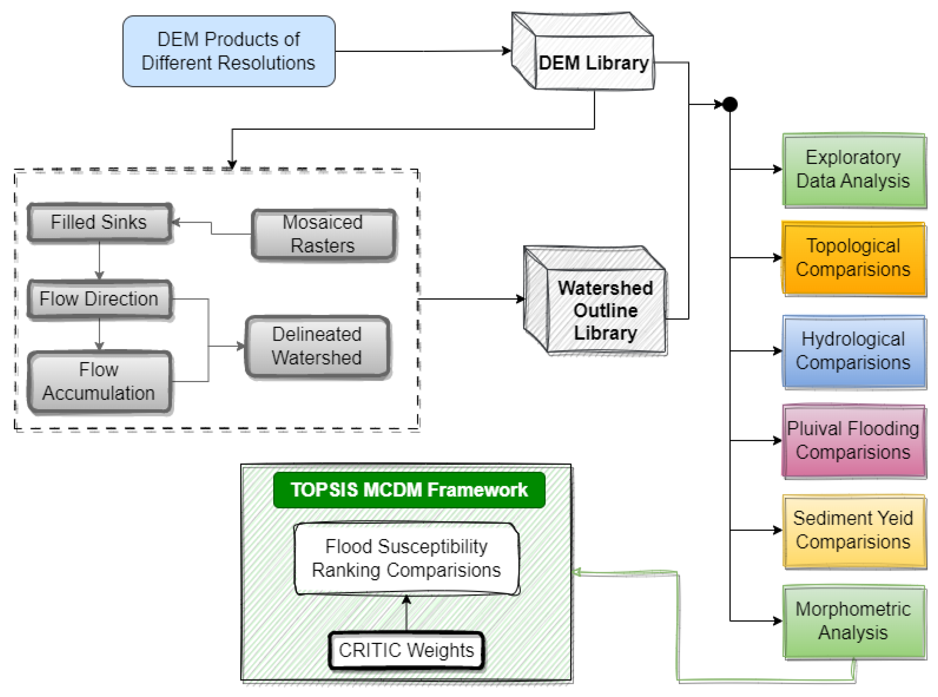
Figure 2.
(a) Study Area; (b) The selected Watersheds; (c) Village Creek Watershed; (d) Little Cypress Creek Watershed; (e) Navidad River Watershed; (f) Lavaca River Watershed; (g) Mission River Watershed and (h) Los Olmos Creek Watershed.
Figure 2.
(a) Study Area; (b) The selected Watersheds; (c) Village Creek Watershed; (d) Little Cypress Creek Watershed; (e) Navidad River Watershed; (f) Lavaca River Watershed; (g) Mission River Watershed and (h) Los Olmos Creek Watershed.
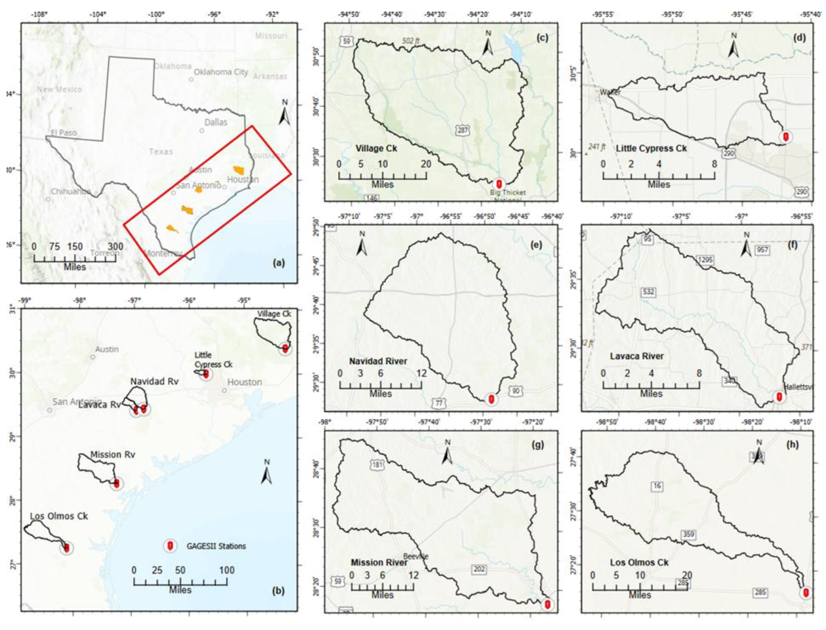
Figure 3.
Comparison of Elevations Across Various Quantiles.
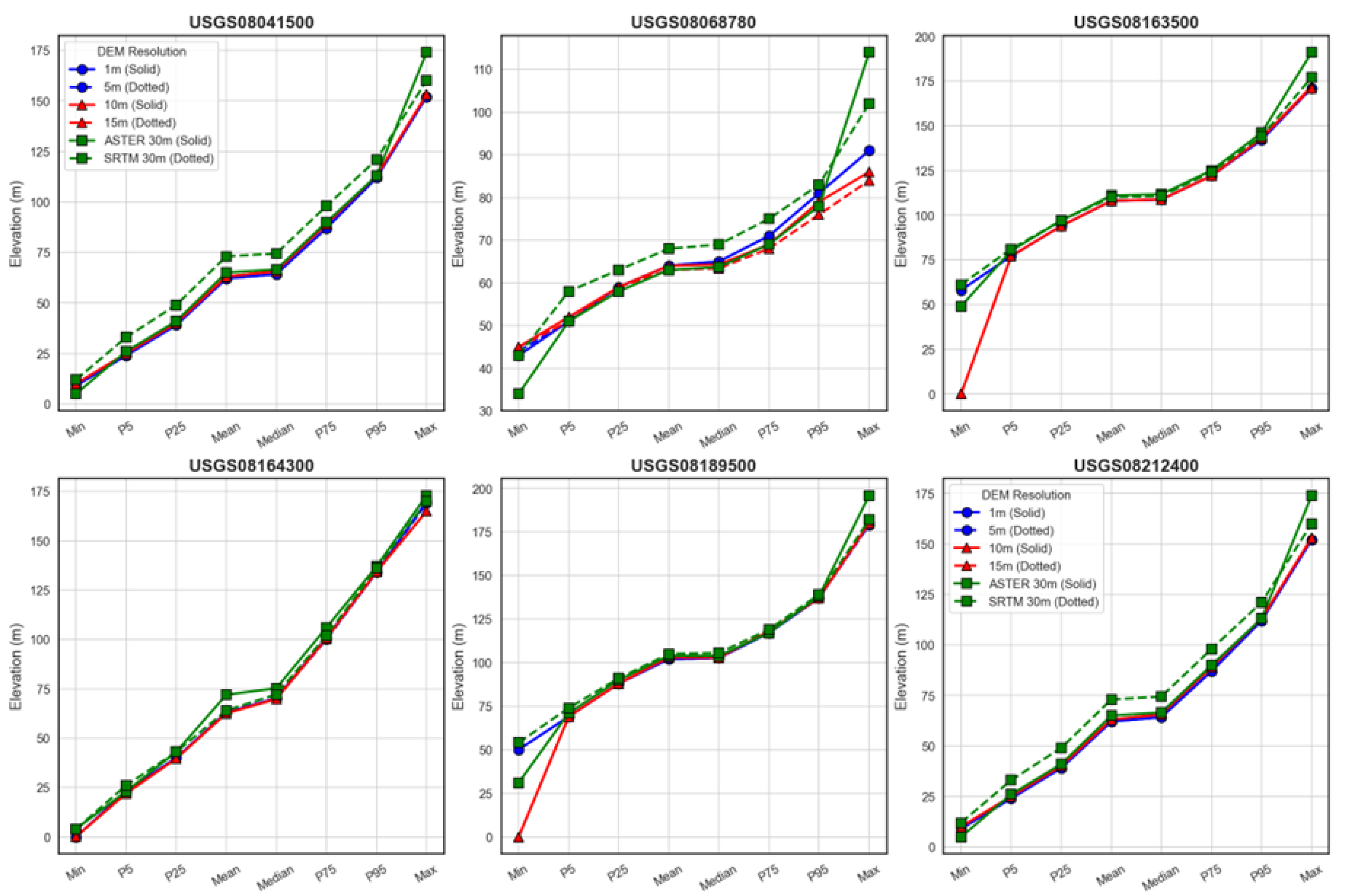
Figure 4.
Comparison of TWI for various DEM Resolutions across Little Cypress Creek, TX.
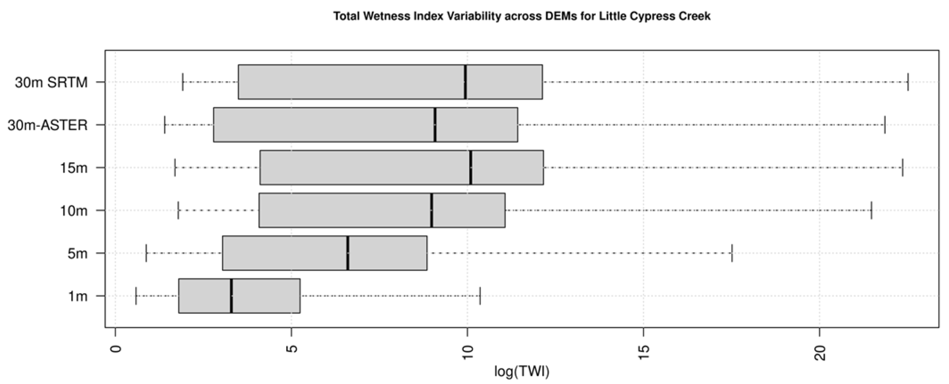
Figure 5.
Watershed Boundary Concordance (WBC) metrics across all watersheds and resolutions.
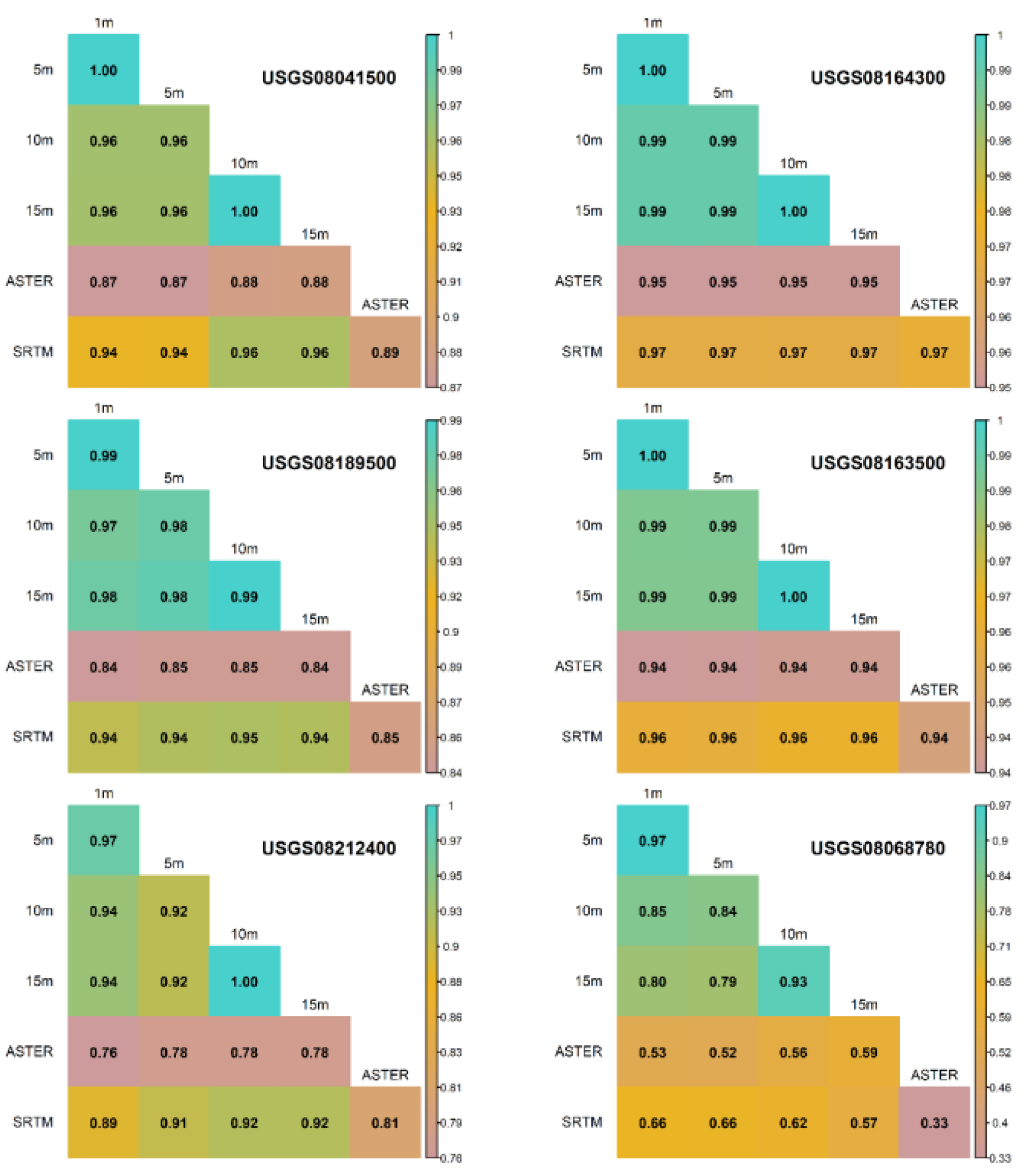
Figure 6.
Centroid distance and angle discrepancies across all watersheds and resolutions.
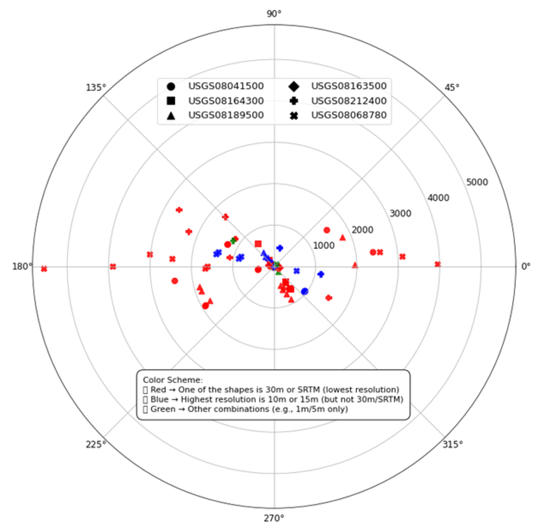
Figure 7.
Morphometric Concordance Index (MCI) metrics across watersheds and resolutions.
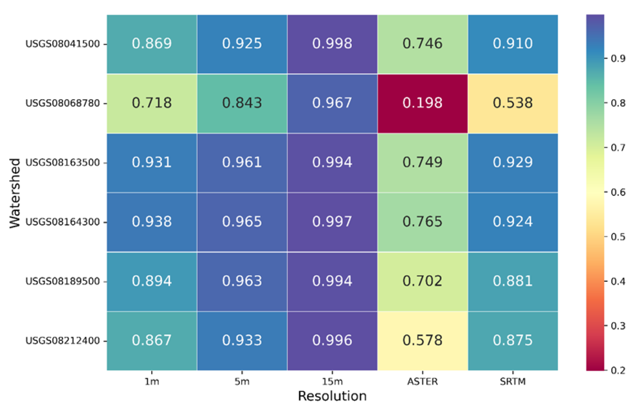
Figure 8.
TOPSIS Scores for Different DEM Products across Different Watersheds.
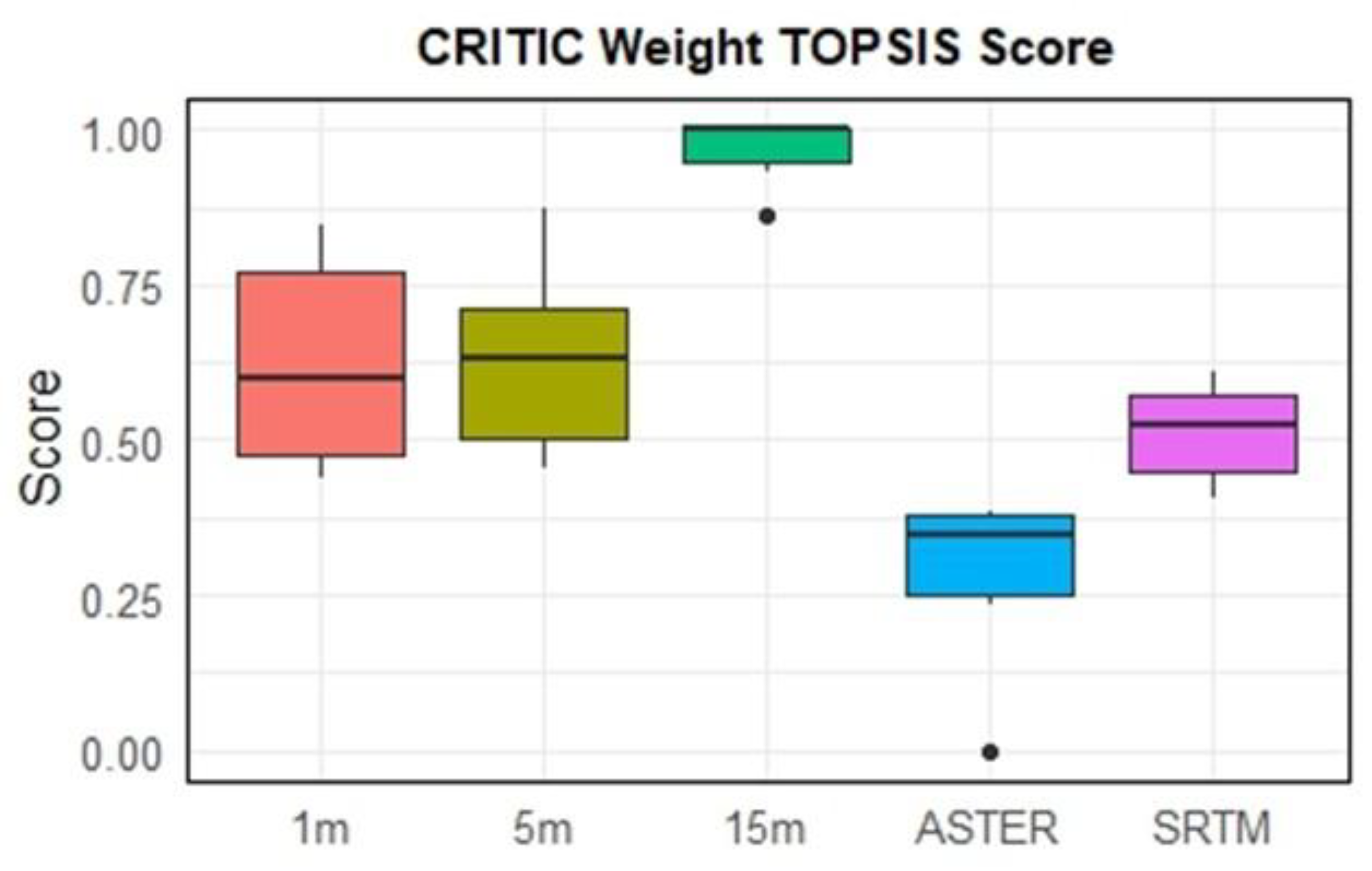
Figure 9.
Peak Flow Estimates (cfs) for a 6-Hr Unit Hydrograph across Different DEM Products at Selected Watersheds.
Figure 9.
Peak Flow Estimates (cfs) for a 6-Hr Unit Hydrograph across Different DEM Products at Selected Watersheds.
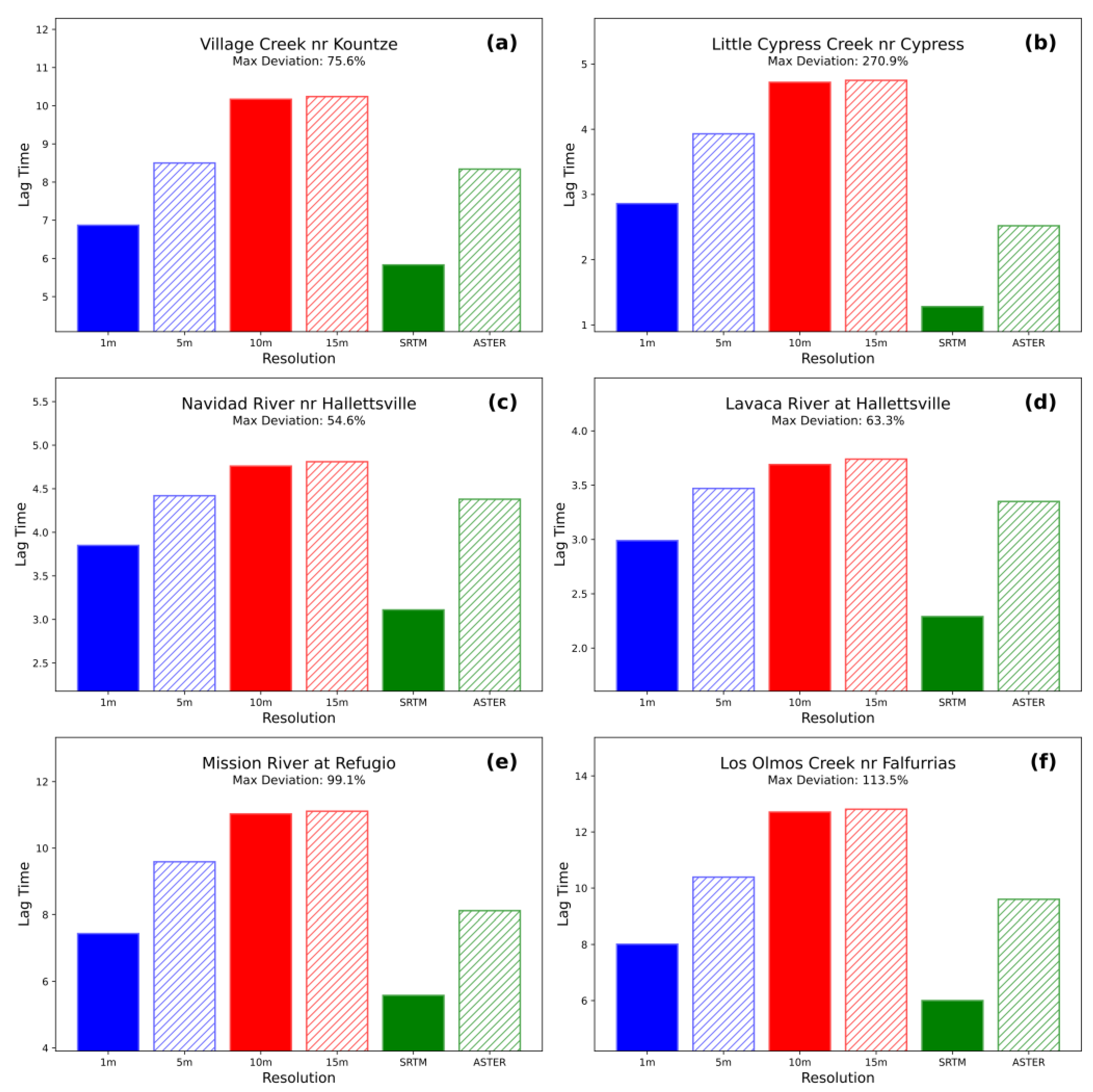
Figure 10.
Time to Peak (hr) Estimates for a 6-Hr Unit Hydrograph across Different DEM Products at Selected Watersheds.
Figure 10.
Time to Peak (hr) Estimates for a 6-Hr Unit Hydrograph across Different DEM Products at Selected Watersheds.
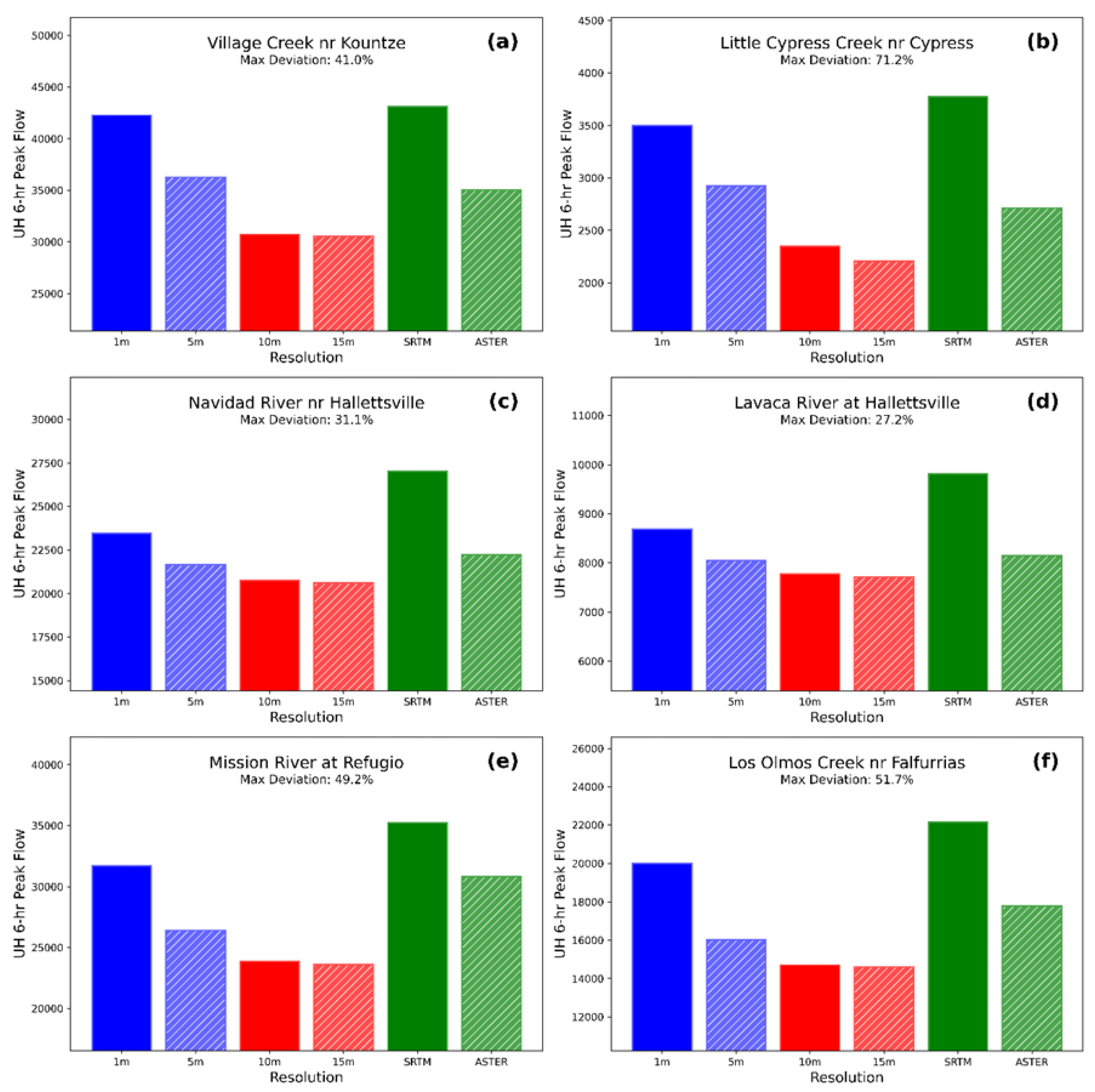
Table 2.
Terrain-Based Metrics for Evaluation.
| Parameter | Formula | Significance |
|---|---|---|
| Slope | Indicates steepness; affects runoff and erosion potential | |
| Flow Accumulation | Represents number of upslope cells contributing flow to a location | |
| Upslope Contribution Area | Estimates drainage area affecting moisture and runoff | |
| Topographic Wetness Index | Predicts potential soil moisture; higher values indicate wetter areas [41] |
Table 3.
Metrics for Evaluation of Watershed Delineations.
| Metric | Equation | Description & Utility |
|---|---|---|
| Watershed Boundary Concordance (WBC) | Measures the overall overlap between two watershed polygons. Values closer to 1 indicate high similarity. | |
| Convex Hull Containment (A ∈ B) | Quantifies how much of A’s convex hull is contained in B’s, indicating broader shape agreement. | |
| Convex Hull Containment (B ∈ A) | Same as above but in reverse; provides symmetry in evaluation. | |
| Maximum Span Distance | Identifies the maximum distance between boundary points; reflects overall spatial spread. | |
| Hausdorff Distance | Measures the largest boundary deviation; sensitive to outliers and worst-case mismatch. | |
| Centroid Distance | Represents the Euclidean distance between polygon centroids; useful for detecting positional shifts. | |
| Centroid Angle (θ) | Indicates the directional offset between watershed centroids, measured from the horizontal axis. |
Table 4.
Watershed Geomorphological Indices used for Flood Susceptibility Mapping.
| Symbol | Description | Equation | |
|---|---|---|---|
| Linear Metrics | Li | Stream Length | |
| Nu | Stream Number | ||
| I | Basin Integral Length | ||
| Br | Weighted Mean Bifurcation Ratio | Supplementary Materials S1 | |
| Aeral Metrics | A | Area | |
| Cc | Compactness Index | ||
| Dd | Drainage Density | ||
| E | Basin Elongation | ||
| Ff | Form Factor | ||
| Fs | Stream Frequency | ||
| P | Perimeter | ||
| Rc | Circularity Ratio | ||
| T | Drainage Texture | ||
| Relief Metrics | Elevation Differential | ||
| Rn | Ruggedness Number | ||
| Rr | Relief Ratio | ||
| % Slope | Basin slope |
Table 5.
Attributes of selected stations from GAGES-II dataset.
| Gauge Station ID | Station Name | Latitude | Longitude | Listed Drainage Area (sqkm) |
|---|---|---|---|---|
| USGS08041500 | Village Creek nr Kountze, TX | 30.40 | -94.26 | 2228.48 |
| USGS08068780 | Little Cypress Creek nr Cypress, TX | 30.02 | -95.70 | 114.07 |
| USGS08164300 | Navidad River nr Hallettsville, TX | 29.47 | -96.81 | 861.54 |
| USGS08163500 | Lavaca River at Hallettsville, Tx | 29.44 | -96.94 | 264.29 |
| USGS08189500 | Mission River at Refugio, TX | 28.29 | -97.28 | 1808.29 |
| USGS08212400 | Los Olmos Creek nr Falfurrias, Tx | 27.26 | -98.14 | 1236.47 |
Table 6.
This is a table. Tables should be placed in the main text near to the first time they are cited.
Table 6.
This is a table. Tables should be placed in the main text near to the first time they are cited.
| Resolution | Dataset | Source | Coverage | Collection Period |
|---|---|---|---|---|
| 1m | Neches River Basin Lidar | USGS/FEMA/Quantum Spatial and Dewberry | Neches River Basin (East Texas) | March 3-5, 2016 |
| South Central Texas Lidar | USGS/FEMA /Dewberry | Texas Counties (Atascosa, Frio, Live Oak, Gillespie, Kimble, Kerr) | Jan 4-28, 2018 | |
| Hurricane Lidar | USGS/FEMA/Furgo | 45 Texas Counties (Central to Coastal) | Jan 14 – Feb 20, 2019 | |
| South Texas Lidar | USGS/FEMA/Quantum Spatial | 30 counties in South Texas | Jan 13 – Feb 23, 2018 | |
| 1/3 Arc Sec (~10m) | 3DEP National Map Seamless | USGS | United States | June 2000 – Dec 2011 |
| 1 Arc Sec (~30m) | Shuttle Radar Topography Mission (SRTM) | NASA/NGA | Global | Feb 11–22, 2000 |
| ASTER GDEM V3 | NASA /JAXA | Global (3 arc sec) USA (1 arc sec) |
1999 – 2013 |
Table 7.
Comparison of DEM Products against 10 m (1/3 Arc-Second 3DEP Product) across Six Watersheds.
Table 7.
Comparison of DEM Products against 10 m (1/3 Arc-Second 3DEP Product) across Six Watersheds.
| Resolution | RMSE | NSE | PCC | PBIAS | R2 | ME | STD | KGE |
|---|---|---|---|---|---|---|---|---|
| 1m | 1.21 | 0.99 | >0.99 | -0.37 | >0.99 | -0.24 | 1.13 | 0.99 |
| 5m | 1.21 | 0.99 | >0.99 | -0.37 | >0.99 | -0.24 | 1.13 | 0.99 |
| 15m | 0.49 | >0.99 | >0.99 | <0.01 | >0.99 | >-0.01 | 0.49 | >0.99 |
| 30m ASTER | 6.65 | 0.79 | 0.94 | 2.10 | 0.89 | 1.23 | 5.94 | 0.88 |
| 30m SRTM | 4.67 | 0.94 | 0.98 | 4.32 | 0.97 | 3.50 | 2.95 | 0.94 |
RMSE: Root mean square error; NSE: Nash Sutcliffe Efficiency Criterion; PCC – Pearson Product Correlation Coefficient, PBIAS: Percent Bias; ME: Mean Error; STD: Standard Deviation; KGE: Kling Gupta Efficiency Metric.
Table 8.
Sinks Descriptions Observed across Six Watersheds.
| Watershed-Resolution | Sink Depth (m) | Area (m2) | Volume (m3) | |||||
|---|---|---|---|---|---|---|---|---|
| Min | Max | Mean | Median | SD | ||||
| USGS08041500 | 1m | 1.00 | 8.00 | 1.06 | 1.00 | 0.29 | 3.62E+07 | 3.83E+07 |
| 5m | 1.00 | 8.00 | 1.06 | 1.00 | 0.30 | 3.41E+07 | 3.62E+07 | |
| 10m | 1.00 | 4.00 | 1.09 | 1.00 | 0.30 | 2.90E+06 | 3.17E+06 | |
| 15m | 1.00 | 4.00 | 1.07 | 1.00 | 0.27 | 3.82E+06 | 4.09E+06 | |
| ASTER | 1.00 | 51.00 | 4.09 | 3.00 | 3.40 | 7.30E+08 | 2.99E+09 | |
| SRTM | 1.00 | 19.00 | 2.79 | 2.00 | 2.11 | 5.42E+08 | 1.51E+09 | |
| USGS08068780 | 1m | 1.00 | 11.00 | 1.59 | 1.00 | 1.37 | 5.05E+06 | 8.03E+06 |
| 5m | 1.00 | 11.00 | 1.58 | 1.00 | 1.22 | 4.50E+06 | 7.11E+06 | |
| 10m | 1.00 | 4.00 | 1.28 | 1.00 | 0.58 | 1.80E+06 | 2.30E+06 | |
| 15m | 1.00 | 4.00 | 1.28 | 1.00 | 0.58 | 1.85E+06 | 2.37E+06 | |
| ASTER | 1.00 | 20.00 | 2.99 | 2.00 | 2.16 | 3.06E+07 | 9.14E+07 | |
| SRTM | 1.00 | 11.00 | 1.74 | 1.00 | 1.03 | 2.32E+07 | 4.04E+07 | |
| USGS08164300 | 1m | 1.00 | 8.00 | 1.20 | 1.00 | 0.55 | 1.03E+07 | 1.24E+07 |
| 5m | 1.00 | 8.00 | 1.19 | 1.00 | 0.55 | 9.95E+06 | 1.19E+07 | |
| 10m | 1.00 | 138.00 | 3.21 | 1.00 | 14.23 | 2.15E+06 | 6.90E+06 | |
| 15m | 1.00 | 138.00 | 2.72 | 1.00 | 12.45 | 2.98E+06 | 8.12E+06 | |
| ASTER | 1.00 | 33.00 | 3.81 | 3.00 | 2.99 | 2.81E+08 | 1.07E+09 | |
| SRTM | 1.00 | 13.00 | 2.16 | 2.00 | 1.59 | 1.44E+08 | 3.11E+08 | |
| USGS08163500 | 1m | 1.00 | 5.00 | 1.13 | 1.00 | 0.40 | 3.25E+06 | 3.68E+06 |
| 5m | 1.00 | 5.00 | 1.14 | 1.00 | 0.41 | 2.98E+06 | 3.39E+06 | |
| 10m | 1.00 | 121.00 | 4.69 | 1.00 | 17.84 | 5.93E+05 | 2.78E+06 | |
| 15m | 1.00 | 121.00 | 3.49 | 1.00 | 14.73 | 9.22E+05 | 3.22E+06 | |
| ASTER | 1.00 | 25.00 | 3.58 | 3.00 | 2.71 | 8.21E+07 | 2.94E+08 | |
| SRTM | 1.00 | 10.00 | 1.57 | 1.00 | 0.91 | 3.40E+07 | 5.36E+07 | |
| USGS08189500 | 1m | 1.00 | 13.00 | 1.24 | 1.00 | 0.77 | 1.80E+07 | 2.23E+07 |
| 5m | 1.00 | 13.00 | 1.22 | 1.00 | 0.76 | 1.76E+07 | 2.15E+07 | |
| 10m | 0.10 | 5.80 | 0.52 | 0.30 | 0.60 | 1.06E+07 | 5.53E+06 | |
| 15m | 0.10 | 5.80 | 0.56 | 0.30 | 0.61 | 1.40E+07 | 7.76E+06 | |
| ASTER | 1.00 | 40.00 | 3.06 | 2.00 | 2.39 | 4.80E+08 | 1.47E+09 | |
| SRTM | 1.00 | 20.00 | 1.61 | 1.00 | 0.94 | 3.31E+08 | 5.33E+08 | |
| USGS08212400 | 1m | 1.00 | 9.00 | 1.46 | 1.00 | 0.84 | 2.35E+07 | 3.43E+07 |
| 5m | 1.00 | 9.00 | 1.46 | 1.00 | 0.87 | 2.14E+07 | 3.12E+07 | |
| 10m | 0.10 | 6.30 | 0.83 | 0.50 | 0.87 | 1.82E+07 | 1.50E+07 | |
| 15m | 0.10 | 6.40 | 0.81 | 0.50 | 0.86 | 2.00E+07 | 1.63E+07 | |
| ASTER | 1.00 | 51.00 | 4.23 | 3.00 | 3.87 | 3.35E+08 | 1.42E+09 | |
| SRTM | 1.00 | 17.00 | 1.56 | 1.00 | 0.92 | 1.81E+08 | 2.83E+08 | |
Disclaimer/Publisher’s Note: The statements, opinions and data contained in all publications are solely those of the individual author(s) and contributor(s) and not of MDPI and/or the editor(s). MDPI and/or the editor(s) disclaim responsibility for any injury to people or property resulting from any ideas, methods, instructions or products referred to in the content. |
© 2025 by the authors. Licensee MDPI, Basel, Switzerland. This article is an open access article distributed under the terms and conditions of the Creative Commons Attribution (CC BY) license (http://creativecommons.org/licenses/by/4.0/).
Copyright: This open access article is published under a Creative Commons CC BY 4.0 license, which permit the free download, distribution, and reuse, provided that the author and preprint are cited in any reuse.


