
Submitted:
26 August 2025
Posted:
27 August 2025
You are already at the latest version
Abstract
A reliable Digital Elevation Model (DEM) is a key input for land use planning and risk management, particularly in floodplains where low-resolution models often fail to represent subtle topographic variations. In many regions worldwide, high-precision elevation data are unavailable, necessitating the development of methods to enhance existing global digital elevation models (DEM). This study proposes a practical and replicable methodology to improve the vertical accuracy of global DEMs in flat terrains with limited data availability. The approach is based on correcting the altimetric differences between the DEM and GNSS-RTK-surveyed topographic points, incorporating land cover classification to refine adjustments. The methodology was tested in the Ranchería River delta in Riohacha, La Guajira, Colombia, using four global DEMs: FABDEM, SRTM, ASTER, and ALOS. Results showed a significant reduction in root mean square error (RMSE), with improvements of up to 76.691% for ASTER, 55.882 % for FABDEM, 55.932 % for SRTM, and 36.842 % for ALOS. The proposed method requires minimal computational resources and no advanced programming. Due to minimal data requirements, it makes it a scalable and replicable solution for similar floodplain environments. These enhancements in local altimetric accuracy could help to improve the reliability of hydrodynamic modeling, with direct implications for flood risk management and decision-making in vulnerable flatland areas.
Keywords:
DEM-correction
; GNSS-RTK
; floodplains
; FABDEM
; SRTM
; ASTER
; ALOS
1. Introduction
Floodplains are defined as the flat area (slope less than 3 %) surrounding the active channel of a river, which are flooded during high discharge events, every one or two years [1]. Within these floodplains are deltas and valleys [2,3]. These are areas conducive to economic development, agriculture, and community settlement [4]. In recent decades, growth in population in floodplains [5], together with more extreme and intense rainfall events caused by phenomena such as EL NIÑO/LA NIÑA [6], has increased the risk of flooding in many of these places around the world [5]. Faced with this scenario, it is necessary to implement risk reduction strategies, which require good quality geo-spatial inputs and the use of modeling tools that generate useful information for decision-making [6].
One of the most important inputs for land use planning and risk management applications is the altimetrically reliable Digital Elevation Model (DEM) [7], particularly challenging in flat terrain where low-precision global models cannot represent the terrain configuration in enough detail [8]. Applications like flood zone mapping, river delineation, and definition of restoration zones rely heavily on accurate DEMs due to their direct impact on model reliability [9,10].
Currently, DEMs are mainly created by remote sensing techniques, due to the ability to map large areas with low personnel requirements and at lower cost [11]. Among the remote sensing techniques are photogrammetry, Interferometric Synthetic Aperture Radar (In-SAR), and Light Detection and Ranging (LIDAR) [7]. These types of elevation models have vertical errors, with LIDAR having the lowest vertical errors (generally <1 m) [7] while models such as FABDEM derived from COPERNICUS DEM, that is based on InSAR sensor [12,13,14], SRTM based on radar [15], ASTER based on optical stereo image pairs [16], and ALOS also based on radar techniques as SRTM but with a different processing [17], have errors ranging from 1.12 m to 10 m [12,18,19,20].
Additionally, these models contain attributes from different objects present in the terrain, both natural (vegetation) and man-made (buildings, communication towers, among others), that need to be removed to have the bare terrain. This is why multiple filtering and classification techniques have been developed and applied to extract terrain points to generate the corrected DEM [21,22,23]. Despite these efforts, none of these techniques is 100% effective in removing all objects that do not belong to the terrain, which makes further editing necessary to generate a DEM suitable for the application of modeling tools [24]. Additionally, global models do not have sufficient spatial resolution to be able to represent small terrain structures, such as connecting channels between the main river and floodplains, roads, and levees [25], which are necessary for flood mapping [26].
Different techniques have been developed and applied to perform corrections to global DEMs and improve their accuracy; among the most commonly used techniques for DEM correction are: data fusion (hybridization) [27], masking of water bodies [28], gap filling [29], channel burning [30] and vegetation removal [8,31]. More recently, the application of machine learning techniques to perform DEM enhancement has been explored [7,12,32,33]. The methodologies presented above have proven effective in improving the vertical accuracy of global DEMs. However, there are certain limitations of these methodologies to achieve the levels of DEM accuracy and detail required for different land use planning and risk management applications. Among these limitations, a common one is the scale of application of these methodologies; most have been applied at a regional or quasi-global scale, and the field information included in the methodological flow is insufficient, which does not allow for an optimal level of detail at the local scale of the resulting product. Considering that land-use planning and risk management exercises are conducted at local scales, this is a crucial aspect.
Based on the above, this article proposes a methodology that combines global remote sensing with locally surveyed field information to improve the vertical accuracy of digital elevation models in flat areas with limited information. The Rancheria River Delta (La Guajira, Colombia) will be used as a case of application of the proposed methodology.
2. Materials and Methods
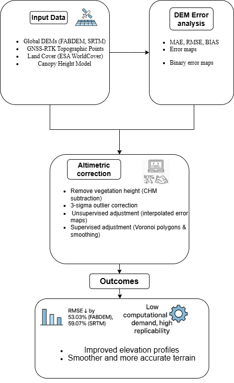
The correction method proposes the use of information derived from remote sensors (land cover, tree height) combined with information acquired in the field (topographic points) to perform the altimetry correction of global digital elevation models. This methodology is proposed in a sequential flow, starting with a preliminary stage in which the study area is selected and all necessary information is collected and prepared for DEM correction. Next, an error assessment of the DEMs is conducted, followed by the correction. A summary of the stages of the method is presented in Figure 1, and each of these stages will be developed in the following sections.
2.1. Preliminaries
2.1.1. Criteria for Study Area Selection
The study area should be one of the plain areas, such as alluvial plains, valleys, and deltas, which suffer from periodic flooding due to the overflow of an active river channel, defined by [1,2], where terrain variations are less than one meter in several thousand meters of extension, slopes less than 3% [34]. These areas must have the presence of an active river that causes periodic flooding.
2.1.2. Gathering and Preparation of Input Data
The following are the minimum information requirements for the application of the proposed methodology:
- Digital Elevation Models (DEM) at least medium resolution (between 10 and 30 m) are required, such as global models (SRTM, ASTER, ALOS, FABDEM- COPERNICUS);
- Land Cover information is necessary to identify the presence of structures such as houses, buildings, roads, vegetation zones, and water bodies in the study area;
- Tree height information CHM (Canopy Height Model) to perform altimetric correction of global models, since these models, being surface models, take into account the heights of elements on the ground, such as vegetation and buildings. Several global CHM products can be used to correct tree elevations in global DEMs [35,36,37]
- Thematic vector information, such as roads, streets, buildings, and rivers, is very important to identify key terrain elements. This information is available through https://www.openstreetmap.org/#map=14/11.5361/-72.8656, OpenStreetMap;
- Topographic information. High-precision elevation data should be collected using precision equipment such as GNSS-RTK or Total Station, with which an accuracy (<10 cm). Providing ground control points distributed across the study area. These data are essential for assessing the vertical accuracy of DEMs and for the correction process.
2.2. DEM Error Analysis
2.2.1. Error Calculation
A vertical accuracy assessment of DEMs must be performed to determine their fit with respect to the topography points surveyed. First, elevation of DEM is extracted at each point, then the error is calculated whit Equation (1).
Points must be divided into a data set for error assessment and make the adjustment, and another set for validation of the performance of the applied correction method [7,32]. There is no unique relation to divide the evaluation and validation data of the elevation models; different distributions of the quantities must be tested, depending on the amount of data available, evaluating the results obtained to determine the most optimal in each case.
2.2.2. Error Metrics
Error metrics are used to evaluate the performance or fit of the models concerning the observed data. The following metrics are commonly used: MAE (Mean Absolute Error) [12,38] (Equation (2)), RMSE (Root Mean Square Error) [7,31,32,33] (Equation (3)), BIAS (Equation (4)), which measures the average tendency of the model data to overestimate or underestimate the true value (field data) [32], and STD (Standard Deviation) (Equation (5)) [39].
where: : Elevation of the surveyed point; : Elevation of the point extracted from the DEM; n: Number of points evaluated; : Mean Error.
2.2.3. Error Map
Metrics can give an averaged measure of the model’s fit to the field data; however, metrics cannot determine the spatial distribution of these errors, which is important when applying DEM correction procedures. To appreciate the spatial distribution of the errors, error maps must be generated. They are made by interpolating differences to create a data grid in raster format (GeoTiff). Several spatial interpolation methods must be tested to generate the error maps, such as IDW, Kriging, Natural Neighbor, Nearest Neighbor, among others, which are available in different GIS tools [40,41].
2.2.4. Binary Error Map
As differences can be negative and positive, it is necessary to identify in which areas the DEM is above and in which areas it is below the points. To have clarity about this behavior, the error maps should be classified to generate a binary map of 0 and 1, in which 0 indicates negative differences, i.e., the DEM pixel value is greater than the terrain points, and 1 indicates positive differences, where the terrain point value is greater than the DEM pixel value.
2.3. DEM Vertical Correction Method
Once the models have been evaluated, they are corrected. The DEM altimetry correction process is divided into four steps, which are presented below.
- i
- Vegetation heights removal. This step consists of subtracting from the DEM the vegetation heights of the CHM. This operation is performed using a raster calculator tool, which subtracts the CHM from the DEM. In this step, a DEM with removed vegetation heights is obtained.
- ii
- Outliers Correction. The 3-sigma criterion is applied to eliminate outliers in the distribution of elevations from the DEMs. This criterion states that all values of a data distribution must be located between the limits: average - 3 standard deviations to average + 3 standard deviations, and any value located outside these limits is considered an outlier [42]. This has been applied in multiple DEM correction cases [43,44,45]. This method is applied using an algorithm that goes through the DEM pixel by pixel, comparing the value with the 3-sigma calculated for that DEM. If it finds a pixel with a higher value, that value is replaced by the 3-sigma value.
- iii
- Unsupervised adjustment. This step should refine the DEM by incorporating surveyed terrain points through error maps derived from interpolation methods. It is considered “unsupervised” because the outcome depends on interpolation parameters, with limited control over the final surface; nevertheless, it provides a reliable approximation. The procedure begins by evaluating the binary error map: for pixels coded as 0, the DEM should be corrected by subtracting the absolute error value, while for pixels coded as 1, the error value should be added. Two raster grids are generated, each containing the adjusted values for their corresponding pixels. These grids are then merged to produce the final corrected DEM. This process can be seen schematically in Figure 2;
- iv
- Supervised adjustment. This step is required to address residual errors propagated from the interpolation used in error map generation. The procedure should begin with the creation of Voronoi polygons [46,47] from terrain control points. These polygons must then be grouped into homogeneous elevation zones, each assigned with a threshold value that defines its elevation limit. After rasterization of the polygons, the resulting raster should serve as a mask for DEM correction. Using a 3×3 moving window, DEM pixels are iteratively evaluated against the elevation limits defined by the mask. Pixels exceeding the threshold should be replaced with the mean of their eight neighboring values, and the process repeated until no violations remain.
3. Results
3.1. Preliminaries
3.1.1. Study Area
The chosen study area corresponds to the Rancheria River Delta, in the city of Riohacha, La Guajira, Colombia. The Rancheria River Delta is located northeast of the town. Figure 3 shows the general location, the layout of the main channel of the Rancheria river (1) that bifurcates close to the coastline, giving rise to two branches that form the delta, El Riito (2) and Santa Rita (3), the latter bifurcating again to give rise to the Calancala branch (4) [48].
3.1.2. Information Gathered and Processed
Information used for the methodology is presented below.
-
Digital Elevation Models (DEM’s). FABDEM (Forest And Buildings removed DEM). It is a global digital terrain model derived from Copernicus DEM. It has a spatial resolution of 30 m and covers latitudes between ±60°. Its development was based on machine learning techniques trained with LiDAR data and land cover layers, which significantly improves accuracy in forested and urban areas compared to other similar models [12].SRTM (Shuttle Radar Topography Mission). It was conducted over 11 days in February 2000, collecting C-band synthetic aperture radar (SAR) data over terrestrial areas between 60°N and 56°S, representing about of the total land mass [18]. Version 3 of the SRTM DEM with 30 meters spatial resolution, published in 2015 [49], was used.ASTER GDEM. Terra’s Advanced Thermal Emission and Reflection (ASTER) Spatial Radiometer Global Elevation Digital Model (GDEM) Version 3 (ASTGTM) provides a global digital elevation model (DEM) of Earth’s terrestrial areas with a spatial resolution of 30 m [28,50].ALOS (ALOS WORLD 3D DEM). Between 2006 and 2011, the Panchromatic Remote Sensing Instrument for Stereoscopic Mapping (PRISM) sensor aboard the ALOS (Japan Aerospace Exploration Agency) satellite captured stereoscopic images with a resolution of 2.5 m [20,51]. These images were used to produce a commercial DEM of very high resolution (0.15 arcseconds) ALOS World 3D (AW3D), which was subsequently resampled to obtain the open-access DEM ALOS World 3D 30 m (AW3D30), with a resolution of 30 m [20,51]. Version 3.2 was used, the latest available [52]. Figure 4 shows the cropping of the used DEMs to the study area;
- The European Space Agency (ESA) https://viewer.esa-worldcover.org/worldcover/?language=en&bbox=-1.648666525072074,53.78498239999999,-1.4636494749279256,53.8349824&overlay=false&bgLayer=OSM&date=2024-01-23&layer=WORLDCOVER_2021_MAP, ESA WorldCover 2021 v200 [53] was used as a basis to generate a classified map of the study area. The land cover map can be seen in Figure 5;
- The Global Forest Canopy Height Model, 2019 from https://glad.umd.edu/dataset/gedi/, GLAD- Global Land Analysis and Discovery [36] was used. Figure 6 shows the cropping of the study area;
-
The field topographic information was surveyed in two campaigns carried out in the study area, one in September 2022 and the other in March 2023. The topographic points were surveyed with GNSS-RTK in dynamic mode, with TOPCON Hyper V equipment, which has a horizontal accuracy of 0.005 m and vertical accuracy of 0.01 m [54]. The database used for the base station location is the one that includes points from Colombia’s national active and passive leveling network, managed by the Instituto Geográfico Agustín Codazzi (IGAC). These points can be viewed through the data portal https://www.colombiaenmapas.gov.co/?e=-74.16992317492544,4.422176247962095,-74.02795921618541,4.531019801595585,4686&b=igac&u=0&t=25&servicio=472, Colombia en Mapas. The points near the study area were located, and the point belonging to the MAGNA ECO ACTIVE NETWORK (11°30’47.58123"N -72°52’10.95231"W) located at University of La Guajira, this point was chosen because it is located on the roof of a building, which offers an advantage in terms of the signal range of the base equipment and its link with the ROVER, also at this point there were security conditions to leave the equipment without the need for a person in charge of its security, while the survey of the points was being carried out.The location of the points was determined during the survey planning, taking into account the land cover in the area, to place points in all identified zones. A series of points was located on the classified map, covering all land cover categories, and these were equidistant from each other. However, during the survey’s execution, it was not always possible to adhere to the planned approach. Consequently, a quasi-random field-survey method was employed due to accessibility limitations caused by flooded areas, public order situations within the territory, and unfavorable vegetation conditions, which hindered the reception of the GNSS-RTK equipment. The survey was conducted by traveling through the study area, depending on accessibility conditions; in some areas, it was done by vehicle (motorcycle), and in others, by walking. Points were surveyed in areas of interest (i.e., plains, near areas of thick vegetation, embankments, roads, housing areas, and elevated areas), trying to capture with the best possible detail the terrain configuration. The ROVER equipment was constantly checked to ensure that it was operating under optimal conditions of satellite reception and connection with the base station.Figure 7 shows the points surveyed in the study area, which totaled 1016, including terrain points, elevation points of terrain structures, and river points.
3.2. DEM Error Spatial Analysis
Different distributions of points for adjustment and validation were tested. Better results in error metrics reduction were found with the distribution () for adjustment and validation, respectively. From surveyed points, only the terrain points were selected for the analysis of DEMs. 707 terrain points were used, which were divided into 75% (530) for the adjustment and 25% (177) for validation. The elevation of the DEMs was extracted for each of the points, and the error concerning their elevation was determined. The errors in the FABDEM are in the range between to m for the SRTM, between to m, for ASTER between to m and for ALOS, between to . The magnitude of the errors between DEMs is very similar, except for ASTER. Figure 8 shows the distribution of errors and metrics by DEM. The tendency of errors, except for the SRTM, is to overestimate the value of the true elevation, as can be seen in the density curves of errors in Figure 8, and for the sign of BIAS. FABDEM generally performs better in all metrics, except for BIAS, where SRTM and ALOS outperform, and ASTER performs poorly across all metrics. The metrics results are within the expected range for these models [12,55].
The metrics, being measurements of specific points, do not allow observing the spatial distribution of the errors. For this purpose, error maps and binary maps of these errors were generated, which can be seen in Figure 9 and Figure 10.
Error maps and binary maps confirm the tendency shown by density curves and BIAS in Figure 8. For FABDEM, ASTER, and ALOS, error maps have mostly negative values, and the binary maps are mostly 0, while for SRTM, the error map is mostly positive and the binary map is mostly 1.
3.3. Output of Proposed Method
The procedure described in Section 2.3 of the methodology was applied to obtain the altimetrically adjusted DEM. The result of the correction was evaluated by the error metrics described in Section 2.2. Figure 11 presents the error distribution and error metrics taken from the DEMs after applying the correction process, compared with the same before the correction, and Table 1 presents a summary of metrics before and after the correction process, with the percent reduction for each metric.
As can be seen in Figure 11, the correction method results in a significant reduction in error metrics. The reduction is different for each metric across the DEMs. Figure 11 also demonstrates the change in error distribution in density curves. It can be seen how the correction method fits the errors to zero; most of the density of residual errors is closer to zero. This behavior is better observed by box plot graphs. Figure 12 shows the box plot for all DEMs, original and corrected. Box plots show how the correction method adjusts the distribution of the residuals in the two DEMs and brings the median closer to zero. Initially, the outliers are considerably separated from the extremes of the graph. When the adjustment is applied, the variability of the residuals decreases, and it can be observed how the extremes become thinner and closer to the center, and the outliers also become closer to the extremes of the graph.
According to the results in Table 1, the correction method achieves a significant reduction of the error in DEMs, as can be seen in the different metrics. For the RMSE, which is one of the most used metrics, a reduction of the error is % for FABDEM, % for SRTM, % for ASTER, and % for ALOS. ASTER has the highest percent reduction in metrics, with % for MAE and % for STD, while ALOS has the lower percent reduction with % and % for MAE and STD, respectively. FABDEM and SRTM are in the middle, with % and % the FABDEM and % and % for SRTM, for MAE and STD, respectively. The BIAS also shows a significant reduction, going from to in FABDEM, also showing a change in the trend, same situation for ASTER ( to ) and ALOS ( to ) the BIAS not only changed magnitude, while in SRTM it went from to keeping its trend. Figure 13 shows the DEMs corrected altimetrically.
Another way to appreciate the change in DEMs with the application of the correction is by using terrain profiles to see the difference in elevations between the original DEM and the corrected DEM. Figure 14 shows the used profiles. Figure 15 shows the profiles obtained for each DEM before and after applying the correction process. Likewise, profiles were made to compare all DEMs before and after the application of the correction process. These comparison profiles between DEMs are shown in Figure 16.
Figure 15 shows the effect of applying the correction method. Before applying the correction, DEMs exhibit significant variability and exhibit extreme elevation changes. Profiles also show a tendency for elevations in DEMs for FABDEM, ASTER, and ALOS original profiles to be above the corrected ones, which coincides with the BIAS, while the SRTM original profile is below the corrected one. After applying the correction, profiles show a significant change in elevation and present a smoother distribution of elevation along the longitudinal profiles. Longitudinal profiles demonstrate that the method is effective in generating a softened surface in the DEM and eliminating random peaks and outliers in elevation. The range of elevation profiles changes from to in the original DEMs, to to in corrected DEMs. The variability in profiles represented by the mean standard deviation between the four profiles was also reduced; in FABDEM, it was reduced from to , in SRTM from to , in ASTER from to , and for ALOS from to .
As can be seen in Figure 16, before the application of the correction method, DEMs present a great difference between them. This coincides with the results of the evaluation of the error of the DEMs before the application of the correction method, which shows the difference in the trend of the errors between DEMs and the field data.
FABDEM, ASTER, and ALOS tend to overestimate the real elevation data, while the SRTM tends to underestimate the real elevation. This is evident in the profiles, where it is observed that FABDEM, ASTER, and ALOS generally exceed the SRTM, except at specific points where the SRTM features elevation peaks. With the application of the correction, it is possible to reduce the differences between the DEMs.
This has already been observed with the result of the BIAS presented, which shows a decrease in its dimension for all DEMs, the tendency of the errors is inverted for FABDEM, ASTER, and ALOS. Also, the profiles in Figure 16 show how, after the application of the correction, the difference between the DEMs is reduced; however, it can be observed that they still have some extreme peaks at some points, but the difference between them is reduced.
4. Discussion
The results presented suggest that the proposed methodology can correct a large percentage of the errors given by the digital elevation models. However, although the methodology is shown to be simple, it is convenient to discuss a series of aspects that are involved around it and the results. The discussion is given in two instances: firstly, on the aspects to consider in the preparation and analysis of the input information, and secondly, on the results shown in the correction of the DEM.
4.1. Input Data Used and Processing
The methodology presented here has an advantage over other, more complex methods in terms of the amount and variety of information needed for its application. In this methodology, the main input of information is the topographic points, and it is essential to be clear about the quantity and density of these in the study area. Regarding these, there are no references in the literature that can indicate precise and applicable values for all cases; this being a determination of each investigation, according to the needs and objectives that are had.
In this study, the number of points and their location were initially defined in the planning of the field campaigns according to the identified land covers, seeking to have points in the different zones; later, at the time of conducting the campaigns, other factors specific to the field were taken into account, such as accessibility, security conditions, and environmental conditions that influenced the execution of the field campaigns. The number of points finally obtained was based on the weighting of all these conditions and the criteria of the research team, taking into account the characteristics of the study area; an optimum number was considered for the DEM adjustment process. Another important topic to discuss about points is the survey method. As the approach adopted was quasi-random, it is possible that in future work with the availability of points in all the land cover classes, the accuracy can change; for example, with points in dense vegetation zones, the accuracy can decrease. Other survey methods, such as a Total station, or data from the GEDI-LIDAR sensor [56], should be considered if available in the study area. To apply the methodology to other study zones with similar characteristics, and based on the results of error reduction, a minimum density of 25 points per square kilometer of study area was determined. In addition to considering that, the points should be located in the different classes of land cover identified. However, it should be noted that this value is not an absolute standard; the density of points that can be obtained depends on all the factors mentioned above, which vary in each case.
On the other hand, the number of points used for the adjustment process and validation is also a value that can vary from one case to another, and there is no exact value that applies to all [7,32]. Different combinations of the distribution of points were tested to evaluate the results in decreasing the error in the DEMs, finding that the used distribution yielded the best results. Obtaining a higher reduction percentage is with the 75 % for the adjustment and 25 % for the validation, which was the distribution used, as presented in Section 3.2. These percentages of division of the points allow avoiding overfitting and having an optimal number of points for validation [12]. Another important topic to discuss is the partitioning method; in this paper, a random sampling was employed. Considering the method for the survey, this was the most suitable approach. However, the use of advanced partitioning strategies is not completely discouraged and could be for future work to improve the results of the method.
4.2. Error Assessment and DEM Correction
The error metrics used in this study agree with those widely used in the scientific community to evaluate the performance of altimetry correction methodologies of DEMs, the most widely used being the RMSE [12,33,57]. However, these metrics are not suitable for data that do not follow a normal distribution [39]; for the analyzed DEMs, this limitation discards, with the density curves present in Figure 7, that demonstrate that errors in DEMs follow a normal distribution, validating metrics selection. Both RMSE and MAE are scale-dependent metrics, i.e., they show the error in the same unit as the studied variable. The main advantage of these metrics is their easy calculation and interpretation [58,59,60]. However, since these metrics are averaged, they are limited in identifying trends in the errors. Therefore, it was necessary to use the BIAS, a metric that indicates the model’s tendency to overestimate or underestimate real values. It can take negative or positive values, with values closer to zero indicating less deviation or error of the model concerning the real data [32,61]. This, makes necessary the use error and binary error maps, for the spatial error analysis as were used in this research.
The removal of tree heights using the Canopy Height Model (CHM), and the removal of outliers by the 3-sigma criterion, constitute a good first approximation to the DEM correction; however, altimetry errors that do not come from the vegetation will prevail in the DEM, which makes necessary the application of the subsequent process proposed in this article.
The results show that a significant reduction in the error of DEMs is achieved; for RMSE, a reduction between % and % is achieved, while for MAE the reduction is between % and %. These results demonstrate the effectiveness of the method, given the minimal information required and its low complexity, compared to other methodologies that necessitate significantly more information and, consequently, higher computational and processing capacities. Such methodologies that apply machine learning algorithms [7,12,32,33], with which reductions of up to 80% of the RMSE are achieved. However, these methodologies require large amounts of information, in addition to extensive knowledge in programming these algorithms, which may limit their application. The methodology proposed in this article is offered as a less complex alternative to be applied, which offers a greater potential to be replicated in similar areas. However, is important to keep in mind the possible errors due to the methods used, mainly the interpolations made to generate the error maps, which were used as a DEM correction surface. It was made to minimize these errors using different interpolation methods to obtain an averaged surface between them. This strategy allowed reducing the appearance of artifacts coming from the interpolation in the surfaces; however, it is kept in mind that they cannot be completely avoided, and the remaining errors presented in the final DEMs are influenced by these errors inherent to the interpolation methods.
About the correction process, presented in Section 2.3, some clarities are necessary. The process is presented in four stages to provide a coherent workflow; however, it is important to declare that each stage has a different effect on the final results. First and second stages act more as data curation than correction properly, because both do not reduce significantly the error metrics. For example, the RMSE after applying vegetation and outlier removal is still equal for FABDEM and ALOS; this had few changes for SRTM that decreased from to () and for ASTER that decreased from to (). This two stages had effect on the elevation ranges of DEMs. FABDEM changed its range ( to ) to ( to ), SRTM from ( to ) to ( to ), ASTER from ( to ) to ( to ), and ALOS from ( to ) to ( to ). The obtained reduction percent in metrics is reached in unsupervised and supervised adjustment stages. The RMSE for FABDEM went from to , a reduction of in unsupervised adjustment, for SRTM to , a reduction of , for ASTER to , a reduction of , and for ALOS to , a reduction of .
FABDEM presented better performance in metrics, even in the initial evaluation, as in the corrected DEM. This result follows the expected, because FABDEM is an improved version of another global DEM, the COPERNICUS [12,62]. On the other hand, errors in SRTM, ASTER and ALOS are within the expected range for this kind of DEMs [55]. Additionally, the fact that it is a reprocessed DEM also distinguishes the FABDEM from the others in terms of age. ASTER, SRTM, and ALOS are older missions than COPERNICUS, from which the FABDEM is derived [39]. This factor also influences the accuracy of the DEMs, due to changes that occur on the ground in terms of coverage and interventions, which can significantly modify the terrain in areas of urban growth. Tendency of errors for each DEM is an important topic to discuss. Generally global DEMs tend to overestimate the ground surface elevation, especially in flat areas [63,64]. This behavior was presented for FABDEM, ASTER, and ALOS; however, SRTM has presented an opposite tendency. This is because SRTM in low-lying and coastal areas tends to underestimate [65,66,67].
The remain errors in DEMs have implications for their potential applications. For example, the remain RMSE of for FABDEM, SRTM, ASTER, and ALOS. Should affect their application for flood modeling in flood plains, where DEMs with RMSE below 1 m are ideal [26,68]. According to results, the final RMSE obtained for FABDEM meets the minimum requirement for flood modeling in flood plains. However, the accuracy level achieved is not equal to using a high precision DEM such as LIDAR or UAV-derived DEMs [69,70]; nevertheless, for data scarce areas, FABDEM, after applying our correction method, would be a suitable option.
5. Conclusions
This study presents the development of a methodology for global DEM correction in floodplain areas. The methodology uses freely available open source DEMs of medium resolution (30 m), remote sensing information such as land cover, tree height model, and local field topographic information surveyed with GNSS-RTK. The correction methodology allows obtaining a significant improvement between % and % of the RMSE concerning the initial error between the DEM and the field points.
Specifically, an RMSE of m is achieved in the FABDEM, which is a significant improvement for this type of DEM of global coverage, considering the initial RMSE of m. SRTM, ASTER, and ALOS achieved an RMSE of , , and , respectively. Despite the significant vertical error reduction in SRTM, ASTER, and ALOS DEMs, FABDEM is recommended for use in areas where high-precision DEMs such as LIDAR are unavailable, and by applying improvement techniques, it can be used for various applications, especially territorial planning and risk management.
Error and binary maps generated in this study demonstrate that they are handy tools for spatially analyzing the error in digital elevation models. In contrast to statistical metrics, which only summarize errors as average values, these maps allow for the observation of the spatial distribution of errors and their tendency around the study area.
For instance, the developed methodology is presented as an easy-to-apply alternative with low information and processing requirements compared to other local methodologies, offering an advantage for DEM altimetry correction and being optimal for the required local applications. This situation is common in areas with a lack of information. The results show the key factor in the improvement obtained in the elimination of vegetation and the reduction in building heights.
The product generated using the developed methodology must later be subjected to a hydrological-hydraulic conditioning process to make it optimal for these applications. As a future work of the methodology presented in this article, it is proposed to apply a hydraulic conditioning process to the DEM, to make it optimal for applications that require, in addition to vertical accuracy, a good bathymetric representation, such as those that apply hydrodynamic modeling.
Summarize, the aforementioned methodology can significantly enhance global models in situations where we must employ global DTMs (DEMs). However, more precise models such as those derived from LiDAR scanning, are required for precise flood modeling and analysis. The proposed method offers a technically and operationally feasible solution for improving DEM accuracy in data-scarce floodplains, supporting local authorities, environmental agencies, and researchers involved in local-scale flood risk assessment and land use planning.
Funding
This work was carried out as part of the PhD project of Jose Fragozo and was financially supported by the Ministerio de Ciencia, Tecnología e Innovación (Minciencias), Colombia. The Universidad de La Guajira covered the Article Processing Charge (APC)
Acknowledgments
The authors wish to express their sincere gratitude to the Ministerio de Ciencia, Tecnología e Innovación, de Colombia (Minciencias), under Call 890-2020, Project No. 82207, with financial resources administered by the Instituto Colombiano de Crédito Educativo y Estudios Técnicos en el Exterior (ICETEX), for enabling the contribution of Dr. Jairo René Escobar Villanueva in providing valuable advice throughout this study. The authors also extend their thanks to the Pontificia Universidad Javeriana for their logistical support during the topographic field campaigns, particularly for providing access to GNSS RTK equipment. We thank the Universidad de La Guajira for their support in the logistical planning of the field campaigns and for funding the APC for this article. To the professor of the Universidad de La Guajira, Dr Johnny Pérez Montiel, for the support provided in the planning and logistics of the field campaigns, and during the different stages of the research.
Conflicts of Interest
Authors declare no conflict of interest.
References
- Wohl, E. An Integrative Conceptualization of Floodplain Storage. Reviews of Geophysics 2021, 59, e2020RG000724. [CrossRef]
- Carling, P.A.; Hargitai, H. Floodplain. Encyclopedia of Planetary Landforms 2021, pp. 1–5. [CrossRef]
- Leal Filho, W.; Azul, A.M.; Brandli, L.; Lange Salvia, A.; Wall, T. Floodplain. In Life Below Water; Leal Filho Walter and Azul, A.M.; Luciana, B.; Amanda, L.S.; Tony, W., Eds.; Springer International Publishing: Cham, 2022; p. 419. [CrossRef]
- Hoitink, A.J.; Nittrouer, J.A.; Passalacqua, P.; Shaw, J.B.; Langendoen, E.J.; Huismans, Y.; van Maren, D.S. Resilience of River Deltas in the Anthropocene. Journal of Geophysical Research: Earth Surface 2020, 125, e2019JF005201. [CrossRef]
- Mazzoleni, M.; Mård, J.; Rusca, M.; Odongo, V.; Lindersson, S.; Di Baldassarre, G. Floodplains in the Anthropocene: A Global Analysis of the Interplay Between Human Population, Built Environment, and Flood Severity. Water Resources Research 2021, 57, e2020WR027744. [CrossRef]
- Muthusamy, M.; Casado, M.R.; Butler, D.; Leinster, P. Understanding the effects of Digital Elevation Model resolution in urban fluvial flood modelling. Journal of Hydrology 2021, 596, 126088. [CrossRef]
- Meadows, M.; Wilson, M. A Comparison of Machine Learning Approaches to Improve Free Topography Data for Flood Modelling. Remote Sensing 2021, 13, 275. [CrossRef]
- Yamazaki, D.; Ikeshima, D.; Tawatari, R.; Yamaguchi, T.; O’Loughlin, F.; Neal, J.C.; Sampson, C.C.; Kanae, S.; Bates, P.D. A high-accuracy map of global terrain elevations. Geophysical Research Letters 2017, 44, 5844–5853. [CrossRef]
- Neal, J.; Schumann, G.; Bates, P. A subgrid channel model for simulating river hydraulics and floodplain inundation over large and data sparse areas. Water Resources Research 2012, 48. [CrossRef]
- O’Loughlin, F.E.; Paiva, R.C.; Durand, M.; Alsdorf, D.E.; Bates, P.D. A multi-sensor approach towards a global vegetation corrected SRTM DEM product. Remote Sensing of Environment 2016, 182, 49–59. [CrossRef]
- Hawker, L.; Bates, P.; Neal, J.; Rougier, J. Perspectives on Digital Elevation Model (DEM) Simulation for Flood Modeling in the Absence of a High-Accuracy Open Access Global DEM. Frontiers in Earth Science 2018, 6, 233. [CrossRef]
- Hawker, L.; Uhe, P.; Paulo, L.; Sosa, J.; Savage, J.; Sampson, C.; Neal, J. A 30 m global map of elevation with forests and buildings removed. Environmental Research Letters 2022, 17, 24016. [CrossRef]
- Fahrland, E.; Paschko, H.; Jacob, P.; Kahabka, H. Copernicus DEM Copernicus Digital Elevation Model Product Handbook. Technical report, 2022.
- Franks, S.; Rengarajan, R. Evaluation of Copernicus DEM and Comparison to the DEM Used for Landsat Collection-2 Processing. Remote Sensing 2023, Vol. 15, Page 2509 2023, 15, 2509. [CrossRef]
- Elashiry, A.A.; Al Khalil, O. Vertical Accuracy Assessment for the Free Digital Elevation Models SRTM and ASTER in Various Sloping Areas. Journal of Engineering Sciences 2024, 52, 250–268. [CrossRef]
- Szabó, G.; Singh, S.K.; Szabó, S. Slope angle and aspect as influencing factors on the accuracy of the SRTM and the ASTER GDEM databases. Physics and Chemistry of the Earth 2015, 83-84, 137–145. [CrossRef]
- Tahir, H.; Din, A.H.M. VERTICAL ACCURACY ASSESSMENT FOR OPEN-SOURCE DIGITAL ELEVATION MODEL: A CASE STUDY OF BASRAH CITY, IRAQ. International Archives of the Photogrammetry, Remote Sensing and Spatial Information Sciences - ISPRS Archives 2023, 48, 355–361. [CrossRef]
- Farr, T.G.; Rosen, P.A.; Caro, E.; Crippen, R.; Duren, R.; Hensley, S.; Kobrick, M.; Paller, M.; Rodriguez, E.; Roth, L.; et al. The Shuttle Radar Topography Mission. Reviews of Geophysics 2007, 45, 2004. [CrossRef]
- Tachikawa, T.; Kaku, M.; Iwasaki, A.; Gesch, D.; Oimoen, M.; Zhang, Z.; Danielson, J.; Krieger, T.; Curtis, B.; Haase, J.; et al. ASTER Global Digital Elevation Model Version 2 – Summary of validation results, 2011.
- Tadono, T.; Nagai, H.; Ishida, H.; Oda, F.; Naito, S.; Minakawa, K.; Iwamoto, H. GENERATION OF THE 30 M-MESH GLOBAL DIGITAL SURFACE MODEL BY ALOS PRISM. The International Archives of the Photogrammetry, Remote Sensing and Spatial Information Sciences 2016, XLI-B4, 157–162. [CrossRef]
- Sithole, G.; Vosselman, G. Experimental comparison of filter algorithms for bare-Earth extraction from airborne laser scanning point clouds. ISPRS Journal of Photogrammetry and Remote Sensing 2004, 59, 85–101. [CrossRef]
- Özcan, A.H.; Ünsalan, C.; Reinartz, P. International Journal of Remote Sensing Ground filtering and DTM generation from DSM data using probabilistic voting and segmentation Ground filtering and DTM generation from DSM data using probabilistic voting and segmentation 2018. [CrossRef]
- Deng, X.; Tang, G.; Wang, Q. A novel fast classification filtering algorithm for LiDAR point clouds based on small grid density clustering. Geodesy and Geodynamics 2022, 13, 38–49. [CrossRef]
- Liu, X. Airborne LiDAR for DEM generation: Some critical issues. Progress in Physical Geography 2008, 32, 31–49. [CrossRef]
- Yamazaki, D.; Baugh, C.A.; Bates, P.D.; Kanae, S.; Alsdorf, D.E.; Oki, T. Adjustment of a spaceborne DEM for use in floodplain hydrodynamic modeling. Journal of Hydrology 2012, 436-437, 81–91. [CrossRef]
- Zhang, K.; Gann, D.; Ross, M.; Robertson, Q.; Sarmiento, J.; Santana, S.; Rhome, J.; Fritz, C. Accuracy assessment of ASTER, SRTM, ALOS, and TDX DEMs for Hispaniola and implications for mapping vulnerability to coastal flooding. Remote Sensing of Environment 2019, 225, 290–306. [CrossRef]
- Patel, A.; Katiyar, S.K.; Prasad, V. Performances evaluation of different open source DEM using Differential Global Positioning System (DGPS). The Egyptian Journal of Remote Sensing and Space Science 2016, 19, 7–16. [CrossRef]
- Abrams, M. ASTER Global DEM Version 3, and new ASTER Water Body Dataset. Remote Sensing and Spatial Information Sciences 2016, pp. 12–19. [CrossRef]
- Wu, Q.; Lane, C.R.; Wang, L.; Vanderhoof, M.K.; Christensen, J.R.; Liu, H. Efficient Delineation of Nested Depression Hierarchy in Digital Elevation Models for Hydrological Analysis Using Level-Set Method. JAWRA Journal of the American Water Resources Association 2019, 55, 354–368. [CrossRef]
- Lindsay, J.B. The practice of DEM stream burning revisited. Earth Surface Processes and Landforms 2016, 41, 658–668. [CrossRef]
- Zhao, X.; Yanjun, S.; Tianyu, H.; Chen, L.; Gao, S.; Wang, R.; Jin, S.; Guo, Q. A global corrected SRTM DEM product for vegetated areas. Remote Sensing Letters 2018, 9, 393–402. [CrossRef]
- Kasi, V.; Yeditha, P.K.; Rathinasamy, M.; Pinninti, R.; Landa, S.R.; Sangamreddi, C.; Agarwal, A.; Dandu Radha, P.R. A novel method to improve vertical accuracy of CARTOSAT DEM using machine learning models. Earth Science Informatics 2020, 13, 1139–1150. [CrossRef]
- Liu, Y.; Bates, P.D.; Neal, J.C.; Yamazaki, D. Bare-Earth DEM Generation in Urban Areas for Flood Inundation Simulation Using Global Digital Elevation Models. Water Resources Research 2021, 57, e2020WR028516. [CrossRef]
- Mitsch, W.J.; Gosselink, J.G. Wetlands 2015. p. 736.
- Simard, M.; Pinto, N.; Fisher, J.B.; Baccini, A. Mapping forest canopy height globally with spaceborne lidar. Journal of Geophysical Research: Biogeosciences 2011, 116, 4021. [CrossRef]
- Potapov, P.; Li, X.; Hernandez-Serna, A.; Tyukavina, A.; Hansen, M.C.; Kommareddy, A.; Pickens, A.; Turubanova, S.; Tang, H.; Silva, C.E.; et al. Mapping global forest canopy height through integration of GEDI and Landsat data. Remote Sensing of Environment 2021, 253, 112165. [CrossRef]
- Lang, N.; Jetz, W.; Schindler, K.; Wegner, J.D. A high-resolution canopy height model of the Earth. Nature Ecology & Evolution 2023, 7, 1778–1789. [CrossRef]
- Wang, W.; Lu, Y. Analysis of the Mean Absolute Error (MAE) and the Root Mean Square Error (RMSE) in Assessing Rounding Model. IOP Conference Series: Materials Science and Engineering 2018, 324, 012049. [CrossRef]
- Meadows, M.; Jones, S.; Reinke, K. Vertical accuracy assessment of freely available global DEMs (FABDEM, Copernicus DEM, NASADEM, AW3D30 and SRTM) in flood-prone environments. International Journal of Digital Earth 2024, 17. [CrossRef]
- Ajvazi, B.; Czimber, K. A comparative analysis of different DEM interpolation methods in GIS: Case study of Rahovec, Kosovo. Geodesy and Cartography 2019, 45, 43–48. [CrossRef]
- Habib, M. Evaluation of DEM interpolation techniques for characterizing terrain roughness. CATENA 2021, 198, 105072. [CrossRef]
- Patel, V.; Kapoor, A.; Sharma, A.; Chakrabarti, S. Taxonomy of outlier detection methods for power system measurements. Energy Conversion and Economics 2023, 4, 73–88. [CrossRef]
- Ettritch, G.; Hardy, A.; Bojang, L.; Cross, D.; Bunting, P.; Brewer, P. Enhancing digital elevation models for hydraulic modelling using flood frequency detection. Remote Sensing of Environment 2018, 217, 506–522. [CrossRef]
- Yap, L.; Ludovic, H.; Kandé, R.; Nouayou, J.; Kamguia, N.; Abdou, N.; Makuate, M.B.; Kandé, H.; Nouayou, R.; Kamguia, J.; et al. Vertical accuracy evaluation of freely available latest high-resolution (30 m) global digital elevation models over Cameroon (Central Africa) with GPS/leveling ground control points. International Journal of Digital Earth 2019, 12, 500–524. [CrossRef]
- Han, H.; Zeng, Q.; Jiao, J. Quality Assessment of Three Digital Elevation Models with 30 M Resolution by Taking 12 M TanDEM-X DEM as Reference. International Geoscience and Remote Sensing Symposium (IGARSS) 2020, pp. 5155–5158. [CrossRef]
- Okabe, A.; Satoh, T.; Furuta, T.; Suzuki, A.; Okano, K. Generalized network Voronoi diagrams: Concepts, computational methods, and applications. International Journal of Geographical Information Science 2008, 22, 965–994. [CrossRef]
- Kastrisios, C.; Tsoulos, L. Voronoi tessellation on the ellipsoidal earth for vector data. International Journal of Geographical Information Science 2018, 32, 1541–1557. [CrossRef]
- Pérez, J.I.; Escobar, J.R.; Fragozo, J.M. Modelación Hidráulica 2D de Inundaciones en Regiones con Escasez de Datos. El Caso del Delta del Río Ranchería, Riohacha-Colombia. Información tecnológica 2018, 29, 143–156. [CrossRef]
- Earth Resources Observation And Science (EROS) Center. Shuttle Radar Topography Mission (SRTM) 1 Arc-Second Global, 2017.
- NASA.; METI.; AIST.; Japan Spacesystems and U.S./Japan ASTER Science Team.. Global Digital Elevation Model V003 [Data set]. Technical report, NASA, 2019.
- Takaku, J.; Tadono, T.; Tsutsui, K.; Ichikawa, M. VALIDATION of “aW3D” GLOBAL DSM GENERATED from ALOS PRISM. ISPRS Annals of the Photogrammetry, Remote Sensing and Spatial Information Sciences 2016, 3, 25–31. [CrossRef]
- Japan Aerospace Exploration Agency. ALOS World 3D 30 meter DEM. V3.2, Jan 2021. Technical report, Japan Aerospace Exploration Agency - Distributed by OpenTopography, 2021.
- Zanaga, D.; Van De Kerchove, R.; Daems, D.; De Keersmaecker, W.; Brockmann, C.; Kirches, G.; Wevers, J.; Cartus, O.; Santoro, M.; Fritz, S.; et al. ESA WorldCover 10 m 2021 v200, 2022. [CrossRef]
- TOPCON CORPORATION. Hiper V Receptor GNSS de Doble Frecuencia, 2017.
- Courty, L.G.; Soriano-Monzalvo, J.C.; Pedrozo-Acuña, A. Evaluation of open-access global digital elevation models (AW3D30, SRTM, and ASTER) for flood modelling purposes. Journal of Flood Risk Management 2019, 12, e12550. [CrossRef]
- Duncanson, L.; Neuenschwander, A.; Hancock, S.; Thomas, N.; Fatoyinbo, T.; Simard, M.; Silva, C.A.; Armston, J.; Luthcke, S.B.; Hofton, M.; et al. Biomass estimation from simulated GEDI, ICESat-2 and NISAR across environmental gradients in Sonoma County, California. Remote Sensing of Environment 2020, 242, 111779. [CrossRef]
- Baugh, C.A.; Bates, P.D.; Schumann, G.; Trigg, M.A. SRTM vegetation removal and hydrodynamic modeling accuracy. Water Resources Research 2013, 49, 5276–5289. [CrossRef]
- Hyndman, R.J.; Koehler, A.B. Another look at measures of forecast accuracy. International Journal of Forecasting 2006, 22, 679–688. [CrossRef]
- Botchkarev, A. Performance Metrics (Error Measures) in Machine Learning Regression, Forecasting and Prognostics: Properties and Typology. Interdisciplinary Journal of Information, Knowledge, and Management 2018, 14, 45–76. [CrossRef]
- Carrera-Hernández, J.J. Not all DEMs are equal: An evaluation of six globally available 30 m resolution DEMs with geodetic benchmarks and LiDAR in Mexico. Remote Sensing of Environment 2021, 261. [CrossRef]
- Li, W.; Wang, C.; Zhu, W. Error Spatial Distribution Characteristics of TanDEM-X 90 m DEM over China. Journal of Geo-Information Science 2020, 22, 2277–2288. [CrossRef]
- Marsh, C.B.; Harder, P.; Pomeroy, J.W. Validation of FABDEM, a global bare-earth elevation model, against UAV-lidar derived elevation in a complex forested mountain catchment. Environmental Research Communications 2023, 5, 031009. [CrossRef]
- Santillan, J.R.; Makinano-Santillan, M. Vertical accuracy assessment of 30-M resolution ALOS, ASTER, and SRTM global DEMS over Northeastern Mindanao, Philippines. International Archives of the Photogrammetry, Remote Sensing and Spatial Information Sciences - ISPRS Archives 2016, 41, 149–156. [CrossRef]
- Ibrahim Yahaya, S.; El Azzab, D. Vertical accuracy assessment of global digital elevation models and validation of gravity database heights in Niger. International Journal of Remote Sensing 2019, 40, 7966–7985. [CrossRef]
- Kulp, S.; Strauss, B.H. Global DEM errors underpredict coastal vulnerability to sea level rise and flooding. Frontiers in Earth Science 2016, 4. [CrossRef]
- Khalid, N.F.; Din, A.H.; Omar, K.M.; Khanan, M.F.; Omar, A.H.; Hamid, A.I.; Pa’Suya, M.F. Open-source digital elevation model (DEMs) evaluation with gps and lidar data. International Archives of the Photogrammetry, Remote Sensing and Spatial Information Sciences - ISPRS Archives 2016, 42, 299–306. [CrossRef]
- Du, X.; Guo, H.; Fan, X.; Zhu, J.; Yan, Z.; Zhan, Q. Vertical accuracy assessment of freely available digital elevation models over low-lying coastal plains. International Journal of Digital Earth 2016, 9, 252–271. [CrossRef]
- Parizi, E.; Khojeh, S.; Hosseini, S.M.; Moghadam, Y.J. Application of Unmanned Aerial Vehicle DEM in flood modeling and comparison with global DEMs: Case study of Atrak River Basin, Iran. Journal of Environmental Management 2022, 317. [CrossRef]
- Coveney, S.; Roberts, K. Lightweight UAV digital elevation models and orthoimagery for environmental applications: Data accuracy evaluation and potential for river flood risk modelling. International Journal of Remote Sensing 2017, 38, 3159–3180. [CrossRef]
- Archer, L.; Neal, J.C.; Bates, P.D.; House, J.I. Comparing TanDEM-X Data With Frequently Used DEMs for Flood Inundation Modeling. Water Resources Research 2018, 54, 205–10. [CrossRef]
Figure 1.
Methodology summary diagram
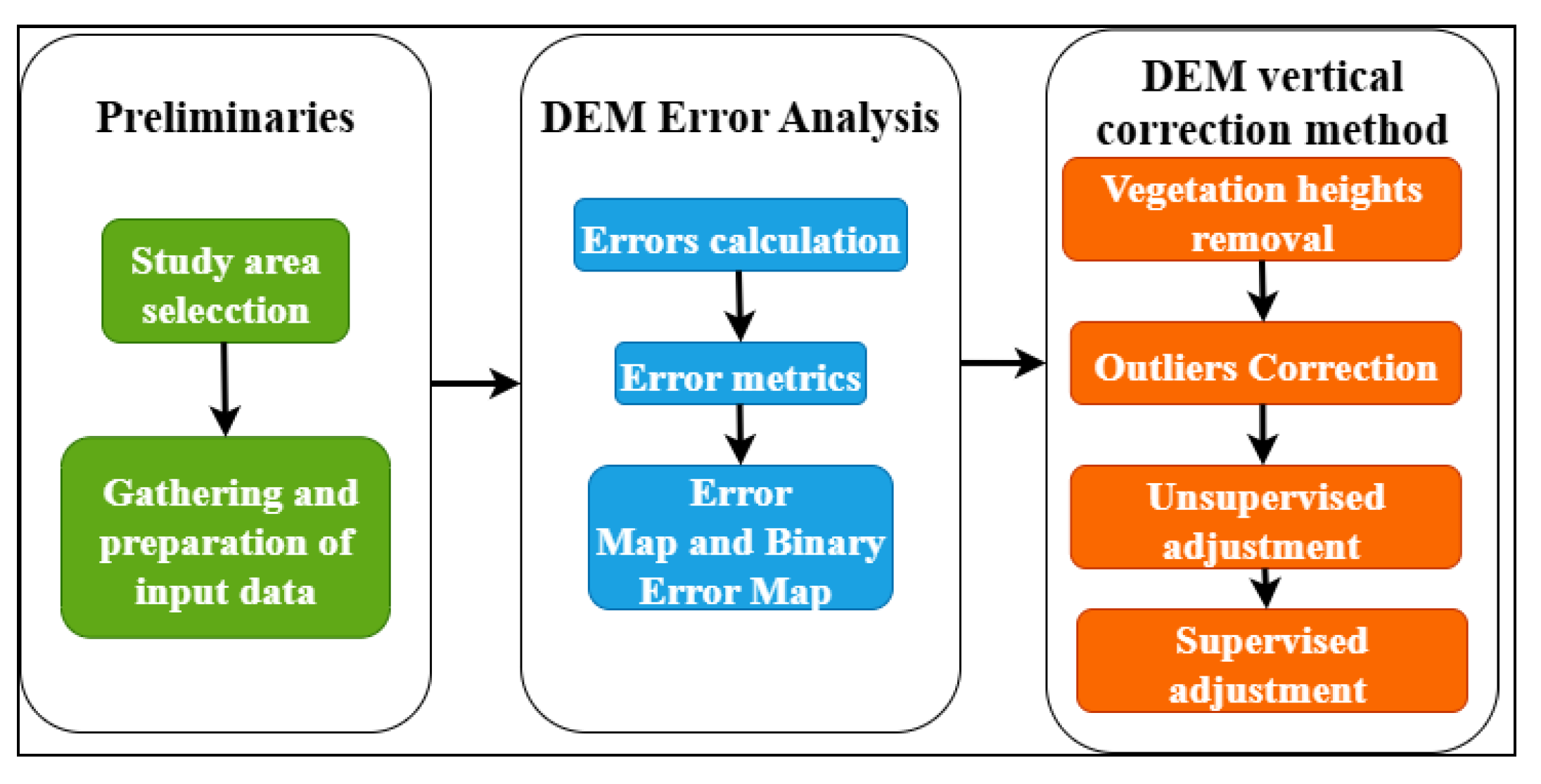
Figure 2.
Unsupervised DEM adjustment
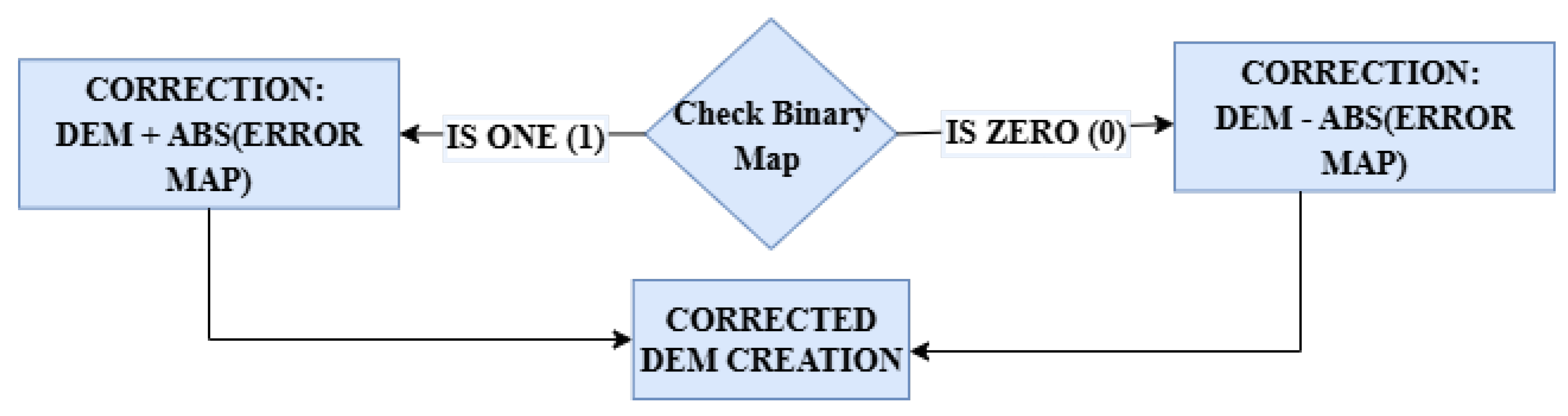
Figure 3.
Location of the Rancheria river delta with respect to the urban area of Riohacha and its discharge to the Caribbean Sea.
Figure 3.
Location of the Rancheria river delta with respect to the urban area of Riohacha and its discharge to the Caribbean Sea.
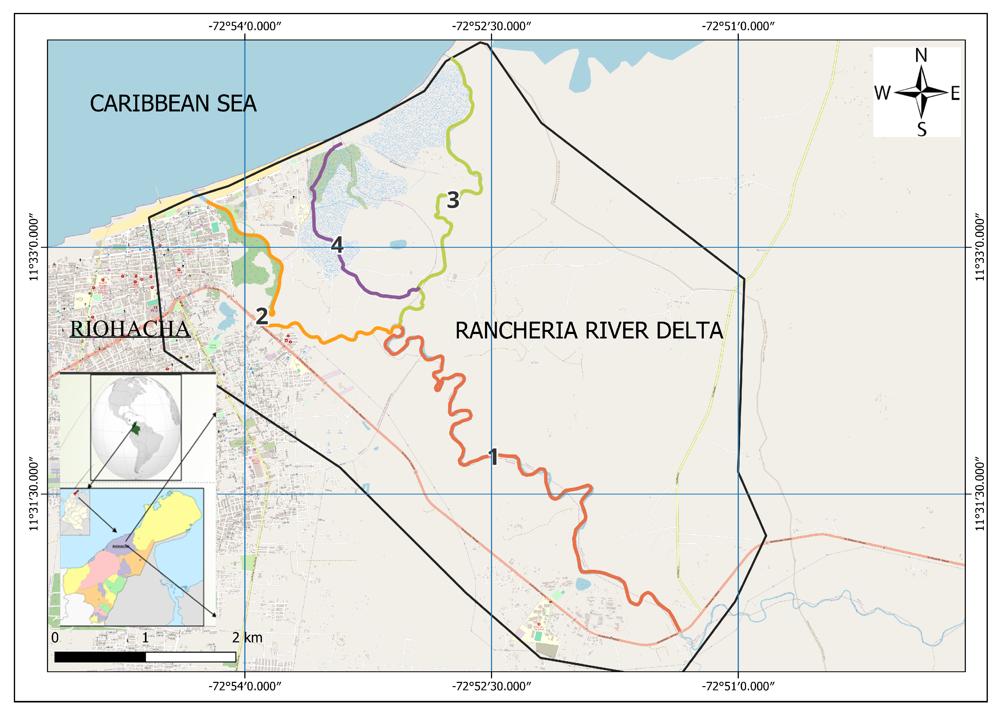
Figure 4.
Used DEMs
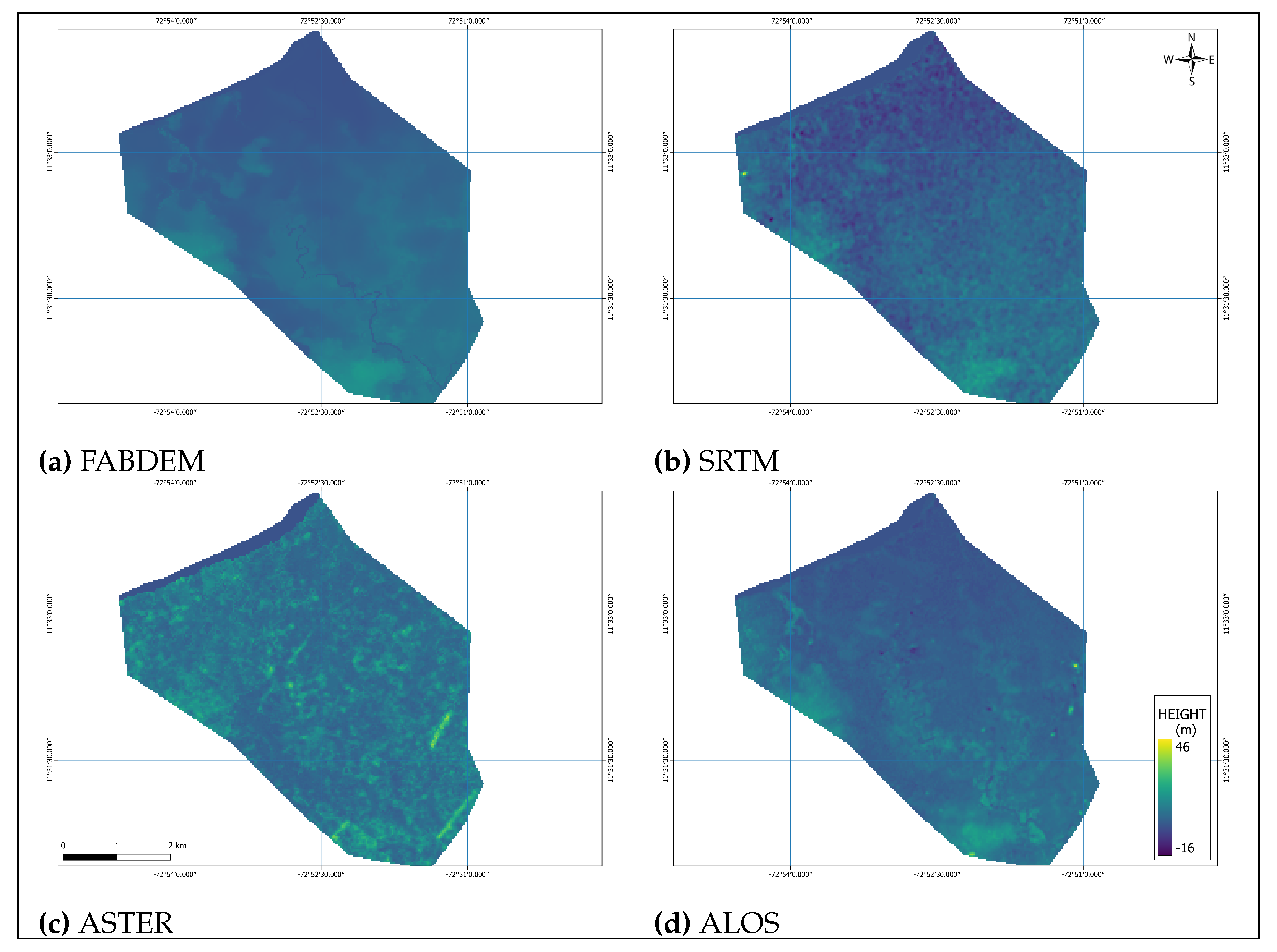
Figure 5.
Land Cover map of the study area.
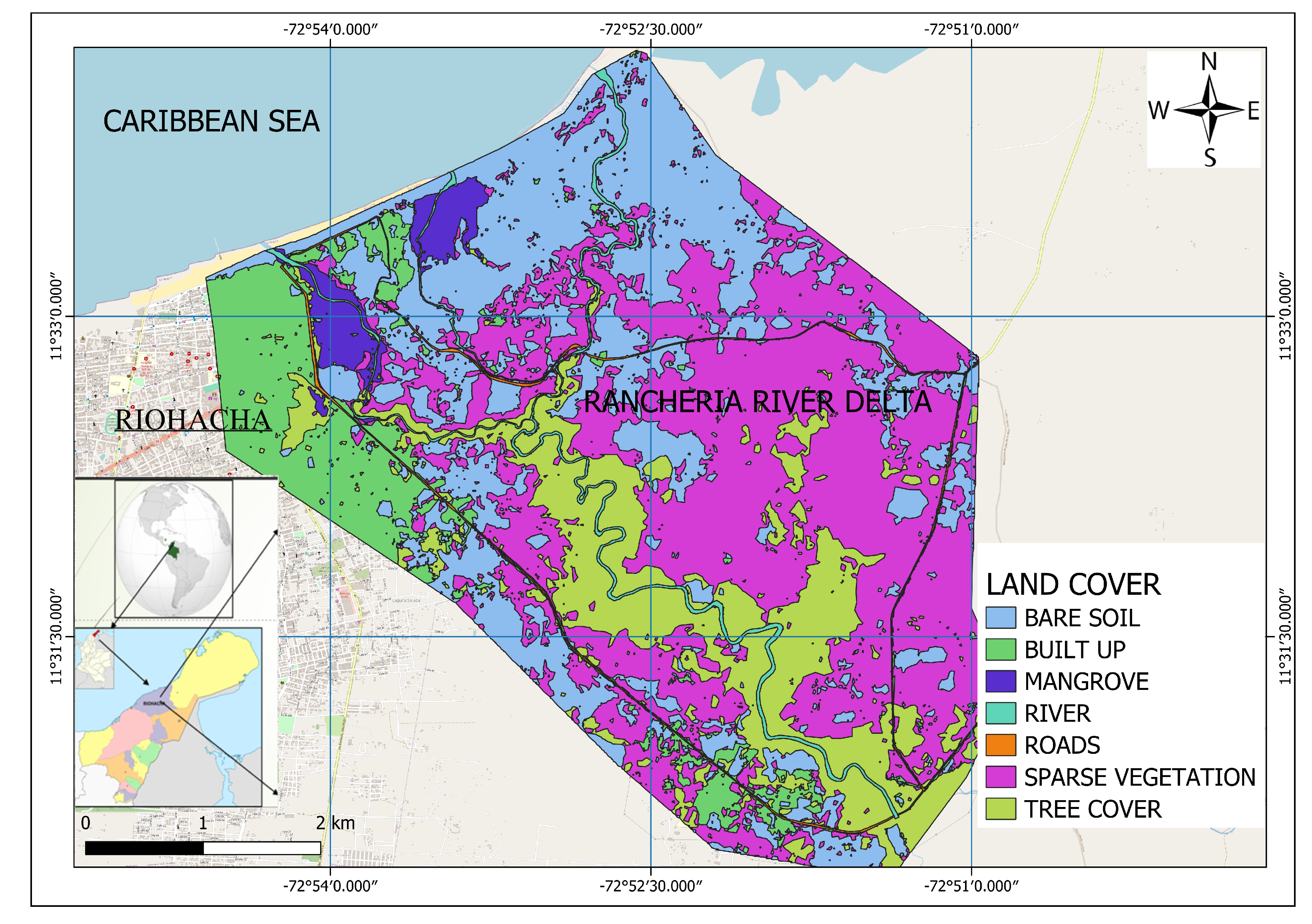
Figure 6.
Canopy Height Model of the study area.
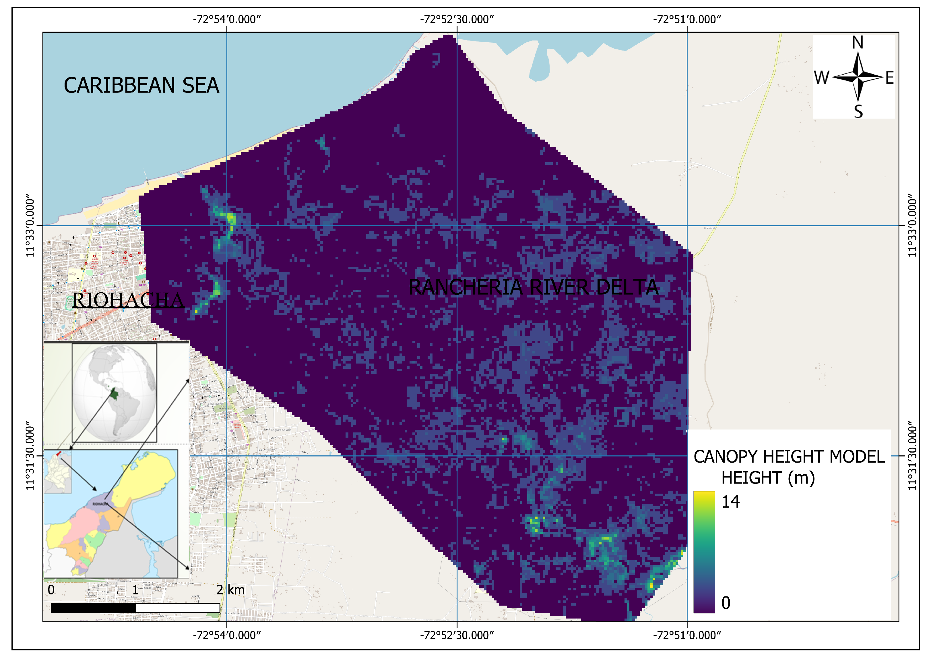
Figure 7.
Topographic points surveyed in the study area.
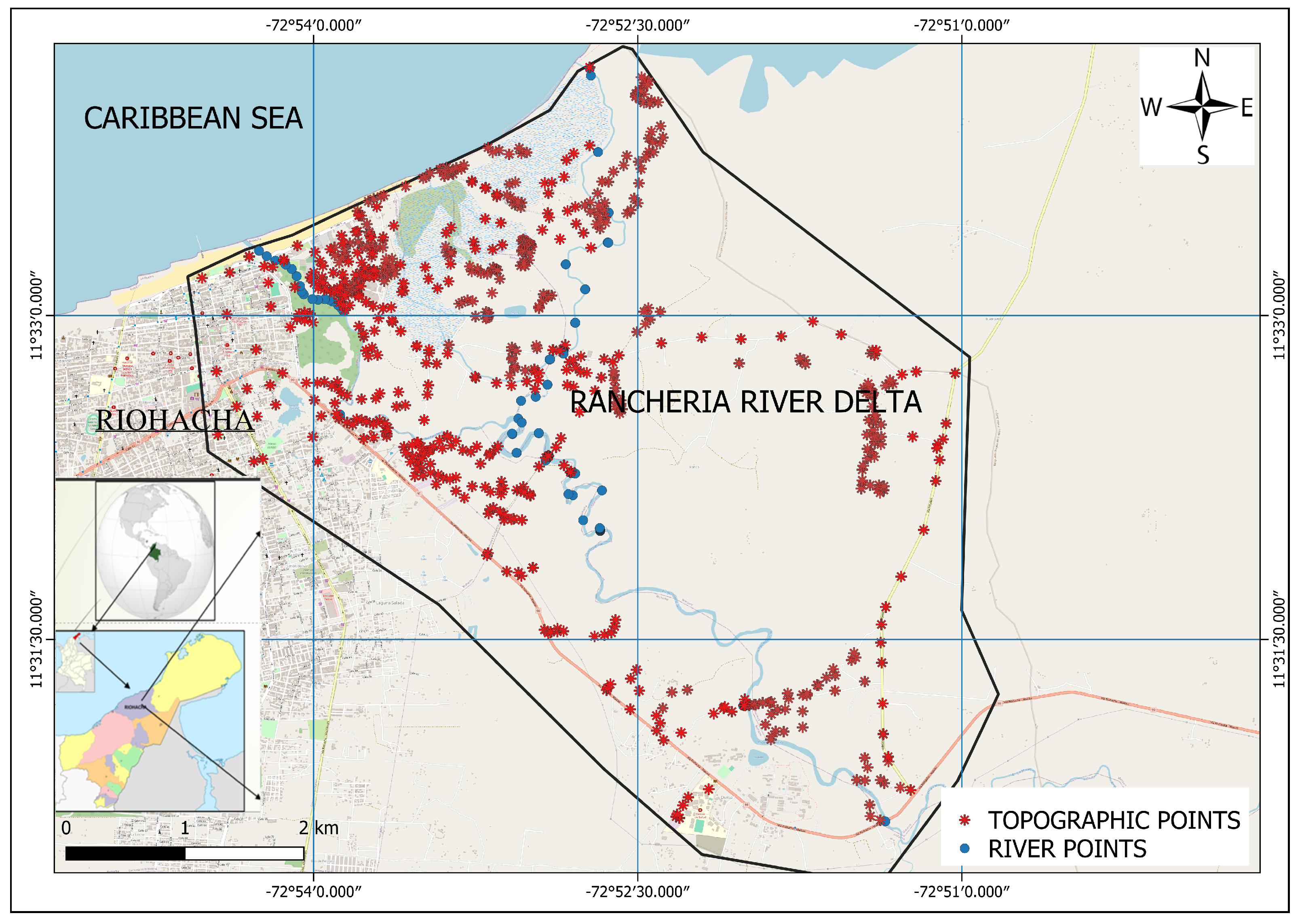
Figure 8.
Error distribution and error metrics
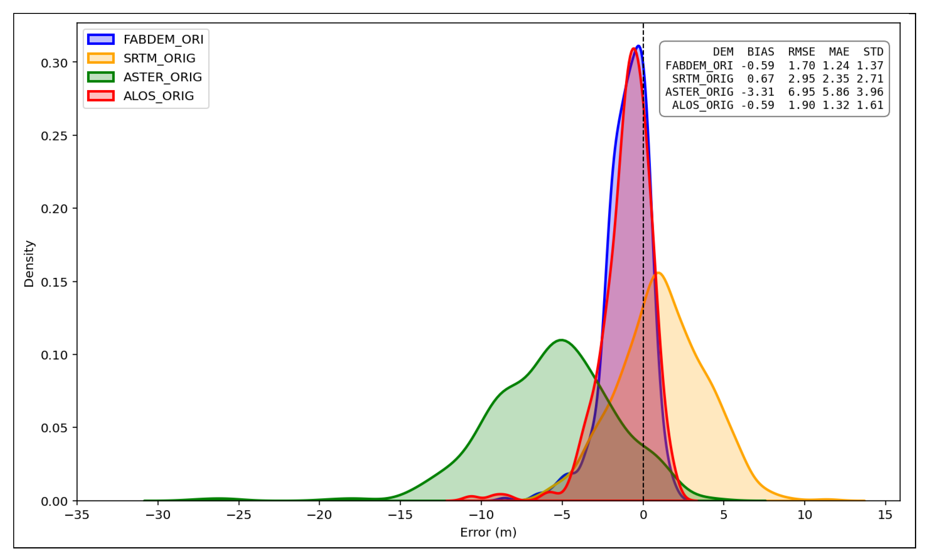
Figure 9.
Error Maps
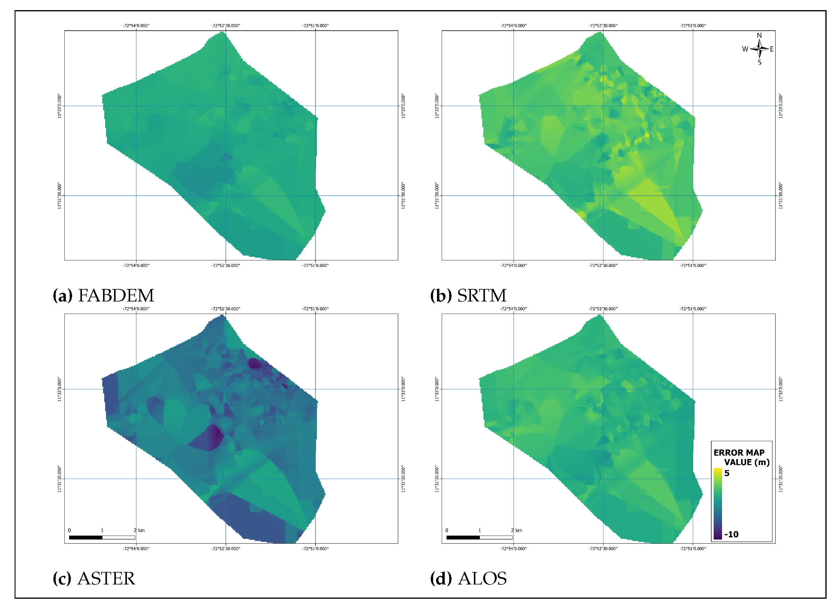
Figure 10.
Binary Error Maps
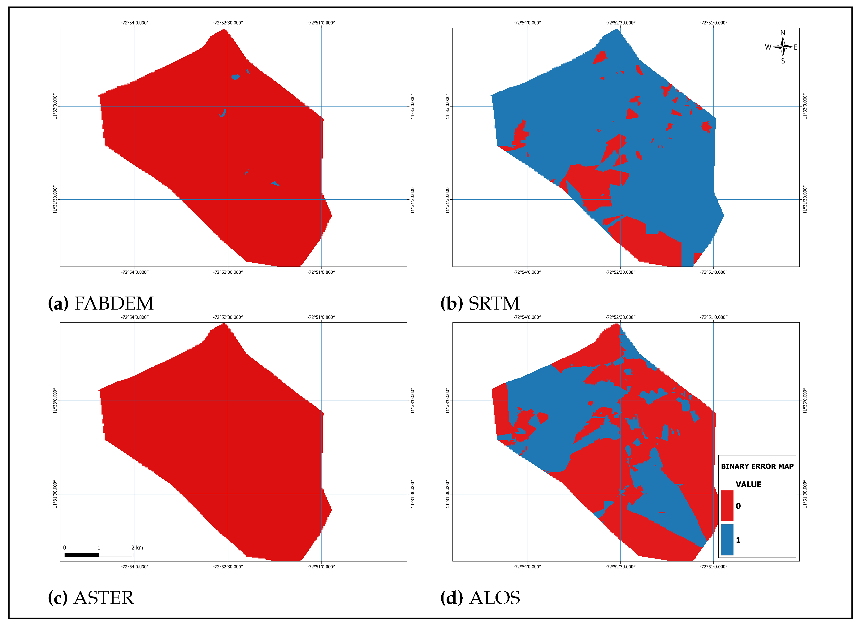
Figure 11.
Comparison of error distribution and metrics before and after applying the correction method
Figure 11.
Comparison of error distribution and metrics before and after applying the correction method
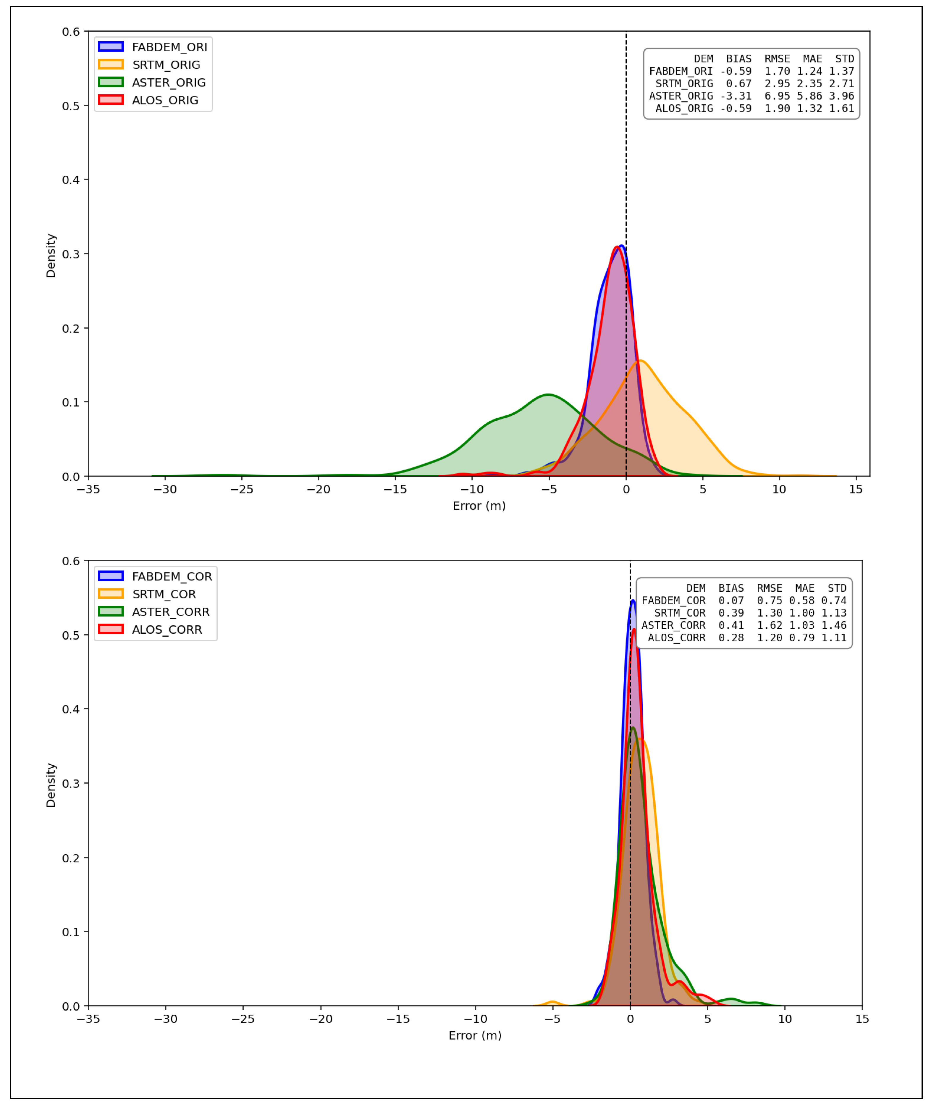
Figure 12.
Comparison box plot graphs, original and corrected DEMs
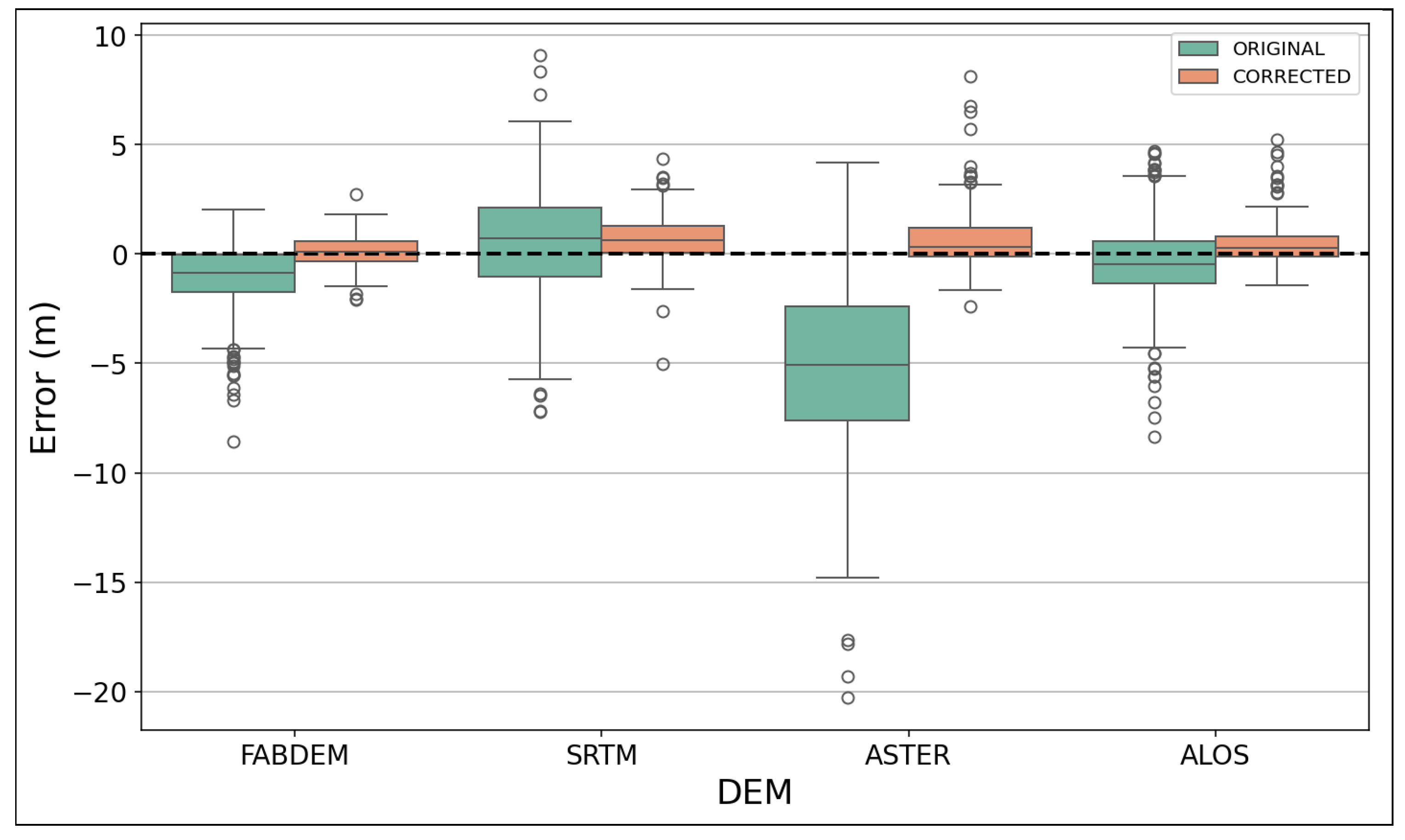
Figure 13.
Altimetrically corrected DEMs
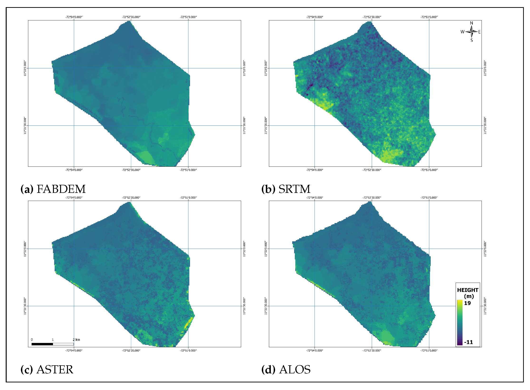
Figure 14.
Profiles to evaluate DEM elevations (Arrow indicates profile’s drawing direction).
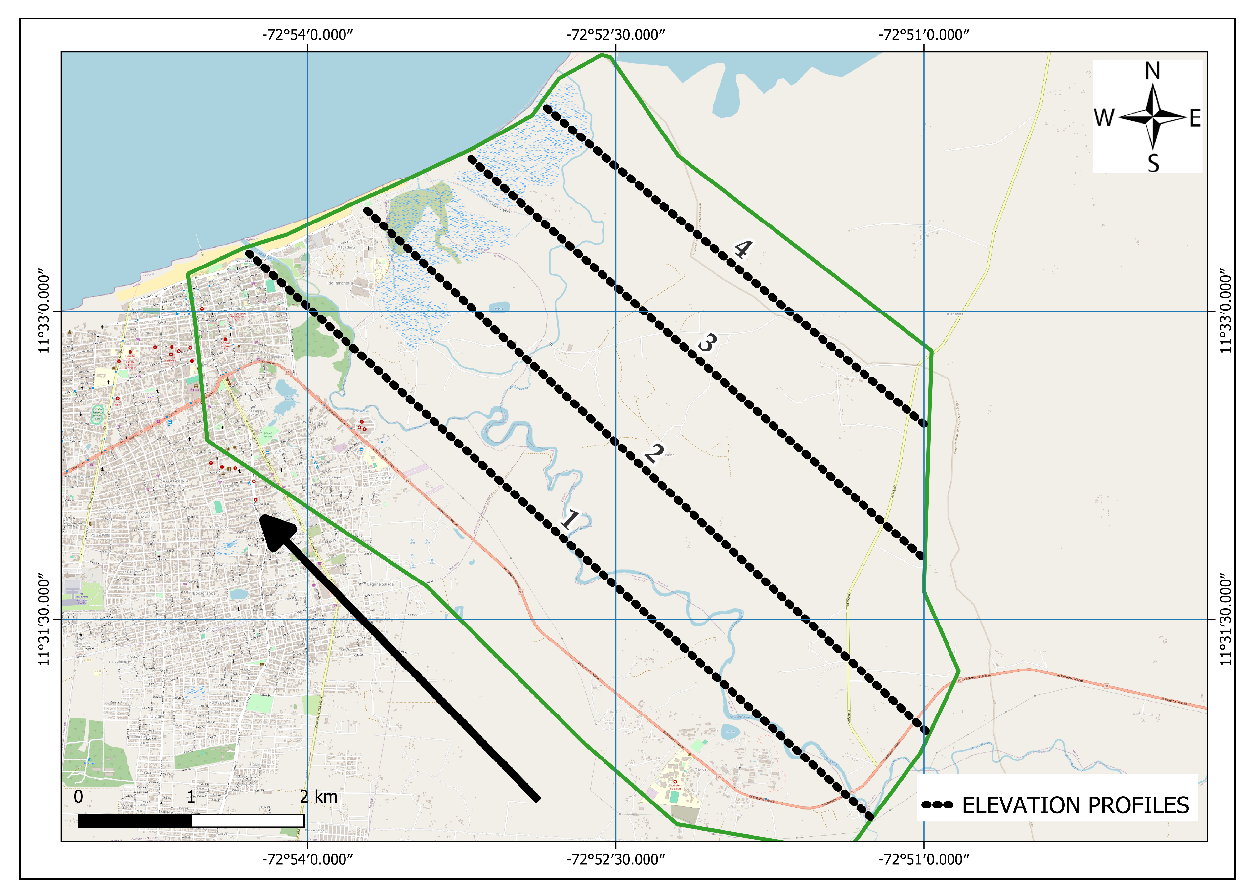
Figure 15.
Comparison of elevation profiles before and after applying the correction method.
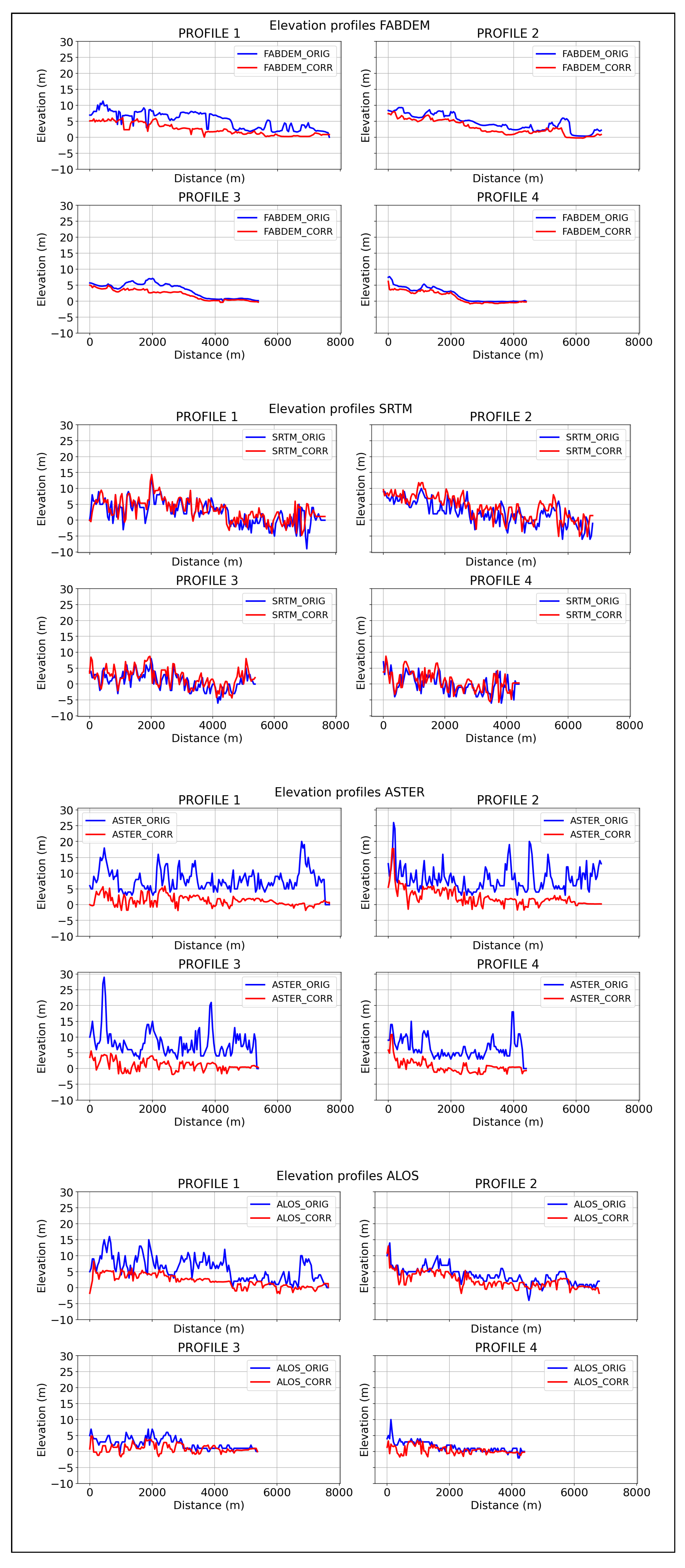
Figure 16.
Comparison profiles between DEMs before and after applying the correction method
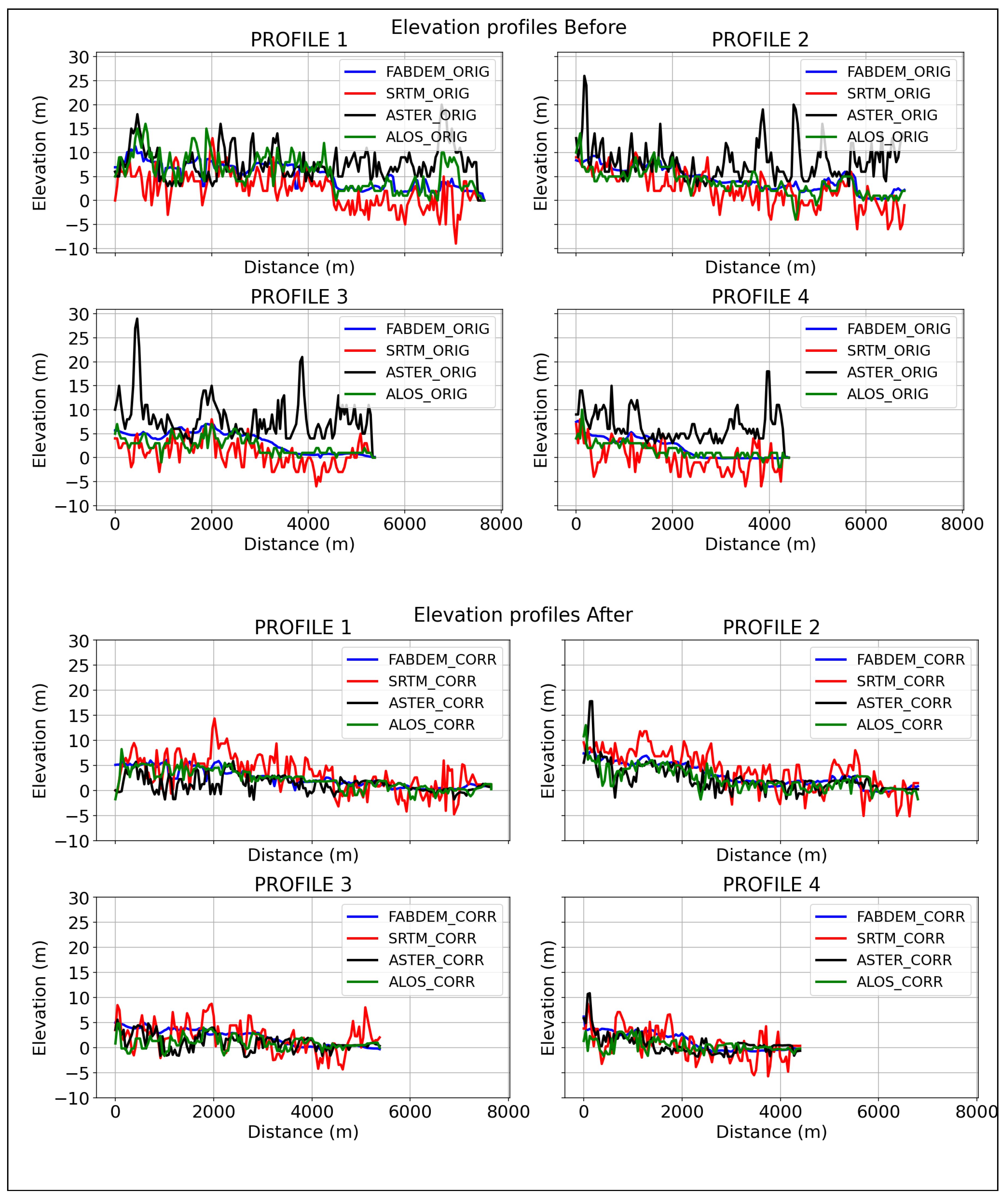

Table 1.
Comparison of metrics before and after applying the correction method. Best values are highlighted in bold.
Table 1.
Comparison of metrics before and after applying the correction method. Best values are highlighted in bold.
| METRIC | DEM | |||||||||||
|---|---|---|---|---|---|---|---|---|---|---|---|---|
| FABDEM | SRTM | ASTER | ALOS | |||||||||
| ORIG | COR | % | ORIG | COR | % | ORIG | COR | % | ORIG | COR | % | |
| RMSE | 1.700 | 0.750 | 55.882 | 2.950 | 1.300 | 55.932 | 6.950 | 1.620 | 76.691 | 1.900 | 1.200 | 36.842 |
| MAE | 1.240 | 0.580 | 53.226 | 2.350 | 1.000 | 57.447 | 5.860 | 1.030 | 82.423 | 1.320 | 0.790 | 40.152 |
| STD | 1.370 | 0.740 | 45.985 | 2.710 | 1.130 | 58.303 | 3.960 | 1.460 | 63.131 | 1.610 | 1.110 | 31.056 |
| BIAS | -0.590 | 0.070 | — | 0.670 | 0.390 | — | -3.310 | 0.410 | — | -0.590 | 0.280 | — |
ORIG: Original; COR: Corrected; Values in % represent the improvement rate after correction. Bold numbers indicate the best performance per metric.
Disclaimer/Publisher’s Note: The statements, opinions and data contained in all publications are solely those of the individual author(s) and contributor(s) and not of MDPI and/or the editor(s). MDPI and/or the editor(s) disclaim responsibility for any injury to people or property resulting from any ideas, methods, instructions or products referred to in the content. |
© 2025 by the authors. Licensee MDPI, Basel, Switzerland. This article is an open access article distributed under the terms and conditions of the Creative Commons Attribution (CC BY) license (http://creativecommons.org/licenses/by/4.0/).
Copyright: This open access article is published under a Creative Commons CC BY 4.0 license, which permit the free download, distribution, and reuse, provided that the author and preprint are cited in any reuse.


