
Submitted:
16 July 2025
Posted:
18 July 2025
You are already at the latest version
Abstract
In this paper a class of fully probabilistic time series models based on Gaussian Vector Mixtures (VMs), i.e., Gaussian multivariate mixtures, is proposed to model electricity Day Ahead Market (DAM) hourly prices and to generate related future scenarios. These models intrinsically allow for organizing data in clusters, their parameters having a simple and clear interpretation in terms of market phenomenology, like spikes and night/day seasonality. Differently from current deep learning models, VMs and the other members of the class discussed in the paper, often seen as just `old style’ machine learning in the machine learning community, are shown to be directly interpretable as a subset of the regime switching autoregressions still currently largely used in the econometric community. The paper can be thought as divided in two parts. In the first part, VMs are estimated and used to model daily vector sequences of 24 prices, thus assessing their scenario generation capability. In this part it is shown that VMs can hierarchically cluster data, can preserve and encode very well intraday dynamic structure like autocorrelation up to 24 lags, but also that they cannot handle interday structure. In the second part, these mixtures are dynamically extended to incorporate features typical of hidden Markov models, thus becoming Vector Hidden Markov Mixtures (VHMMs). VHMMs are shown to be able to model both intraday and interday phenomenology, hence able to include autocorrelation beyond 24 lags. They are also shown to possess enough internal structure to exploit and carry forward hierarchical clustering in their dynamics, their small number of parameters still preserving a simple and clear interpretation in terms of market phenomenology and in terms of standard econometrics. All these properties are thus also available to their regime switching counterparts. In practice, these very simple models are able to learn latent price regimes from historical data in an unsupervised fashion, enabling the generation of realistic market scenarios and also probabilistic forecasts, while maintaining straightforward econometrics-like explanability.
Keywords:
machine learning
; stochastic processes
; nonlinear time series analysis
; electricity markets
MSC: 37M10
1. Introduction
Day-Ahead Markets (DAM) of electricity are markets in which, on each day, prices for the 24 hours of the next day form at once in an auction, usually held at midday. The data obtained from these markets are organized and presented in a discrete hourly time sequence, but actually the 24 prices of each day share the same information. Accurate encoding and synthetic generation of these time series is important not only as a response to a theoretical challenge, but also for the practical purposes of short term price risk management. The most important features of the hourly price sequences are night/day seasonality, casual sudden upward spikes appearing only at daytime, downward spikes appearing at night time, spike clustering, and long memory with respect to previous days. From a modeling point of view, all of this can mean nonlinearity. Different research communities have developed different DAM prices nonlinear modeling and forecasting methods, discussed and neatly classified some time ago in Ref. [1]. Interestingly, in Ref. [1] it is also noted that a large part of papers and models in this research area can be mainly attributed to just two cultures, that of econometricians/statisticians and that of engineers/computational intelligence (CI) people. This bipartition seems to be still valid nowadays. DAM econometricians tend to use discrete time stochastic autoregressions for point forecasting and quantile regressions for probabilistic forecasting [2], whereas DAM CI people prefer to work with machine learning methods, in some cases also fully probabilistic [3,4]. For example, the CI community has adopted so far deep learning techniques both for point forecasting such as recurrent networks (see for example the NBEATSx model [5,6] applied to DAM data), and for probabilistic forecasting like conditional GANs [7,8,9] and normalizing flows. In addition, there exist deep learning forecasting models which were never tested on DAM price forecasting. For example, the Temporal Fusion Transformer [10] can do probabilistic forecasting characterized by learning temporal relationships at different scales, emphasizing the importance of combining probabilistic accuracy with interpretability. DeepAR [11] is able to predict joint Gaussian distributions (in its DeepVAR form). Noticeably, often these models use the depth dimension for trying to capture multi-scale details (along the day time coordinate and along hours of the same day), at the expense of requiring a very large number of parameters. In their inception, the machine learning methods were often applied to DAM data as black box tools, with a research stance focused mainly on checking whether they work or not on specific data sets. Nowadays internal parts of model architecture are explicitly dedicated to exploiting specific behaviors, like in the NBEATSx model. In any case, this `two-cultures paradigm’ finding, earlier discussed in Ref.[12] for a broader context, is stimulating in itself, because it can orientate further research.
Building on these grounds, this paper, taking the stance of econometrics but still making use of `old style’, shallow machine learning, will discuss the use of the Vector Mixture (VM) and Vector Hidden Markov Mixture (VHMM) family of models in the context of DAM prices modeling and scenario generation. This family of models is usually approached by the econometrics and CI communities with two different formalisms, so that it can misleadingly appear from the two perspectives as two different families. The VM/VHMM family is based on Gaussian mixtures and hidden Markov models, well known in machine learning [13], where it is studied using a fully probabilistic approach [14]. In this paper it will be shown that the members of this family correspond to the Gaussian regime switching 0-lag vector autoregressions of standard econometrics, studied instead using a stochastic difference equations approach. Actually, already at a first inspection VMs/VHMMs and regime switching autoregressions should suggest that they share some features. They are both based on latent (that is, hidden) variables, and are both intrinsically nonlinear. Moreover, it will be shown that they too can exploit a depth dimension which can be very useful for modeling important details of the data. Being vector models they both can remove fake memory effects from hourly time series by directly modeling them as vector series. Yet, there are also common properties that are usually ascribed to the machine learning side only. For example, it is known that because VMs and VHMMs can do unsupervised deep learning (which however current deep learning models usually don’t do), they can automatically organize time series information in a hierarchical and transparent way, which for DAMs lends itself to direct market interpretation. Being VM and VHMM models generative [15], the synthetic series which they produce automatically include many of the features and fine details present in time series. VMs and VHMMs can do probabilistic forecasting almost by definition. Yet, these features are not usually ascribed to the regime switching 0-lag vector autoregression models too. VMs and VHMMs have also features, knowingly shared by regime switching 0-lag vector autoregressions, which usually are not liked by econometricians. Being generative models, they are not based on errors (i.e. innovations) unlike non-zero lag autoregressions and other discriminative models for time series [16], so that cross-validation, residual analysis and direct comparison with standard autoregressions is not easy. Moreover, being generative and based on hidden states, the way they forecast is different from usual non-zero lag autoregression forecasting. It can be thus interesting and useful to work out in detail these common properties hidden behind the two different formalisms adopted by the two communities, keeping also in mind that to linear econometric models the issue of interpretability is not usually attributed. It can also be interesting to try to understand how these common properties can be profitably used in DAM prices scenario generation and analysis.
Thus, this paper has three aims. First, it will discuss both the VM and VHMM approach to DAM series and how to include an important hierarchical structure in the VM and VHMM models. Second, it will study their behavior on a freely downloadable specific DAM prices data set1 coming from the DAM of Alberta in Canada. In the basic Gaussian form in which it will be presented in this paper, the VM/VHMM approach works with stochastic variables with support on the full real line, so that this approach can be directly applied to series which allow for both negative and positive values. Yet, since in the paper the approach will be tested on one year of prices from the Alberta DAM ( values), which are positive and capped, logprices will be everywhere used instead of prices. Estimation of VM/VHMM models relies on sophisticated and efficient algorithms like the Expectation-Maximization, Baum-Welch and Viterbi algorithms. Some software packages exist to facilitate estimation. The two very good open source free Matlab packages BNT and pmtk3 by K. Murphy [17] were used for many of the computations of this paper. In alternative, one can also use pomegranate [18], a package written in Python. Third, it will try to narrow the gap between the two research communities, by exploring a model class which can be placed at the intersection among those used by the two communities. In the end, these very simple models will be shown to be able to learn latent price regimes from historical data in a highly structured and unsupervised fashion, enabling the generation of realistic market scenarios and also probabilistic forecasts, while maintaining straightforward econometrics-like explainability.
The paper can be thought as being made up by two parts. After this Introduction, Section 2 will define suitable notation and review usual vector autoregression modeling to prepare the discussion on VMs and VHMMs for DAM prices. Section 3 will introduce VMs as machine learning dynamical mixture systems uncorrelated in interday dynamics but correlated in intraday dynamics, and will discuss their inherent capacity of doing clustering. Section 4 will discuss VMs as regime switching models, i.e. as econometric models. It will also show how they can be made deeper, that is, hierarchical. This feature will come especially at hand when they will be extended into VHMMs in a parsimonious way in terms of number of parameters. Section 5 will very briefly discuss forecasting with VMs. Section 6 will show the behavior of VMs when applied to Alberta DAM data in terms of clustering, interpretation of parameters, and scenario generation ability. Section 2 to Section 6 will make up the first part of the paper. Section 7 will introduce VHMMs as models fully correlated in both intraday and interday dynamics, and will discuss their deep learning structure. Section 8 will briefly discuss forecasting with VHMMs. Section 9 will show the behavior of VHMMs when applied to Alberta DAM data, their better scenario generation ability in comparison to VMs, and their special ability of modeling spike clustering. Section 7 to Section 9 will make up the second part of the paper. Section 10 will conclude.
2. Notation and Generative vs. Discriminative Autoregression Modeling
This Section will define suitable notation and review usual vector modeling. This will help putting in context related literature and to prepare the discussion on vector mixtures and Markov models of the following Sections.
Consider the DAM equispaced hourly sample time series of values , where t indicates a given hour starting from the beginning of the sample. In order to link the following discussion with the Alberta data, in what follows will be assumed to be logprices. In DAMs the next day 24 logprices form at once on each day and share the same information, so that it makes microeconomic sense to regroup the hourly scalar series into a daily vector sample series of N days, where the vectors have 24 coordinates each obtained from by the mapping , and are labeled by the day index d and the day’s hour h. The series can be thought as having been sampled from a stochastic chain of vector stochastic variables modeled as the vector autoregression
In Eq. (1) d labels the current day (at which the future at day is uncertain), is a day-independent vector function with hourly components that characterizes the structure of the autoregression model, labels a set of lagged regressors of where
is the number of present plus past days on which day is regressed, with the convention that for
no variables appear in . The earliest day in is hence , so that for example for only is used as a regressor (i.e. 24 hours) and, for , both and (i.e. 48 hours) are used. Hence the autoregression in Eq. (1) uses
vector stochastic variables in all, which include the variable. For , i.e. , Eq. (1) thus represents a 0-lag autoregression. In Eq. (1) represents the set of model parameters. Moreover, in Eq. (1) represents the member at time of a daily vector stochastic chain of i.i.d. vector innovations with coordinates related to days and hours. By definition the vector stochastic variables have their marginal (w.r.t. daily coordinates d) joint (w.r.t. intraday coordinates h) density distributions all equal to a fixed . This will be chosen as a 24-variate Gaussian distribution , where and are (vector) mean and (matrix) covariance of the distribution. Thus in this vector notation can represent also one N-variate (in the daily sense) draw from the chain , driven by a i.i.d. Gaussian noise which yet includes intraday structure. Incidentally, it can be noticed that the model in Eq. (1) includes for a suitable form of the possibility of regressing one day’s hour on the same hour (only) of past days, i.e. independently from other hours as
where are now scalar stochastic variables and , an approach occasionally used in the literature. Seen as a restriction of Eq. (1), this `independent hours’ scalar model is easier to handle than the full vector model of Eq. (1), but it is of course less accurate. In contrast, the full vector model can take into account both intraday and interday dependencies, and allows for a complete panel analysis of data, cross-sectional and longitudinal, coherent with the microeconomic mechanism which generates the data. Commonly used forms of are those linear in most of the parameters, like where are the matrices of coefficients and is a vector nonlinear function. If is linear in the as well, a vector AR() model (VAR()) is obtained, like for example the Gaussian VAR(1) model
For VAR() models the Box-Jenkins model selection procedure can be used to select optimal and to estimate the coefficients.
In the literature, it is however univariate (i.e. scalar) autoregressions directly on the hourly series [19,20], more or less nonlinear and complicated [21,22], which are applied most often. Noticeably, the information structure implicitly assumed by univariate models is the typical causal chain in which prices at hour h depend only on prices of previous hours. On one hand researchers are aware that this structure doesn’t correspond to typical DAM prices information structure [23], but on the other hand vector models are often considered impractical and heavier to estimate and discuss, especially before the arrival of large neural network models. This issue led first to estimate the data as 24 concurrent but independent series like in Eq. (2), then to the introduction of vector linear autoregressions like that in Eq. (3) [24], maybe using non-Gaussian disturbances distributions like in [25] (in this case multivariate Student’s distributions). In the case of models like the VAR(1) of Eq. (3), for each of the lags a matrix of parameters (besides vector means and matrix covariances of the innovations) has to be estimated and interpreted. Adding lags is thus computationally expensive and makes the interpretation of the model more complicated, and weakens stability, but in contrast few lags imply short term memory in term of days, i.e. quickly decaying autocorrelation. Seasonality and nonlinearity (like fractional integration) can be further added to these vector regressions [26], making them able to sustain a longer term memory. A parallel line of research which uses a regime switching type of nonlinearity in the scalar autoregression setting (discussed at length in [27]) does not concentrate on long term memory but can result in an even more satisfactorily modeling of many DAMs key phenomena like concurrent day/night seasonality and price spiking.
Point forecasting is straightforward with vector models in the form of Eq. (1) as
where represents the estimated parameter set. In turn, Eq. (4) allows for defining (conditional) forecast vector errors as
on which scalar error functions can be defined.
As to probabilistic forecasting, it should be noted that the function in Eq. (1) induces a relationship between and that can be written as a conditional distribution
Besides by using stochastic equations like Eq. (1), vector autoregression models can thus also be directly defined by assuming a basic conditional probability distribution like that in Eq. (6). When based on a distribution conditional on some of their variables, probabilistic models are called discriminative.
In contrast, when defined by means of the full joint distribution like
probabilistic models are called generative [28,29,30]. The relationship in Eq. (6), often obtained only numerically, can be used for probabilistic forecasting.
Notice that in the 0-lag case, i.e. for , the set is empty, and Eq. (1) becomes the Gaussian VAR(0) model
(where a possible constant is omitted). The corresponding probabilistic version of this model, i.e. Eq. (6) specialized according to Eq. (8), becomes the product of factors
In this case the defining distribution is unconditional, and the probabilistic model is both of discriminative and generative type. Estimation becomes probability density estimation. The point forecast becomes equal to at all days. Probabilistic forecasting is the distribution itself. Both point and probabilistic out-of-sample forecasts are unconditional and based on past values of variables only in the sense that past values shape the distribution during the estimate phase. More in general, in a generative model errors cannot even be defined, and the Box-Jenkins model selection and estimation procedure, which relies on errors, cannot be applied. Notice that in the generative case a sample from the modeled chain includes variables only, neither more or less, differently from the discriminative case. Generative models are clearly different from discriminative models, and this is probably why their are seldom considered by econometricians.
Finally, it is interesting to compare the realized dynamics for N days implied by probabilistic discriminative models like that in Eq. (6) with the dynamics implied by the VAR(0) model in Eq. (9). Whereas in the former, at each given day d, the next day vector is obtained by sampling from a marginal distribution that changes each day, obtained by feeding the last sampled value back to the distribution, in the latter the sampled distribution never changes. The VAR(0) model is uncorrelated from the point of view of interday dynamics, whereas it remains correlated in intraday dynamics. In contrast, in the case of the generic generative model of Eq. (7), both intraday structure and interday dynamics can be interesting. Based on this point of view, generative models that originate factorized dynamics (like the VAR(0) model and the mixtures which will be introduced next) will be henceforth called uncorrelated, whereas generative models which interday dynamics is more interesting (like the VHMMs) will be called correlated. It will be shown that both types, uncorrelated and correlated, can be in any case very useful for DAM market modeling.
3. Uncorrelated Generative Vector Models, VMs and Clustering
By Eq. (9) the VAR(0) model is defined in distribution as . Estimation of this model on the data set means estimating a multivariate Gaussian distribution with mean vector of coordinates and symmetric covariance matrix of coordinates . Parameter estimation is made by maximizing the likelihood L obtained multiplying Eq. (9) N times, or maximizing the associated loglikelihood LL. The parameters can be thus be obtained analytically from the data, and since the problem is convex this solution is unique. Once has been estimated, estimated `hourly’ univariate marginals and `bi-hourly’ bivariate marginals can be analytically obtained by partial integration of the distribution. In addition, for a generic market day, i.e. a vector , and can define a distance measure in a 24 dimensions space from to the center of the Gaussian of Eq. (9) as
where the superscript indicates the inverse and the superscript ′ indicates the transpose. is called Mahalanobis distance [31]. This measure will be used later.
The VAR(0) model can become a new stochastic chain after replacing its driving Gaussian distribution with a driving Gaussian mixture, i.e., after changing its innovations sector, making it more complex, i.e., a VM. An S-component VM is thus a generative dynamic model defined in distribution as
where is an abbreviated notation for [32]. The S extra parameters subject to are called mixing parameters or weights. Like the VAR(0), the VM is a probabilistic generative model, of 0-lag type, uncorrelated in the sense that it generates an interday independent dynamics, unlimited with respect to maximum attainable sequence length. In Eq. (11) the subscript is there to remark its dynamic nature, since mixture models are not commonly used for stochastic chain modeling, except possibly in GARCH modeling (see for example [33]). A VAR(0) model can thus be seen as a one-component VM. For the distribution in Eq. (11) is multimodal, and maximization of the LL can be made in a numeric way only, either by Montecarlo sampling or by the Expectation-Maximization (EM) algorithm [15,34]. Since EM can get stuck into local minima, multiple EM runs have to be run from varied initial conditions in order to be sure to have reached the global minimum. Means and covariances of the S-component VM can be computed in an analytic way from means and covariances of the components. For example, in the case in the vector notation the mean is
and in coordinates the covariance is
Hourly variance is obtained for in terms of component hourly variances and as
The mixture hourly variance is thus the weighted sum of component variances plus a correction term which is similar to covariance in the case of a weighted sum of two gaussian variables. Based on the component variances, in analogy with the distance defined in Eq. (10) a number S of Mahalanobis distances can be now associated to each data vector . In Eq. (11) the weights can be interpreted as probabilities of a discrete hidden variable s, i.e., as a distribution over s.
An estimated VM implicitly clusters data, in a probabilistic way. In machine learning, clustering, i.e., unsupervised classification of vector data points called evidences into a predefined number K of classes, can be made in either a deterministic or a probabilistic way. Deterministic clustering is obtained using algorithms like K-means [35], based on the notion of distance between two vectors. K-means generates K optimal vectors called centroids and partitions the evidences into K groups such that each evidence is classified as belonging only to the group (cluster) corresponding to the nearest centroid in a yes/not way. Here `near’ is used in the sense of a chosen distance measure, often called linkage. In this paper, for the K-means analysis used in the Figures the Euclidean distance linkage is used. Probabilistic clustering into clusters can be obtained using S-component mixtures in the following way. In a first step the estimation of a S-component mixture on all evidences finds the best placement of means and covariances of S component distributions, in addition to S weights , seen as unconditional probabilities . Here best is intended in terms of maximum likelihood. The component means are vectors that can be interpreted as centroids, the covariances can be interpreted as parts of distance measures from the centroids, in the Mahalanobis linkage sense of Eq. (10). In a second step, centroids are kept fixed. Conditional probabilities called responsibilities are then computed by means of a Bayesian-like inference approach which uses a single-point likelihood. In this way, to each evidence a probability of belonging to one of the clusters is associated, a member relationship which is softer than the yes/not membership given by K-means. For this reason, K-means clustering is called hard clustering, and probabilistic clustering is called soft clustering. Being a mixture, an uncorrelated VM model can do soft clustering in a intrinsic way.
4. VMs as Hierarchical Regime Switching Models
In a dynamical setting, independent copies of the mixture variable s can be associated to the days, thus forming a (scalar) stochastic chain ancillary to . This suggests an econometric interpretation of VMs. Consider as an example the model. Each draw at day d from the two-component VM can be seen as a hierarchical two-step (i.e., doubly stochastic) process, which consists of the following sequence. At first, flip a Bernoulli coin represented by the scalar stochastic variable with support and probabilities . Then, draw from (only) one of the two stochastic variables , , specifically from the one which i corresponds to the outcome of the Bernoulli flip. The variables are chosen independent from each other and distributed as . If is the support of , the VM can thus be seen as the stochastic nonlinear time series
a vector Gaussian regime switching model in the time coordinate d, where the regimes 1 and 2 are formally autoregressions without lags, i.e., of VAR(0) form. A path of length N generated by this model consists of a sequence of N hierarchical sampling acts from Eq. (15), which is called ancestor sampling. In Eq. (15) the r.h.s. variables , , are daily innovations (i.e., noise generators) and the l.h.s. variables , are system dynamic variables. Even though the value of is hidden and unobserved, it does have an effect on the outcome of observed because of Eq. (15). Notice that if the regimes had , for example like the VAR(1) model of Eq. (3), the model would have been discriminative and not generative. It would have had a probabilistic structure based on the conditional distribution , like most regime switching models used in the literature [20]. Yet, it wouldn’t be capable to do soft clustering.
Generative modeling requires at first to choose the joint distribution. The hierarchical structure interpretation of Eq. (15) implies that in this case the generative modeling joint distribution is chosen as the product of factors of the type
From Eq. (16) the marginal distribution of the observable variables can be obtained by summation
A graphic representation of a VM model is shown in Figure 1, where model probabilistic dependency structure is shown in such a way that the dynamic stochastic variables, like those appearing on the l.h.s. of Eq. (15), are encircled in shaded (observable type) and unshaded (unobservable type) circles, and linked by an arrow that goes from the conditioning to the conditioned variable. This structure is typical of Bayes Networks [15]. Specifically, in panel a) of Figure 1 the model of Eq. (15) is shown.
It will be now shown that models like that in Figure 1 a) can be made deeper, like those Figure 1 b) and c), and that this form is also necessary for a parsimonious form of modeling in VHMMs to be discussed in Sec.Section 7. Define the depth of a dynamic VM as the number J of hidden variable layers plus one, counting in the layer as the first of the hierarchy. A deep VM can be defined as a VM with , i.e., with more than two layers in all, in contrast with the shallow (using machine learning terminology) VM of Eq. (15). A deep VM is a hierarchical VM, that can be also used to detect cluster-within-clusters structures.
As an example, a VM can be defined in the following way. For a given day d, let and to be again two scalar stochastic variables with S-valued integer support , and same distribution . Let to be S new scalar stochastic variables, all with same M-valued integer support , , and with time-independent distributions . Consider the following VM obtained for and :
where
In Eq. (18) the second layer variables are thus described by conditional distributions . This is a regime switching chain which switches among four different VAR(0) autoregressions. Seen the model as a cascade chain, at time , a Bernoulli coin is flipped at first. This first flip assigns a value to . After this flip, one out of a set of two other Bernoulli coins is flipped in turn, either or , its choice being conditional on the first coin outcome. This second flip assigns a value to . Finally, one Gaussian out of four is chosen conditional on the outcomes of both the first and the second flip. Momentarily dropping for clarity the subscript from the dynamic variables and reversing to mixture notation, the observable sector of this partially hidden hierarchical system is expressed in distribution as a (marginal) distribution in , with a double sum on hidden component sub-distribution indexes
The number of components used in Eq. (20) is . Notice again that the Gaussians are here conditioned on both second and third hierarchical layer i and j indices. See panel b) of Figure 1 for a graphical description. Intermediate layer information about the discrete distributions can be collected in a matrix
which supplements the piece of information contained in . In this notation Eq. (20) becomes
Notice also that this hierarchical structure is more flexible than writing the same system as a shallow flip of an faces dice, because it fully exposes all possible conditionalities present in the chain, better represents hierarchical clustering, and allows for asymmetries - like having one cluster with two subclusters inside and another cluster without internal subclusters. In addition to the structure of Eq. (18), another more compact hierarchical structure, a useful special case of Eq. (18), is
with the same f as in Eq. (19). This system has distribution (in the simplified notation)
or, for ,
where and , and where now the Gaussians are conditioned to the next layer only. See panel c) of Figure 1 for a graphical description. This chain can also model a situation in which two different mixtures of the same pair of Gaussians are drawn. In this case each state corresponds to a bimodal distribution , unlike the shallow model. This structure, which is a three-layer two-component regime switching dynamics from an econometric point of view, will be specifically used later when discussing hidden Markov mixtures.
5. VMs and Forecasting
With VMs, a possible point forecast at day d can be obtained by the use of estimated means. For example, in the case of the model of Eq. (18), using the indexed symbol for the vector mean of the conditional Gaussian , for its estimate, and for the forecast value, from Eq. (22) one obtains
This 24-hours-ahead point forecast cannot go beyond forecasting the same hourly profile at any day. Notice that Eq. (26) can also be used to form makeshift daily errors of the type .
Besides point forecasting, deep VMs can of course do deep volatility forecasting, through combinations of conditional covariances , and more complete probabilistic forecasting like quantile or other risk measure forecasting. In the case of a shallow two-component model, the volatility forecast has the form of Eq. (13).
6. Uncorrelated models on data
Before extending the uncorrelated models to correlated models of VHMM type, in this Section it will be discussed some examples of how VMs can extract features from data, and some examples of the scenarios they can generate.
6.1. Alberta DAM Data
The theory discussed in Section 3 and Section 4 will be now applied to the Alberta DAM data. Figure 2 shows one year of Alberta DAM price (in Canadian Dollars, upper panel) and logprice (lower panel) data, i.e., 8670 hourly values reffering to the one-year period from Apr-07-2006 to Apr-06-2007 organized in one sequence. This period was chosen due to the variety of price structures observed, with large jumps and spikes, and the presence of a marked mean-reversion component.
In this year of the Alberta market, only positive prices are allowed, and prices are capped. In the upper panel Figure 2, notice the heavy spiking behavior, which mathematically means strong mean reversion after each spike, and spike clustering. In the lower panel, in which logprices are shown, notice that, besides upward spikes, downward spikes (antispikes) are significantly present (they are magnified by the logarithm). Figure 3 shows a blowup of the full series, two weeks of hourly values, i.e., fourteen individual market data vectors presented in sequence.
Some days are of the spiky type, others are quieter. Notice how spikes appear only during daylight and antispikes appear only during night time, all this due to a sinusoidally time varying demand (see related mathematical discussions in [36,37]). In weekends spikes are less frequent, so that there is a weekly periodicity. Figure 4 shows the same Alberta data, organized in a different way.
The upper panel shows the empirical, unconditional distribution of all logprices in the sample set. Notice that this distribution is not Gaussian, it has thick tails due to spikes and antispikes, and it is skewed to the right since there are more spikes than antispikes (compare with Figure 2). The lower panel shows the sample autocorrelation of logprices, where logprices were preprocessed subtracting at each the corresponding full sample hourly mean
where is the number of samples used. In the autocorrelation, notice the peaks at multiples of 24 hours, due to the daily nature of the auctions, and the little bump at hour 12 and its multiples, due to night/day demand alternation. Notice also the very long slow decaying tail, indicating slow decorrelation among days. Such a long tail implies that autoregressions must include many lags. Figure 5 shows sample histograms of logprice distributions at four fixed hours.
Notice evident multimodality and skewness. Morning hour 1 distribution is rather Gaussian in shape, but other hours like for example peak hours 12 and 18 are not Gaussian at all and at least bimodal. Superimposed to sample distributions, black curves (to be further commented later on), show how a two-component VM can fit these data, and hint at the possibility that mixtures with more components could model them even better. Incidentally notice that in the following analysis, in general, logprice data will be purposely neither detrended or deseasonalized before being used, and Eq. (27) will be used only in relation to autocorrelations.
6.2. Cluster Analysis, Without and With VMs (i.e., Hard and Soft)
Figure 6 shows a choice of four scatterplots of logprices, respectively at hour pairs , , , (i.e., with the first hour fixed at ), where in each panel all pairs in the data set are plot. The dots on these four scatterplots are 2-dimensional projections of points (that is market days) living in the 24 coordinates space. The points tend to lay on the diagonal, i.e., with a positive correlation. A K-means cluster analysis for finds the centroid components of the two clusters (where , indicated on each panel with a cross), for each pair of hours and . Cluster membership of each point is indicated by the light red or dark blue color. Data are rather sharply clustered by the K-means algorithm. One cluster (in the panel south-west sector) contains logprices which are low at hour 1, deep in the night, and stay low at following hours. The other cluster (north-east) contains logprices which are higher and stay higher during the 24 hours. A Variance Ratio analysis [38,39] not reported here graphically, which computes VRS for a sequence of S values for K-means and soft clustering (i.e., using VMs), shows that VRS is maximized by for all three methods. This result quantitatively confirms that the market days can be classified in a clear way into two different types. A Bayes Information Criterion (BIC) analysis gives the same result.
6.3. Estimate of a VM and Its Interpretation
Figure 7 shows a shallow two-component VM fit of the data. Each state in this model corresponds to a unimodal distribution. The upper panel shows the hourly sample means of logprices (solid line), the hours being indicated on the x-axis, each mean bracketed by the related one sample standard deviation interval (the two dotted lines). In practice, the panel shows the average market day, with low logprices during night time and higher logprices during daylight. The lower panel shows the estimated hourly means (solid line) and their one-standard-deviation boundaries (dotted lines), obtained from the vector of Eq. (12) and from the square root of the diagonal elements of the matrix of Eq. (13). The curves are indistinguishable.
Figure 8 shows estimated hourly component means and component standard deviation from , and respective values (). The component hourly means should be compared to the hard clustering information of Figure 6. For example, x-axis value of first cluster’s hour 1 in that Figure has clearly the same value of first component (upper panel of Figure 8), and x-axis value of second cluster’s hour 1 has clearly the same value of second component (lower panel). This means that the two 24-coordinate Gaussians found with the VM soft clustering analysis match well the two 24-coordinate clusters found with the hard clustering exploration, the main difference between the two methods being the type of distance used by VM clustering, which is the Mahalanobis metric of Eq. (10). Notice that looking at the individual profiles of the two components, which have comparable weights , the difference in their hourly standard deviations during daily hours is substantial. Recalling the two-levels interpretation of the shallow two-component VM of Eq. (15), having the two components a similar hourly mean profile but having the second component a much lower variance during daylight, this second component can be interpreted as modeling a sort of nightly logprice pattern, to which the more spiky behavior of the first daylight component very often alternates (because ). A fit of total covariance shows that the sample covariance matrix and the matrix estimated by Eq. (13) practically coincide, as it happened for the means.
More interestingly, Figure 9 shows estimated component covariances . Here the interpretation of the two components in terms of `day vs. night’ becomes even clearer. The first component has a lot of variance along the daylight diagonal portion whereas the second component has none, showing some variance (the greenish square in the upper left corner of the panel) only during night time, that is when antispikes appear. The possibility of this interpretation in terms of abstraction and of representation learning is strictly connected to the use of a generative model like the VM, which allows for both classification and stochastic time series interpretation. In order to clarify what is the criterion with which the VM model classifies vector data, it is better to consider it as a regime switching zero-lag model.
To illustrate this criterion even more pictorially, Figure 10 shows Mahalanobis distances of individual market days from component 1 and component 2 cluster centers (i.e., the two most typical market days selected by the model) in upper and middle panels, and state (i.e., cluster) membership inferred from posterior probability (i.e., responsibilities ) in the lower panel. Large distance from cluster 2 corresponds to large posterior probability of belonging to cluster 1. Market days can be classified ex post in terms of their (hidden) type. Mahalanobis distance, as Eq. (10) shows, exploits all information available from and (i.e., from the cross-sectional structure shown in Figure 8 and Figure 9). Thus, endowing the 24 dimensions market space with two of these distances (which for become the Euclidean distance), similarity among daily patterns is exploited in a very simple, transparent and human-readable way. This richness in information of a two-component model can be directly seen in visualizations that explore daily cross-sectional structure, like Figure 11, where the estimated two-component bivariate marginal distribution is shown (from above) for hours 1 and 12. The probability density function for which the isolevels are plot was obtained analytically, just by evaluating Eq. (11), which consists of the weighted sum of two bivariate Gaussian functions of which all parameters are known. The small circles represent the selected coordinate pairs. Their color shade is obtained first analytically evaluating on each data point the two components with the posterior formula, then associating the daily membership to cluster 1 or cluster 2 by computing
A hard clustering very similar to hard K-means clustering is thus obtained, confirming the day/night interpretation also in terms of what happens at hour 12 to hour 1 logprices. In Figure 11 the two Gaussians have close centers (recall hard cluster positions from Figure 6 and component values from Figure 8), and different peak heights. All of this has obvious potential for accurate scenario generation and for probabilistic forecasting.
Intuition from Figure 11 can be integrated with the results shown in Figure 5, where the solid curves of univariate marginals, analytically obtained, are superimposed to univariate sample distribution histograms. In Figure 5, at hours 12 and 18 the two components’ profiles can be clearly identified, showing that vector generative modeling can deliver accurate analytical information on DAM logprices’ multivariate marginals already with a very small number of components. Three components could do better than two, but a simple shallow two-component modeling requires much less parameters, and can be considered satisfactory enough.
6.4. VM Dynamics and Scenario Generation
Generative models allow for generation of synthetic data by sampling the estimated distribution. In a sense, they take their name from this feature. In the case of DAM vector modeling, each draw represents one market day of 24 hours. Within the dynamic interpretation of an estimated VM, 365 independent draws reorganized in a scalar series of 8670 market hours simulate one market year. In Figure 12, such a synthetic Alberta market year is shown, for prices (upper panel) and logprices (lower panel). Prices show spikes, logprices show spikes and antispikes. The height profile of synthetic spikes is varied, and should be compared with the profile shown in the upper panel of Figure 2. Spike and antispike variability is evident, whereas spike clustering is absent, since each draw (day) is independent from all other draws in the sequence. A blowup of Figure 12, as shown in Figure 13 where only two weeks are shown, is more striking, when compared with Figure 3 where two weeks of market data were shown. The intra-day structure of synthetic prices and logprices displays very clearly the night/day cycle, some days more spiky than others, spikes appearing only during daylight and antispikes appearing during night time, in a casual way. The mechanism behind this great accuracy in the modeling of details is radically different from mechanisms developed in current discrete- and continuous-time models of electricity markets. In multi-component VMs nonlinearity is mainly used for classification and determination of the covariances, and once the right covariances are found, when a component is drawn at the act of sampling, it is the orchestrated interplay among the values of its covariance that generates the daily logprice pattern, in a linear way. Since the components are Gaussian distributions, market configurations distant from cluster centers are exponentially suppressed, so that the model generates only `credible’ (from the model’s point of view) market configurations. In contrast, usual models often use their nonlinearity for growing spikes and forcing mean reversion. In multi-component VMs nonlinearity enters again when fully probabilistic features are modeled, as it was seen in scatterplots, because in that case the marginals are characterized by the full multi-component gaussian structure. For example, the dots on Figure 11 could be a pictorial representation of the 2d projection of 365 draws from the estimated joint distribution, their density being higher near the peaks of the two Gaussians. From a machine learning point of view, a VM learns many details of the daily patterns, then encodes them in a very abstract way in the covariance matrices. Each day thus becomes a lossy reconstruction of the encoded and compressed data set of the Alberta market. This reconstruction is concentrated in the few support values of the hidden dynamics.
Moreover, VM classification into at least two components allows the model to interleave with finely tuned proportions (given by the two mixing weights) `day’ type market days and `night’ type market days (recall from discussion of Eq. (15) that a mixture is not just a weighted sum of Gaussians, but also a sequence of individual components). Figure 14, upper panel, shows the unconditional empirical distribution of all logprices, and has to be compared with upper panel of Figure 4. This panel highlights that the proportions of spikes (right hand tail) and antispikes (left hand tail) are not very well modeled, even though the distribution is correctly skewed to the right (like in the market data, where there are more spikes than antispikes). This distribution too can be found analitically, just summing all 24 gaussian estimated marginal distributions (like those shown in Figure 5) and dividing by 24. The lower panel of Figure 14 shows the autocorrelation function of preprocessed synthetic logprices. Unsurprisingly, there is nonnegligible autocorrelation, but only up to lag 24, that is to one day, even though the VM model includes no lags for itself. Notice also the little night/day demand bump at hour 12, as in Figure 4. These features are due to the vector nature of the model, that never breaks the intraday logprice relationships, in accordance to the DAM nature of the data and the way information is injected in them. What instead the VM model does is breaking the interday relationships, not including any information about preceding days. This is reflected into the lack of autocorrelation beyond lag 24. This mechanism should be contrasted with the scalar autoregression approach which forces spurious autocorrelation inside the estimate, thus generating fake memory.
In sum, the econometric interpretation of VM parameters (means, covariances and weights) in the DAM case is straightforward. In constrast, the econometric interpretation of the estimated coefficients in VAR models is necessarily more vague and very difficult to connect to phenomenological features of series. In a sense, whereas a VM can abstract in a concentrated small number of states, a standard autoregression can’t abstract. Finally, recall also that simple, zero-lag switching autoregressions share with VMs the same modeling features.
6.5. Forecasting
Eq. (26) and the estimate result shown in Figure 7 imply that forecasting with shallow VMs is the same as forecasting by sample averages.
7. Autocorrelated Vector Models and VHMMs
Dynamic econometrics requires models which have a causal temporal structure This is usually automatically enforced by defining them by autoregressions like that in Eq. (1), i.e., in a discriminative way. In fully probabilistic (i.e., generative) modeling such a structure must be directly imposed on the joint distribution which defines the model. One possible approach to enforce a causal structure in a generative model is that of leaving to the hidden dynamics the task of carrying the dynamics forward in time, whereas the observable dynamics is maintained conditionally independent on itself through time. This is what hidden Markov models are designed for [40]. Henceforth, in order to discuss this approach, the symbol for the set of variables will be shortened to . This choice is intended for both keeping notation light and to remark the specific way in which the dynamic generative approach models the variables, that is all at once. In principle, if the data series has N variables, .
A vector Gaussian hidden Markov mixture model is defined in distribution as
for , and
for (i.e., ) [14]. In Equations (29) and (30) is often loosely called prior. In Eq. (29) all will be chosen equal, which makes the system time-homogeneous. The conditional distribution will be instead chosen as a convex combination of Gaussians, as explained in the following. For this system stationarity is defined as that condition in which . A time-homogeneous system which has reached stationarity has hence the property that
for all d, a useful property. It should be yet also recalled out that homogeneity in time doesn’t guarantee stationarity. Notice the overall form of this model, like in the VM case. The observable joint (w.r.t. intraday dynamics) marginal (w.r.t. observable variables) distribution is obtained from Eq. (29) by summing over the support of all , which makes this model a generalized vector mixture. For example, by summing on Eq. (30) one recovers the observable static S-component mixture
used to define the shallow (i.e., not-hierarchical) VM. Since the have a discrete support, it is possible to set up a vector/matrix notation for the daily hidden marginals
and for the constant transition matrix
of entries , where and , with and (columns sum to one). In this notation, for example for , the dynamics of the hidden distribution becomes a multiplicative rule of the form
which starts from an initial distribution . Under A, after n steps forward in time, becomes
where the superscript n on A indicates its n-th power. Time-homogeneous hidden Markov models can be hence be considered `modular’ because, for a given , the hidden dynamics of is completely described by the prior and a single matrix A which repeats itself as a module for times.
This means that, after an estimate on the data, a global A will encode information from all interday transitions, which are local in time. To highlight this feature, sometimes a subscript can be attached to A, like for example .
The number of parameters required for the hidden dynamics of a hidden Markov model is thus in all, usually a small number. To this number, a number of parameters for the observable sector should be added for each state. If Gaussians are used, this number can become very large. Hence, the total number of parameters depends in general mainly on the probabilistic structure of the observable sector of the model. The basic idea behind VHMMs is to take the distribution of the observable dynamics as a vector Gaussian mixture, i.e., to piggyback a VM module onto a hidden Markov dynamics backbone, taking also care not to end up with too many Gaussians. This will allow obtaining correlated dynamic vector generative models which are deep and rich in behavior but at the same time parsimonious in the number of parameters, and which can forecast in a more structured way than VMs.
Consider at first the shallow case in which . In this case, Eq. (29) implies using S Gaussians in all, as many as the states. Ancestor sampling means picking up one of these Gaussians from this fixed set at each time d. This is pictorially represented in panel a) of Figure 15, were one module of the model is shown with two hidden states emitting one Gaussian each. This model is the correlated equivalent of the (uncorrelated) shallow VM of Eq. (15), which was represented in Figure 1 a).
The shallow model can be extended by associating one M-component Gaussian mixture to each of the S hidden states, for S discrete distributions in all, each hidden state thus supporting a vector of M weights and a M-components mixture distribution. This configuration is represented in panel b) of Figure 15, where the two hidden states emit three Gaussians each. The required weight vectors can be gathered into a matrix with non-negative entries, each row of which sums to 1. This is equivalent to using on each day a module of the deep VM of Eq. (18), which was represented in Figure 1 b). This means that corresponds to the matrix W of Eq. (21) and that the Gaussians of this model are conditioned both on the intermediate and on the top layer of the hierarchy. This configuration requires Gaussians in all to be estimated, potentially a lot, each with parameters where , besides A, and .
A more parsimonious model can be obtained by choosing to use M Gaussians instead of . This is obtained by selecting M Gaussians and associating to each of the S hidden states an s-dependent mixture from the fixed pool of these M Gaussians, in a tied way, in the same way as the deep VM of Eq. (23) represented in Figure 1 c) does. Information about the mixtures can be represented by a matrix , formally similar to , but related to a different interpretation. The Gaussians now have form since they are conditioned on the next layer only. This setting is represented in panel c) of Figure 15, where each of the two hidden states is linked to the same triplet of gaussians. Being able to tie a hierarchical mixture is therefore all-important for parsimony, because in the tied case one can have a large number of hidden states but a very small number of Gaussians, maybe two or three, and an overall number of parameters comparable to that of a VAR(1) which has the same memory depth. This last model will be called tied model in contrast with the model with Gaussians, which will be called untied model. The discussed tied model is the smallest model that contains all vector, generative, hidden state features in a fully correlated dynamic way.
From an econometric point of view, the untied and tied VHMM models are deep regime switching VAR(0) autoregressions, with stochastic equations given by Eq. (18) and Eq. (23), where f of Eq. (19) is replaced with
In Eq. (36) is the stochastic matrix associated to the transition matrix A of Eq. (33), i.e., the stochastic generator of the hidden dynamics. Therefore in these models the hidden dynamics evolves according to a linear multiplicative law for the innovations, whereas the overall model results nonlinear. Since the underlying hidden Markov model is modular, it is possible to write in probability density the representative module of these models. For the untied model this module is
having used a mixed notation and having compressed in (i.e., in ) the `static dynamics’ of the , i.e., the parametrization of the intermediate layer. Eq. (37) corresponds to the one-lag regime switching chain of Eq. (18). For the tied model,
where are the entries of , i.e., the piece of information about the intermediate layer. This dynamic probabilistic equation corresponds to the stochastic chain of Eq. (23). Hence, suitable regime switching VAR(0) autoregressions can have all the properties of the generative correlated VHMM models, clustering capabilities included. One could also say that Equations (37) and (38) are the machine learning, vector generative correlatives of the vector discriminative dynamics of Eq. (1), which in contrast has no hidden layers, it is based on additive innovations, and can have . Noticeably, the hidden stochastic variables of the intermediate layer of the untied and tied models don’t have an autonomous dynamics, like has. But, if needed, they can be promoted to have it as well without changing the essential architecture of the models. Moreover, being Markovian, these dynamic models incorporate a one-lag memory, controlled by A. But, if needed, this memory can be in principle extended to more lags, by replacing the first order Markov chain of the hidden dynamics with an higher order Markov chain.
Finally, from a simulation point of view, each draw from these systems will consist of one joint draw of all variables at once. This is typical of generative models. From a more econometric point of view, this one draw can be seen as a sequence of draws from , local in time, each causally dependent on the preceding one only, and with a deep cascading component on their top at each time.
8. VHMMs and Forecasting
Forecasting with correlated models is not direct, and it relies on some assumptions. It is based on Equations (37) and (38). In the following it will be discussed only the case of the untied model, in order to compare it with the VM case of Subsec. Section 6.5. A discussion of the tied model leads to the same conclusions.
Point forecast at day d for the next 24 hours can be made using the mean. Estimating an untied S-component model gives , , W, A and . Inserting the first row of Eq. (37) in the l.h.s. of the second equation, then taking the expected value leads to
In Eq. (39) the distribution of the current hidden variable is in principle unknown. There are a few different ways to estimate , with different consequences on the forecast. The most interesting of them requires one to write Eq. (37) at , with A and W taken from the estimated model, and to assume . In this way a maximum likelihood estimate of can be made as an inference, conditional on having seen on day d the recorded value of , and containing all of the estimated information. Since Eq. (39) is a convex combination of , all values between maximum and minimum of these values can be obtained, in a continuous way. These combinations can change without always repeating themselves as time goes by. Like in the VM case, variance and actually covariance can be forecast as well, in the same way. Probabilistic forecasting, then quantile and VaR forecasting, can be made in the same way.
9. Correlated Models on Data
Correlated deep models like the untied and the tied VHMMs overcome the structural limit that prevents uncorrelated VMs to generate series with autocorrelation longer than 24 hours. In order to discuss this feature in relation to Alberta data, two technical results [41] are first needed.
First, if the Markov chain under the VHMM is irreducible, aperiodic and positive recurrent, as usually estimated matrices A with small S ensure, then
Recalling Eq. (35), Eq. (40) means that after some time n the columns of the square matrix , seen as vectors, become all equal to the same column vector . Second, at the same conditions and at stationarity, if counts the number of times a state has been visited up to time n, then
i.e., the components of the limit vector give the percent of time the state j is occupied during the dynamics.
Figure 16 shows for a two-component tied VHMM the two estimated covariance matrices of the model, to be compared with Figure 9 for which a two-component uncorrelated shallow VM model was used.
The upper panel of Figure 16 has an analog in the upper panel of Figure 9. Both covariances have their highest values along their diagonal, very low values off-diagonal, and high values concentrated in the daily part. The lower panel of Figure 16 has an analog in the lower panel of Figure 9. Both covariances have their highest values along their diagonal, very low values off-diagonal, and high values concentrated in the night part. Namely, the correlated VHMM extracts the same structure as that extracted by the uncorrelated VM, i.e., a night/day structure.
Besides covariances and means another estimated quantity is
(weights of each hidden state are along columns). This means that, from the point of view of the tied model, each market day contains the possibility of being both night- or day-like, but in general each day is very biased towards being mainly day-like or mainly night-like. The last piece of information is contained in the estimated
(columns sum to one). After about days reaches stationarity becoming
As Eq. (40) indicates, this gives , which means, in accordance with Eq. (41), that the system tends to spend about two thirds of its time on the first of the two states, in an asymmetric way.
Once this information is encoded in the system, i.e., the parameters are known by estimation, a yearly synthetic series () can be generated, which will contain the extracted features. The series is obtained by ancestor sampling, i.e., first by generating a dynamics for the hidden variables using the first line of Eq. (23) with
(to be compared with Eq. (19)), then for each time d by cascading through the two-level hierarchy of the last lines of Eq. (23) down to one of the two components. The obtained emissions (i.e., logprices and prices), organized in a hourly sequence, are shown in upper and middle panels of Figure 17, to be compared both with Figure 12 obtained with the shallow VM and with the original series in Figure 2.
The hourly series shows spikes and antispikes, but now spikes and antispikes appear in clusters of a given width. This behavior was not possible for the uncorrelated VM. The VHMM mechanism for spike clustering can be evaluated by looking at the lower panel of Figure 17 where the daily sample dynamics is shown in relation with the hourly logprice dynamics. Spiky, day-type market days are generated mostly when . Look for example at the three spike clusters respectively centered at day 200, beginning at day 250, and beginning at day 300. Between day 200 and 250, and between day 250 and 300 night-type market days are mostly generated with . Once in a spiky state, the system tends to remain in that state. Incidentally, notice that the lower panel of Figure 17 is not a reconstruction of the hidden dynamics, because when the generative model is used for synthetic series generation the sequence is known and it is actually not hidden. It should also be noticed that the VHMM logprice generation mechanism is slightly different from the VM case for a further reason too. In the VM case the relative frequency of spiky and not spiky components is directly controlled by the ratio of the two component weights. In the VHMM case each state supports a mixture of both components. The estimation creates two oppositely balanced mixtures, one mainly day-typed, the other mainly night-typed. The expected permanence time on the state, given by (i.e., by ), controls the width of the spike clusters. A blowup of the sequence of synthetically generated hours is shown in Figure 18, to be compared with the VM results in Figure 12 and the original data in Figure 3.
The aggregated, unconditional logprice sample distribution of all hours is shown in the upper panel of Figure 19, where left and right thick tails remind the asymmetrically contributing spikes and antispikes, whose balance depends now not only on static weight coefficients but also on the type of the dynamics that is able to generate.
In the lower panel of Figure 19 the sample preprocessed correlation function is shown, obtained subtracting Eq. (27) from the hourly data, as in Figure 14 (VM) and Figure 4 (market data). Now the sample autocorrelation for the sample trajectory of Figure 17 extends itself to hour 48, i.e., to 2 days, due to the interday memory mechanism. Not all generated trajectories will of course have this property, each trajectory being just a sample from the joint distribution of the model, which has peaks (high probability regions) and tails (low probability regions). An example of this varied behavior is shown in Figure 20, where sample autocorrelation was computed on three different draws. The lag 1 effect is always possible, but it is not realized in all three samples, as can be seen in the lower panel of Figure 20.
These results were discussed using machine learning terminology, but they could have been discussed using switching lag autoregressions terminology as well.
10. Conclusions
In this paper a method for modeling and reproducing electricity DAM price hourly series in their most important features is outlined, which bridges the two most common approaches to DAM prices modeling, the machine learning and the econometric approaches. From an econometric perspective the steps taken were: i) in a preliminary way, a multivariate vector autoregression approach replaced the more usual univariate autoregression approach, as it is becoming ever more common nowadays, ii) to a 0-lag multivariate linear autoregression, regime switching nonlinearity was added, showing that this addition is equivalent to using generative, static mixture models, which can get a depth dimension which can make them hierarchical), iii) hidden state hierarchical Markov mixture models added dynamics to the static scheme. Hence, the method can be summarized to be a vector hierarchical generative hidden state approach to DAM price data generation, at the crossroad between econometrics and machine learning.
In facts, by analyzing in detail the inner workings of mixture models and hidden Markov mixture models of the machine learning community, the paper shows how to recognize behind these models usual econometric VAR(0) regime switching autoregressions. This allows one to look at regime switching autoregressions as generative models that can do deep clustering and manage deeply clustered data, by assuming as basic data the daily vectors of hourly logprices. From this reinterpretation point of view, the paper also shows that simple regime switching autoregressions are able to encode intraday and interday mutual dependency of data at once, with a straightforward interpretation of all their parameters in terms of the market data phenomenology. All these features are very interesting for DAM prices modeling and DAM price scenario generation.
In [12] it was pointed out that the econometricians and the CI people cultures’ `founding values’ are respectively interpretability and accuracy of models, and the two communities feel sometimes in conflict for that. In DAM price forecasting, linear autoregressions have been always easily interpreted, whereas neural networks started out as very effective black box tools. Indeed, linear autoregressions are in general not so much accurate in reproducing and forecasting fine details of DAM data, whereas neural networks can be very accurate and leverage complex structures. The vector hidden Markov mixtures discussed in this paper are probably an example of an intermediate class of models that are both accurate in dealing with data fine details, easy to interpret, not complex at all, sporting a very low number of parameters, and palatable for both communities. This approach is thus hoped to lead to a more nuanced understanding of price formation dynamics through latent regime identification, while maintaining interpretability and tractability, which are two essential properties for deployment in real-world energy applications. Looking ahead, it could thus become interesting to explore how the equivalent of the hierarchical mixture structure could be added to non-hmm, recurrent network dynamic backbones of current deep learning models.
Author Contributions
Conceptualization, Carlo Mari, Carlo Lucheroni; Methodology, Carlo Mari, Carlo Lucheroni; Software, Carlo Lucheroni; Validation, Carlo Mari; Formal analysis, Carlo Mari, Carlo Lucheroni; Data curation, Carlo Lucheroni; Writing – original draft, Carlo Mari, Carlo Lucheroni
Funding
This research received no external funding.
Data Availability Statement
The raw data supporting the conclusions of this article will be made available by the authors on request.
Conflicts of Interest
The authors declare no conflicts of interest.
References
- Weron, R. Electricity price forecasting: A review of the state-of-the-art with a look into the future. International Journal of Forecasting 2014, 30, 1030–1081. [Google Scholar] [CrossRef]
- Nowotarski, J.; Weron, R. Recent advances in electricity price forecasting: A review of probabilistic forecasting. Renewable and Sustainable Energy Reviews 2018, 81, 1548–1568. [Google Scholar] [CrossRef]
- Mari, C.; Baldassari, C. Ensemble methods for jump-diffusion models of power prices. Energies 2021, 14, 2084. [Google Scholar] [CrossRef]
- Nitsch, F.; Schimeczek, C.; Bertsch, V. Applying machine learning to electricity price forecasting in simulated energy market scenarios. Energy Reports 2024, 12, 5268–5279. [Google Scholar] [CrossRef]
- Olivares, K.G.; Challu, C.; Marcjasz, G.; Weron, R.; Dubrawski, A. Neural basis expansion analysis with exogenous variables: Forecasting electricity prices with NBEATSx. International Journal of Forecasting 2023, 39, 884–900. [Google Scholar] [CrossRef]
- Jiang, H.; Dong, Y.; Dong, Y.; Wang, J. Probabilistic electricity price forecasting by integrating interpretable model. Technological Forecasting and Social Change 2025, 210, 123846. [Google Scholar] [CrossRef]
- Walter, V.; Wagner, A. Probabilistic simulation of electricity price scenarios using conditional generative adversarial networks. Energy and AI 2024, 18, 100422. [Google Scholar] [CrossRef]
- Dumas, J.; Wehenkel, A.; Lanaspeze, D.; Cornélusse, B.; Sutera, A. A deep generative model for probabilistic energy forecasting in power systems: Normalizing flows. Applied Energy 2022, 305, 117871. [Google Scholar] [CrossRef]
- Lu, X.; Qiu, J.; Lei, G.; Zhu, J. Scenarios modelling for forecasting day-ahead electricity prices: Case studies in Australia. Applied Energy 2022, 308, 118296. [Google Scholar] [CrossRef]
- Lim, B.; Ö. Arık, S.; Loeff, N.; Pfister, T. Temporal Fusion Transformers for interpretable multi-horizon time series forecasting. International Journal of Forecasting 2021, 37, 1748–1764. [Google Scholar] [CrossRef]
- Salinas, D.; Flunkert, V.; Gasthaus, J.; Januschowsk, T. DeepAR: Probabilistic forecasting with autoregressive recurrent networks. International Journal of Forecasting 2020, 2020 36, 1181–1191. [Google Scholar] [CrossRef]
- Breiman, L. Statistical modeling: The two cultures. Statistical Science 2001, 16, 199–215. [Google Scholar] [CrossRef]
- Mari, C.; Baldassari, C. Unsupervised expectation-maximization algorithm initialization for mixture models: A complex network-driven approach for modeling financial time series. Information Sciences 2022, 617, 1–16. [Google Scholar] [CrossRef]
- Murphy, K.P. Machine learning: A probabilistic perspective. MIT Press. Boston, 2012.
- Bishop, C.M. Pattern recognition and machine learning. Springer, 2007.
- Jebara, T. Machine Learning - Discriminative and Generative. Springer, 2010. [CrossRef]
- Murphy, K.P. BNT and pmtk3. Bayes Net Toolbox (BNT) and Probabilistic Modeling Toolkit Version 3 (pmtk3), 1998.
- Schreiber, J. Pomegranate https://pomegranate.readthedocs.io/en/latest/index.html, 2023.
- Garcia-Martos, C.; Conejo, A.J. Price forecasting techniques in power systems. Wiley encyclopedia of electrical and electronics engineering, 2013, 1–23. [CrossRef]
- Weron, R.; Misiorek, A. Short-term electricity price forecasting with time series models: A review and evaluation, in: Mielczarski W. (Ed.), Complex electricity markets. IEP and SEP, ódź, 2006.
- Lucheroni, C. A hybrid SETARX model for spikes in tight electricity markets. Operation Research and Decisions 2012, 1, 13–49. [Google Scholar] [CrossRef]
- Mari, C.; De Sanctis, A. Modelling spikes in electricity markets using excitable dynamics. Physica A. Statistical Mechanics and Its Applications 2007, 384, 457–467. [Google Scholar] [CrossRef]
- Huisman, R.; Huurman, C.; Mahieu, R. Hourly electricity prices in day-ahead markets. Energy Economics 2007, 2007. 29, 240–248. [Google Scholar] [CrossRef]
- Raviv, E.; Bouwman, K.E.; van Dijk, D. Forecasting day-ahead electricity prices: Utilizing hourly prices. Energy Economics 2015, 50, 227–239. [Google Scholar] [CrossRef]
- Panagiotelis, A.; Smith, M. Bayesian forecasting of intraday electricity prices using multivariate skew-elliptical distributions. International Journal of Forecasting 2008, 24, 710–727. [Google Scholar] [CrossRef]
- Ergemen, Y.E.; Haldrup, N.; Rodríguez-Caballero, C. V. Common long-range dependence in a panel of hourly Nord Pool electricity prices and loads. Energy Economics 2016, 60, 79–96. [Google Scholar] [CrossRef]
- Janczura, J.; Weron, R. An empirical comparison of alternate regime-switching models for electricity spot prices. Energy Economics 2010, 32, 1059–1073. [Google Scholar] [CrossRef]
- Bishop, C.M., Lasserre, J. Generative or discriminative? Getting the best of both worlds, in: Bernardo, J. M.; Bayarri, M. J.; Berger, J. O.; Dawid, A. P.; Heckerman, D.; Smith, A.F.M.; West, M. (Eds.), Bayesian Statistics 8. Oxford University Press, Oxford, (2007). [CrossRef]
- Jordan; M. I. An introduction to probabilistic graphical models. Publicly available book at site people.eecs.berkeley.edu in /∼jordan/prelims/ (accessed 5/8/2017), unpublished and not completed, but one of the most lucid discussions on the subject.
- Ng, A.Y.; Jordan, M.I. On discriminative vs. generative classifiers: A comparison of logistic regression and naive Bayes, in: Dietterich, T. G.; Becker, S.; Ghahramani, Z. (Eds.), Advances In Neural Information Processing Systems 14 (NIPS 2001). MIT Press, 841–-848.
- Mahalanobis, P.C. On the generalised distance in statistics. Proceedings of National Institute of Science of India 1936, 2, 49–55. [Google Scholar]
- McLachlan, G.; Peel, D. Finite mixture models. Wiley, 2000.
- Alexander, C.; Lazar, E. Normal mixture GARCH(1,1): applications to exchange rate modelling. J. Appl. Econ. 2006, 21, 307–336. [Google Scholar] [CrossRef]
- Dempster, A.P.; Laird, N.M.; Rubin, D.B. Maximum likelihood from incomplete data via the EM algorithm. Journal of the Royal Statistical Society. Series B 1977, 1977. 39, 1–38. [Google Scholar] [CrossRef]
- Everitt, B. S.; Landau, S.; Leese, M. Cluster analysis. Oxford University Press, 2001.
- Lucheroni, C. Resonating models for the electric power market. Physical Review E 2007, 76, 56116. [Google Scholar] [CrossRef] [PubMed]
- Lucheroni, C. Spikes, antispikes and thresholds in electricity logprices, in: Proceedings of the 10th International Conference on the European Energy Market (EEM 2013), 1–5. [CrossRef]
- Calinski, T.; Harabasz, J. A dendrite method for cluster analysis. Communications in Statistics 1974, 3, 1–27. [Google Scholar] [CrossRef]
- Desgraupes, B. Clustering indices. University of Paris Ouest - Lab Modal’X working paper and in: Nagaveni, N. et al. (Eds.), Proceedings of the International Conference on Graph Algorithms, High Performance Implementations and Applications, 2014.
- Barber, D. Bayesian Reasoning and Machine Learning. Cambridge University Press, 2012.
- Levin, D.A.; Peres, Y.; Wilmer, E.M. Markov chains and mixing times, American Mathematical Society, 2008.
| 1 | All market data used in this paper are available from the AESO web site http://www.aeso.ca/ at the link http://ets.aeso.ca/. |
Figure 1.
Graphic representation of the dynamic VM/regime switching models discussed in the text, with their probabilistic dependency structure. Dynamic stochastic variables are shown inside circles, shaded when variables are observable and unshaded when they are not observable. Arrows show the direction of dependencies among variables. a) Model of Eq. (15); b) Model of Eq. (18); c) Model of Eq. (23).
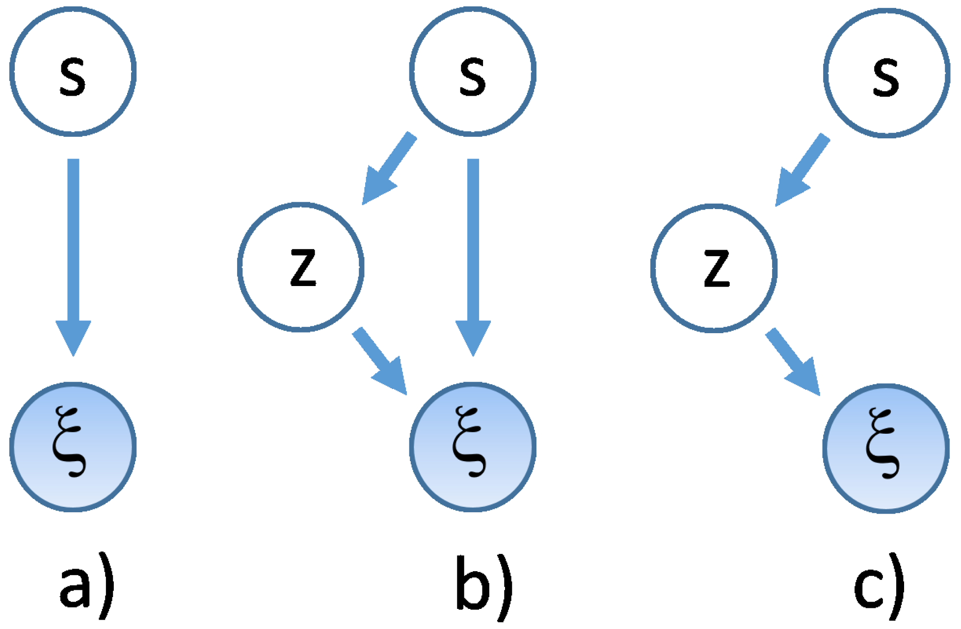
Figure 2.
Alberta power market data: one year from Apr-07-2006 to Apr-06-2007 of hourly data (8760 values). Prices in Canadian Dollars (C$) in the upper panel, and logprices in the lower panel. In this market, during this period, prices are capped at C$ 1000. Notice the frequent presence antispikes, better visible in the logprice panel.
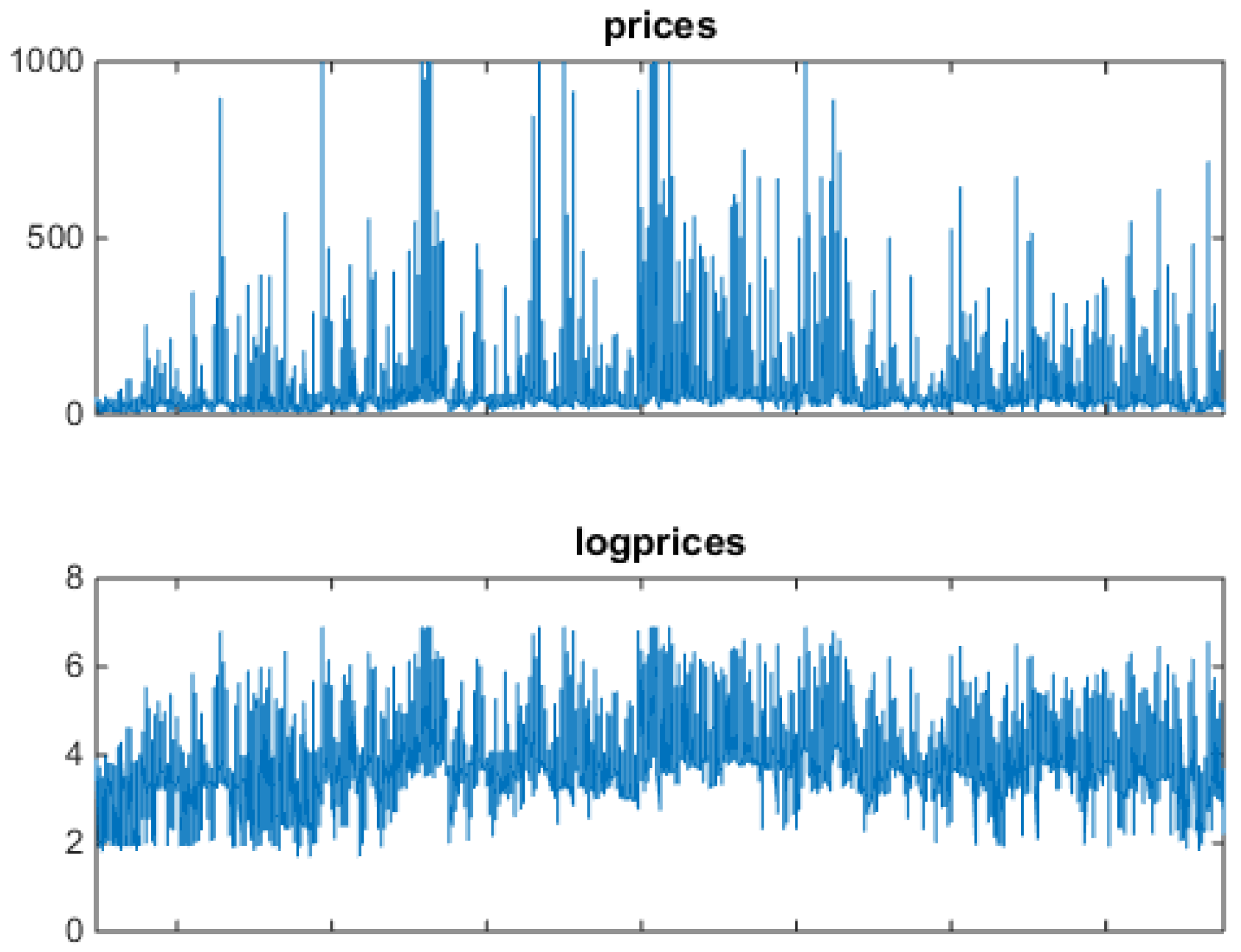
Figure 3.
Alberta power market data blowup: two weeks (336 values) of hourly price and logprice profiles. Prices in the upper panel, and log-prices in the lower panel. Spikes concentrate in central hours, never appear during night time. Antispikes never appear during daylight. On the x axis, progressive hour indexes relative to the data set.
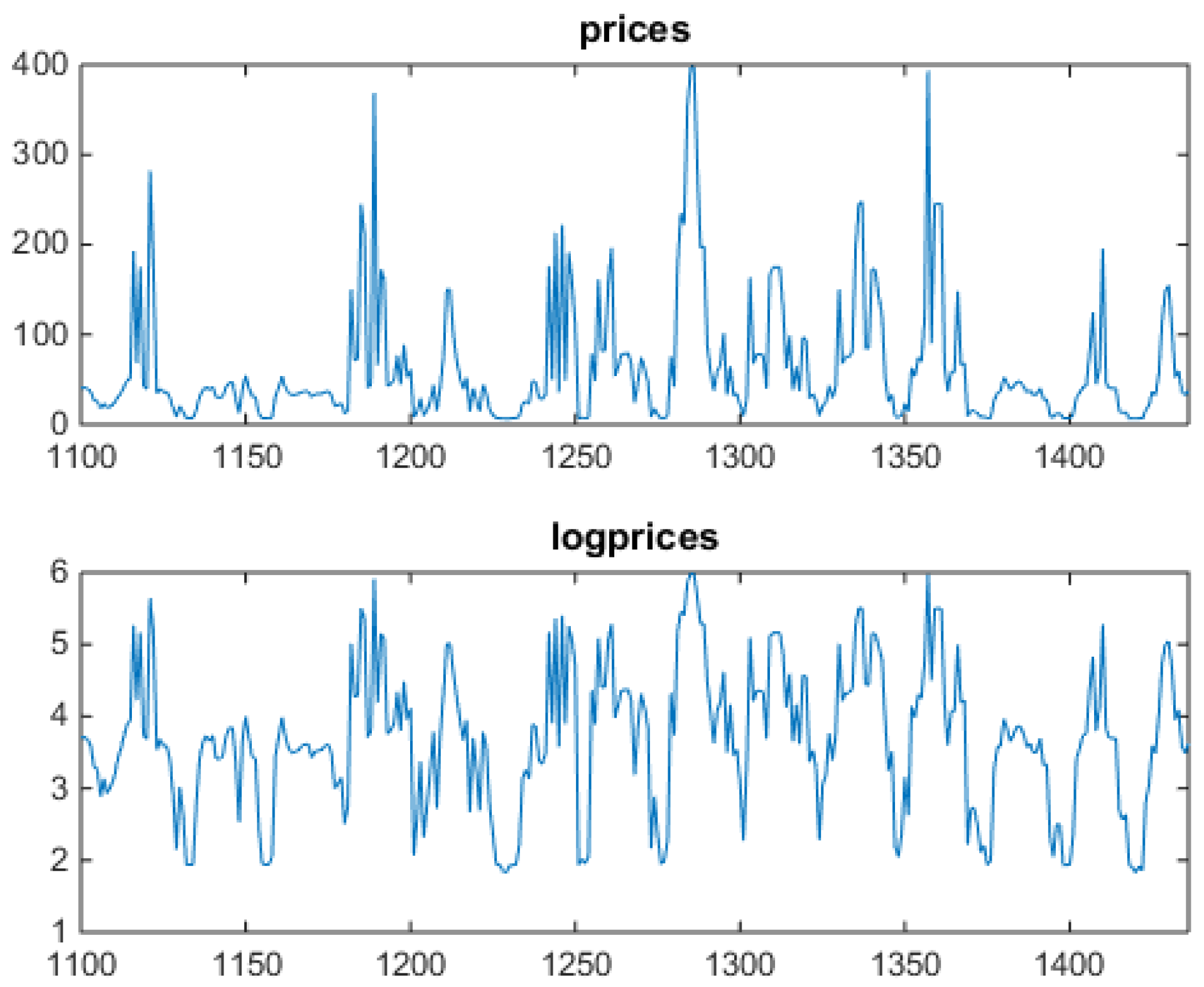
Figure 4.
Alberta power market data: one year from Apr-07-2006 to Apr-06-2007. Upper panel: empirical unconditional distribution of logprices, bar areas sum to 1. Lower panel: autocorrelation of preprocessed timeseries. For each day, at each hour the full data set average of that hour’s logprice was subtracted as .
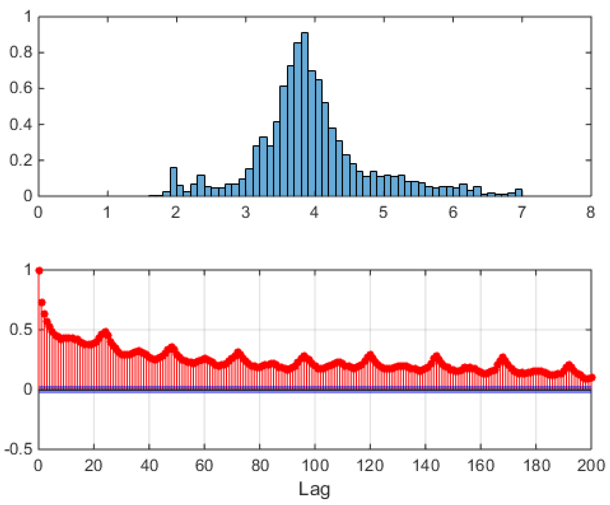
Figure 5.
Four choices of logprice hourly sample distributions (histograms, bar areas sum to 1), and estimated marginals (continuous lines) of a two-component VM. a) hour 1, b) hour 6, c) hour 12, d) hour 18. Notice strong multimodality and skewness in panels b), c) and d).
Figure 5.
Four choices of logprice hourly sample distributions (histograms, bar areas sum to 1), and estimated marginals (continuous lines) of a two-component VM. a) hour 1, b) hour 6, c) hour 12, d) hour 18. Notice strong multimodality and skewness in panels b), c) and d).
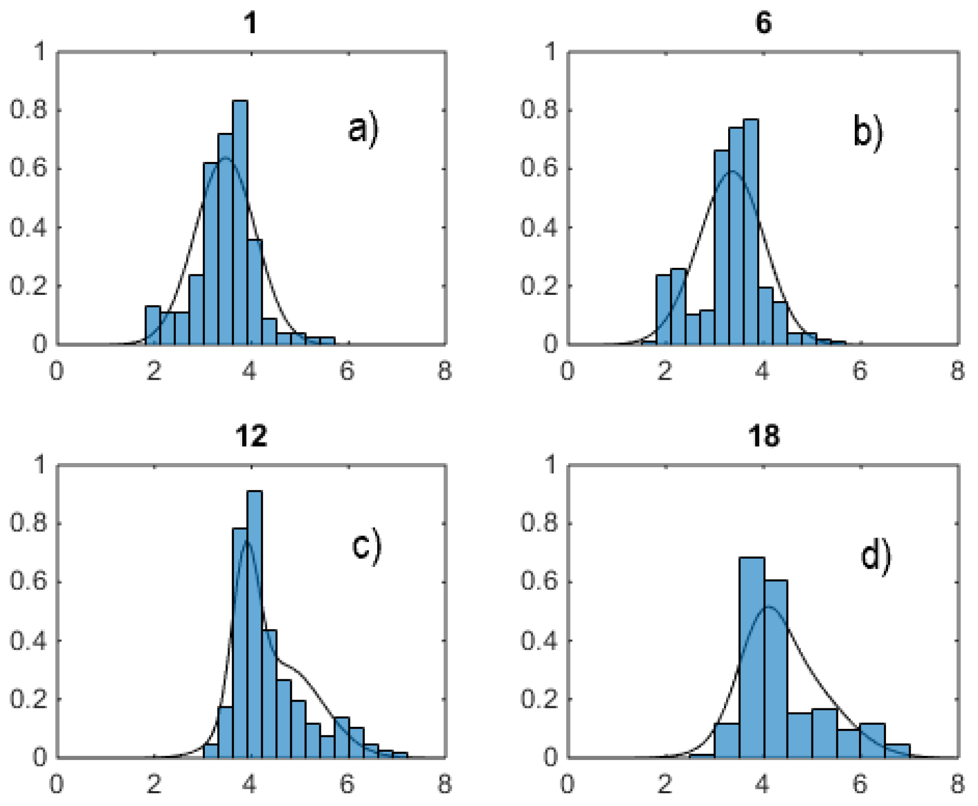
Figure 6.
Hour/hour scatterplots, . 2-dimensional projections of clusters of logprices, hard-clustered with k-means in two clusters, a different model for each panel. Light red (south-west) and dark blue (north-east) distinguish the two populations found. Superimposed black crosses represent cluster centroids. First hour fixed at hour 1, second hour fixed at a) 2, b) 7, c) 13, d) 19. Clusters are not so well separated as with local k-means, but here the algorithm behaves in the same way for all cases.
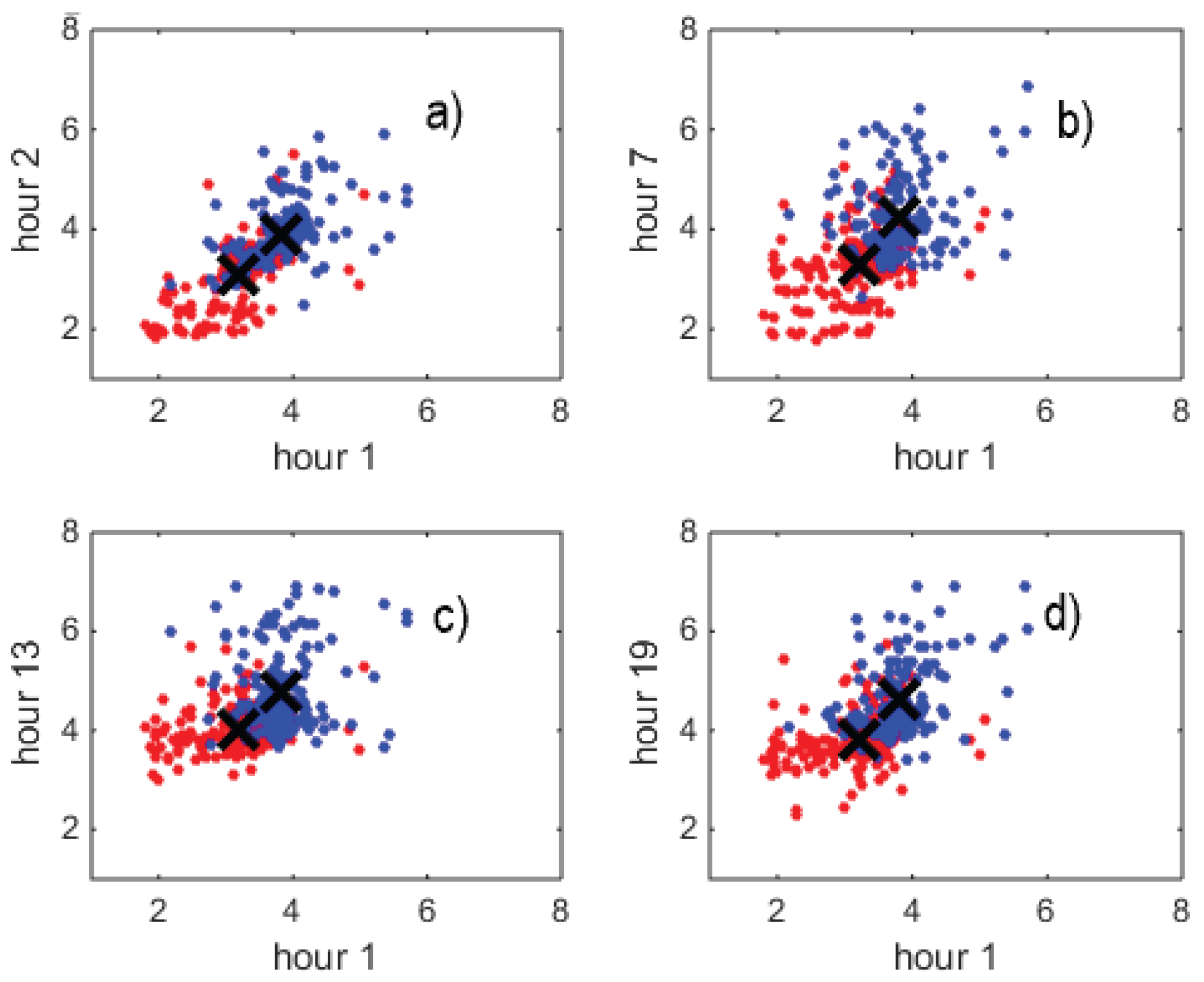
Figure 7.
Two-component VM fit. Sample hourly means (upper panel) and estimated hourly means (lower panel) (solid lines) plus/minus corresponding one standard deviation curves (dotted lines). In the lower panel, is superimposed as a sequence of circles to , to help comparison - they practically coincide. Here BIC=. The number of reruns used to obtain this estimate is 300.
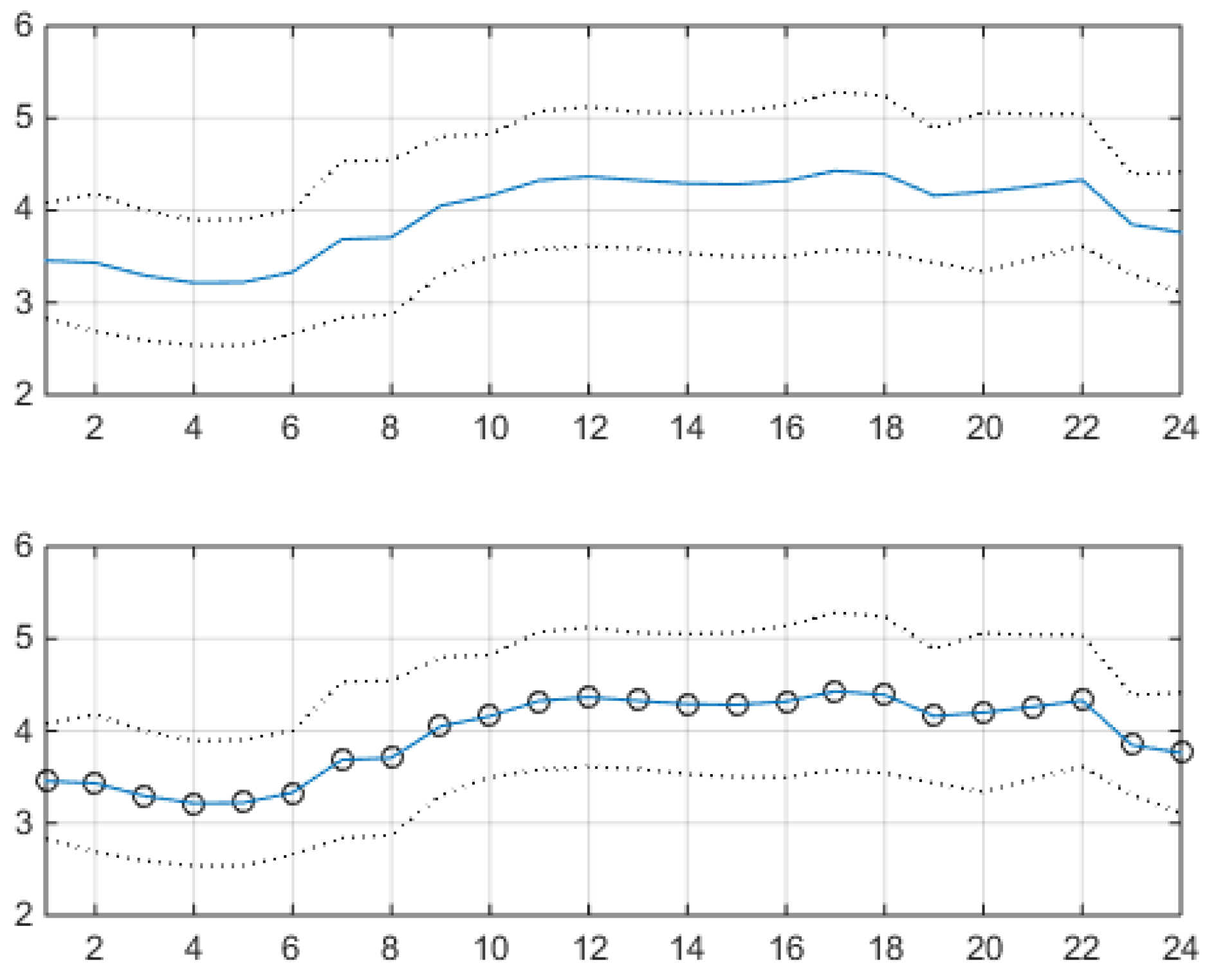
Figure 8.
Two-component VM fit. The upper panel shows the estimated hourly mean of the first component (solid line) plus/minus one standard deviation of the component (dotted lines). The lower panel shows the estimated hourly mean of the second component (solid line) plus/minus one standard deviation of the component (dotted lines). Their weights are and , their weighted sum is in the lower panel of Figure 7.
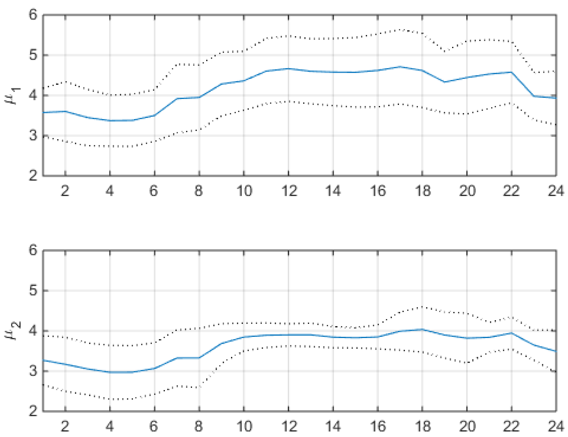
Figure 9.
Two-component VM fit. Estimated hourly component covariances. Upper panel: first component . Lower panel: second component . h on the y- and x-axis. Covariance value scale on the r.h.s..
Figure 9.
Two-component VM fit. Estimated hourly component covariances. Upper panel: first component . Lower panel: second component . h on the y- and x-axis. Covariance value scale on the r.h.s..
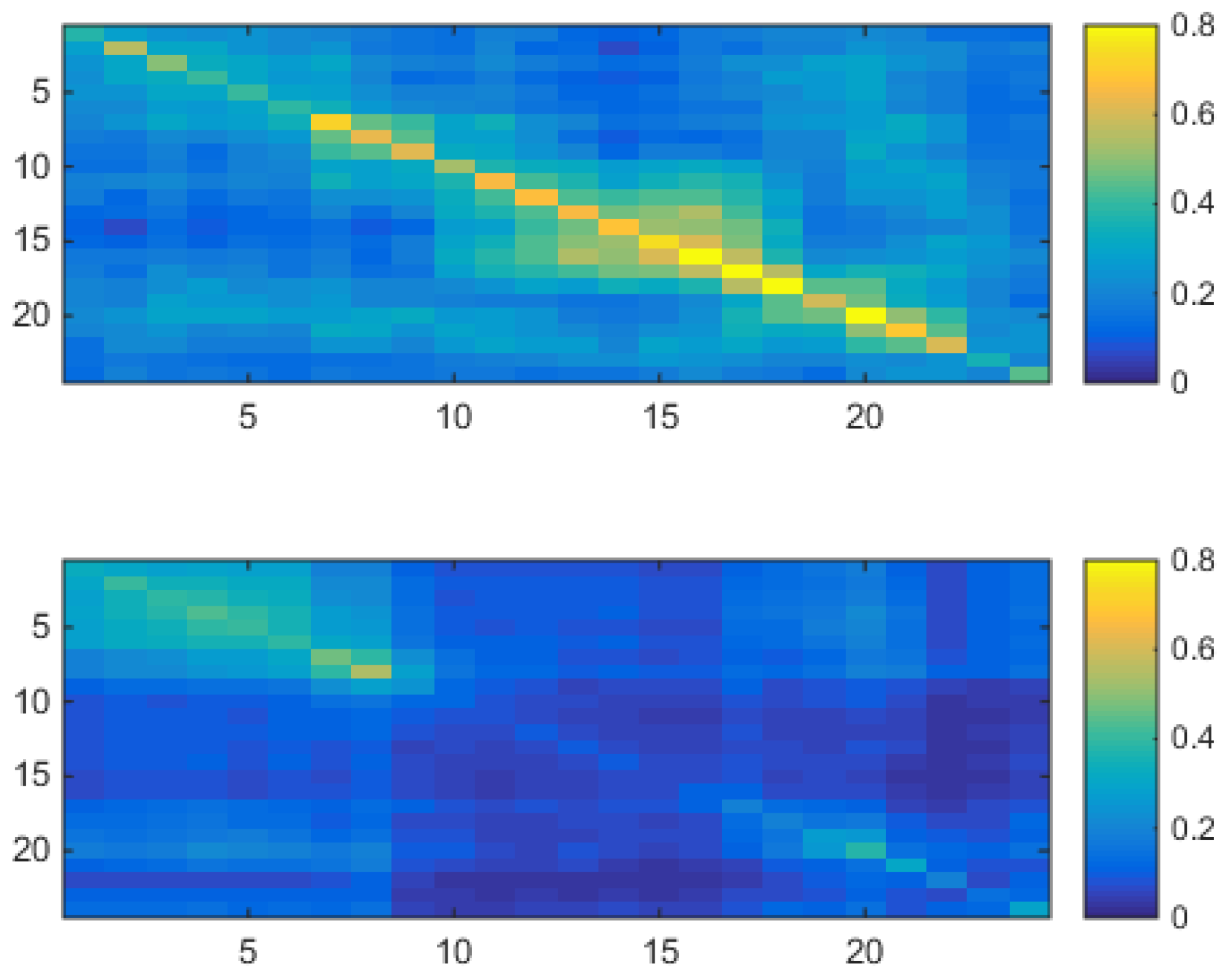
Figure 10.
Two-component VM fit. Mahalanobis distances of individual market days from cluster 1 (upper panel) and cluster 2 (middle panel) centroids. In the lower panel the inferred membership at each day, or , to one of the two clusters. Time scale in days. Large distance from cluster 2 corresponds to large posterior probability of belonging to cluster 1. Market days can be classified ex post in terms of their (hidden) type.
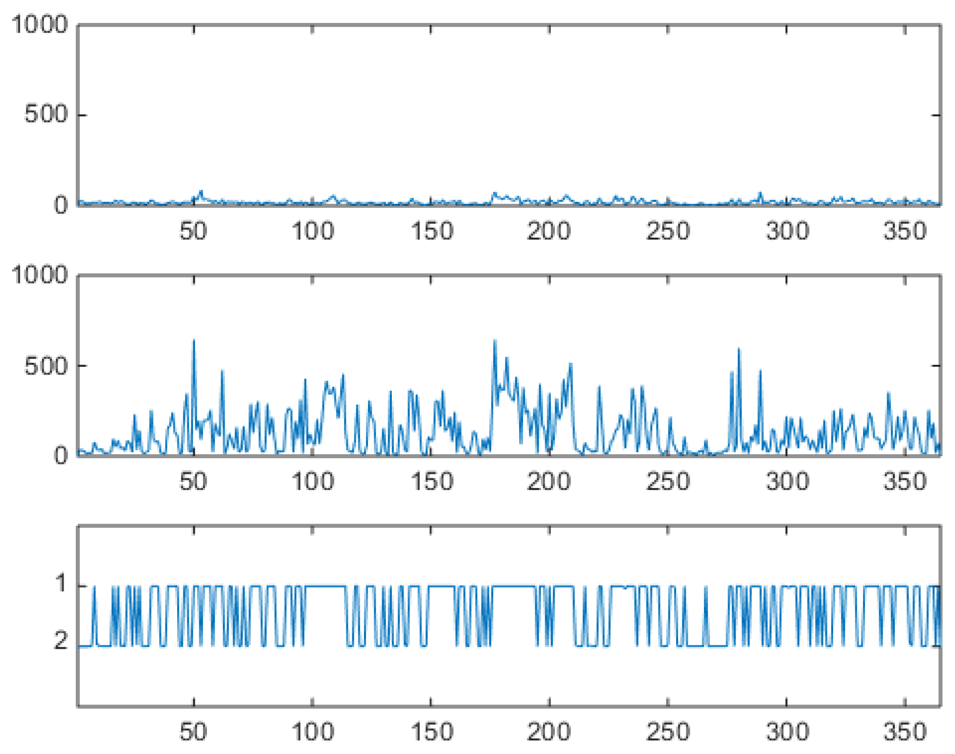
Figure 11.
Fully probabilistic two-component VM fit of a choice of a two-hours marginal (bi-marginal), for the hours 1 and 12. Estimated bi-marginal probability density function, represented in terms of level curves, superimposed to the scatterplot of the market data - i.e., the distribution is seen from above. Data points (i.e., market days 2-d projections) of the scatterplot are marked as light red (south-west) or dark blue (north-east) according to membership inferred from soft clustering. The two peaks of the bimodal 2-d distribution are clearly visible. Compare this soft-clustered scatterplot with k-means hard clustered scatterplots, and their centroid positions. Notice that it is not possible to extract a distribution from k-means.
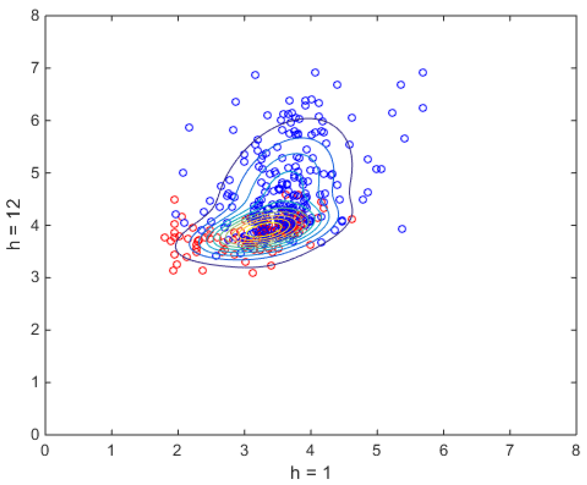
Figure 12.
Synthetically generated series of 365 24-component logprice daily vectors, arranged in one hourly sequence 8760 hours long, sampled from a two-component VM estimated on Alberta data. Upper panel: prices. Lower panel: logprices. On the x axis, progressive hour number. To be compared with the market data series of Figure 2.
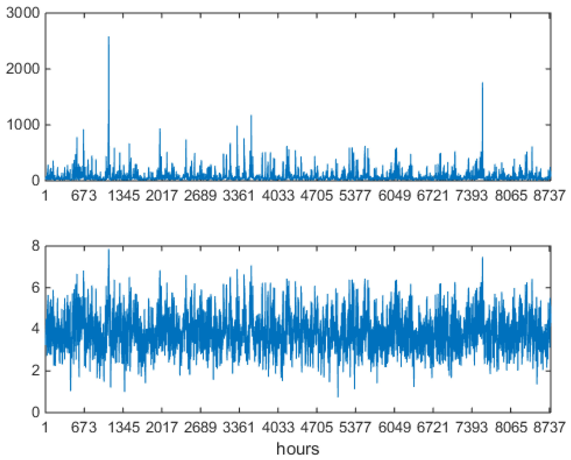
Figure 13.
Blowup of the synthetically generated series of Figure 12, two weeks. Prices (upper panel) and logprices (lower panel). On the x axis, progressive hour number. To be compared with the market data blowup in Figure 3.
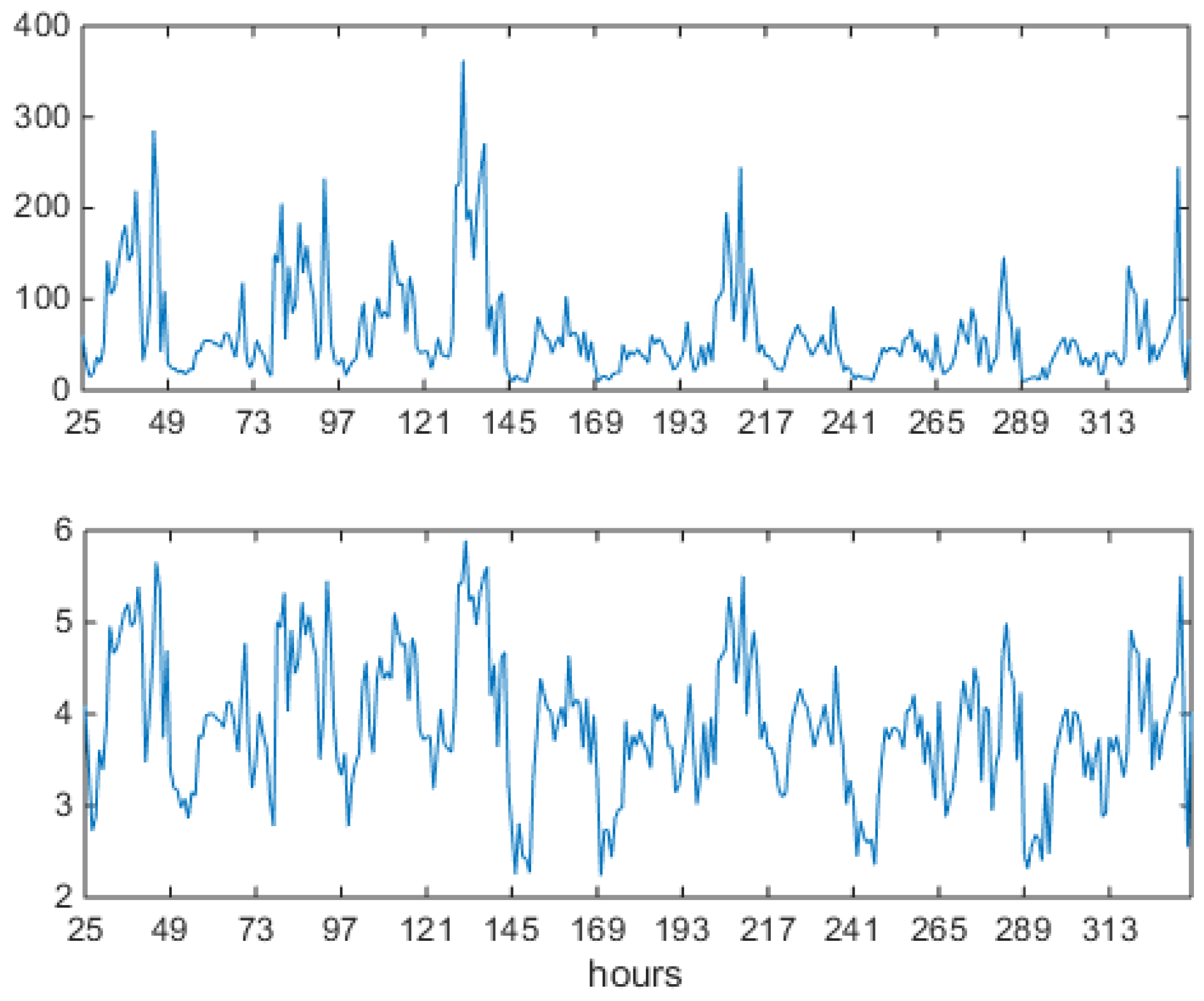
Figure 14.
One year of synthetically generated series of logprices, two-component VM estimated on data. Upper panel: empirical unconditional distribution of logprices, bar areas sum to 1. Lower panel: preprocessed autocorrelation. To be compared with market data autocorrelation in Figure 4. Notice the tail arriving at lag 24 (1 day).
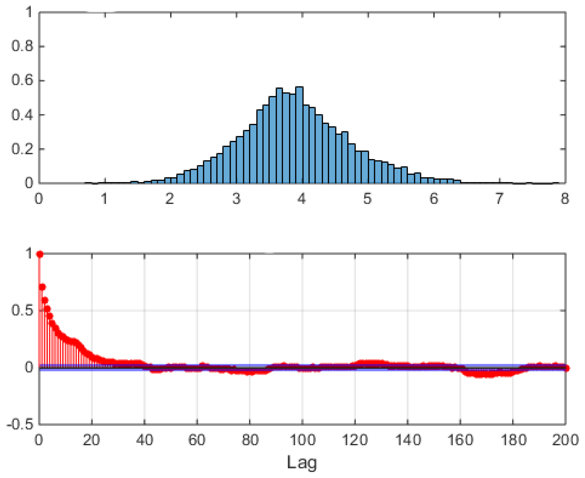
Figure 15.
Types of S-state VHMMs, for , and intermediate layer weight matrices and . a) shallow mixture: one component per state, no intermediate layer; b) untied model, mixtures with components per state that can differ across states, i.e., 6 components in all, associated to for the intermediate layer; c) tied model, mixtures, components in all, associated to for the intermediate layer.
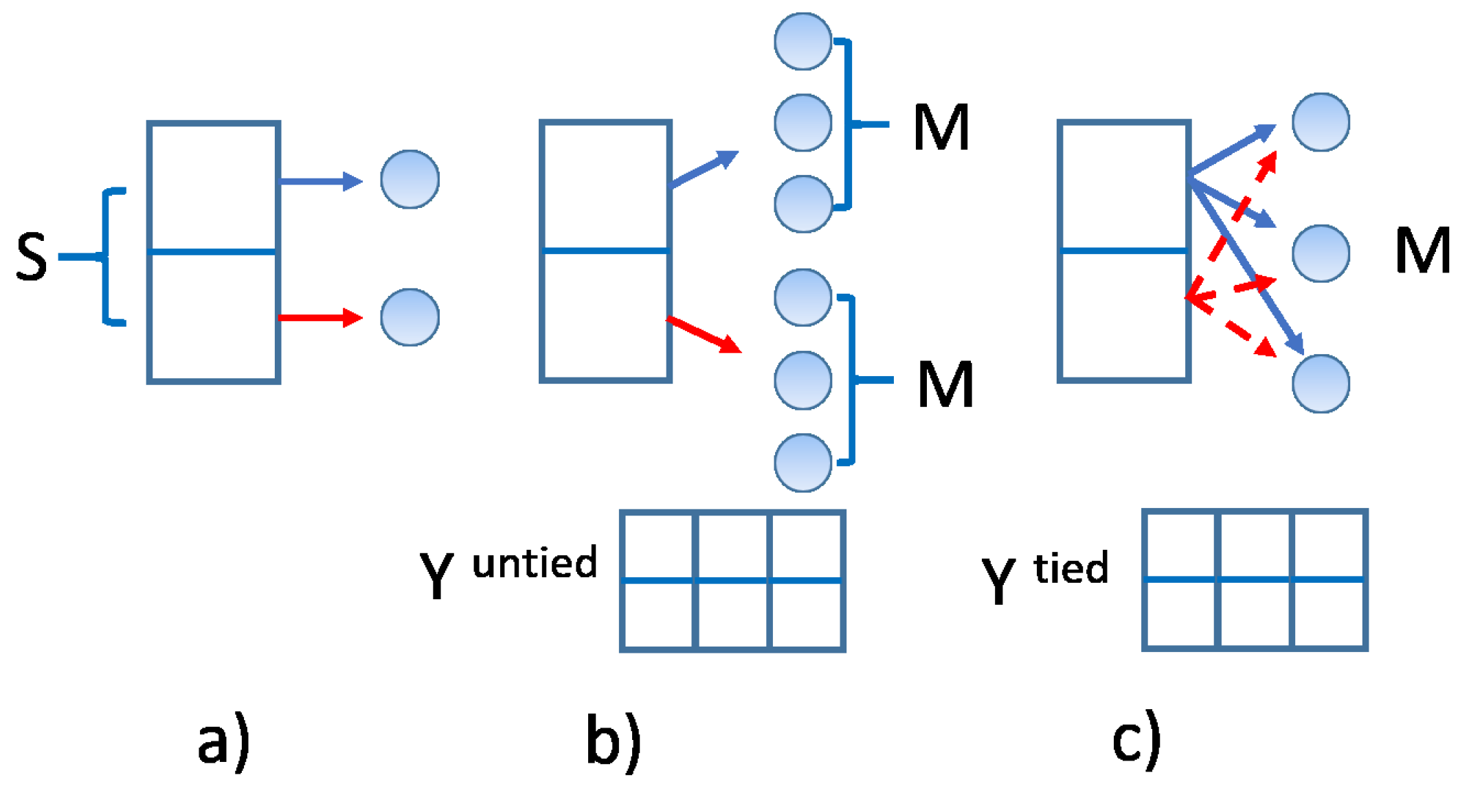
Figure 16.
Two-component tied VHMM fit. Estimated hourly component covariances. Upper panel: first component . Lower panel: second component . h on the y- and x-axis. Compare with the two components of Figure 9 obtained in the shallow VM case.
Figure 16.
Two-component tied VHMM fit. Estimated hourly component covariances. Upper panel: first component . Lower panel: second component . h on the y- and x-axis. Compare with the two components of Figure 9 obtained in the shallow VM case.
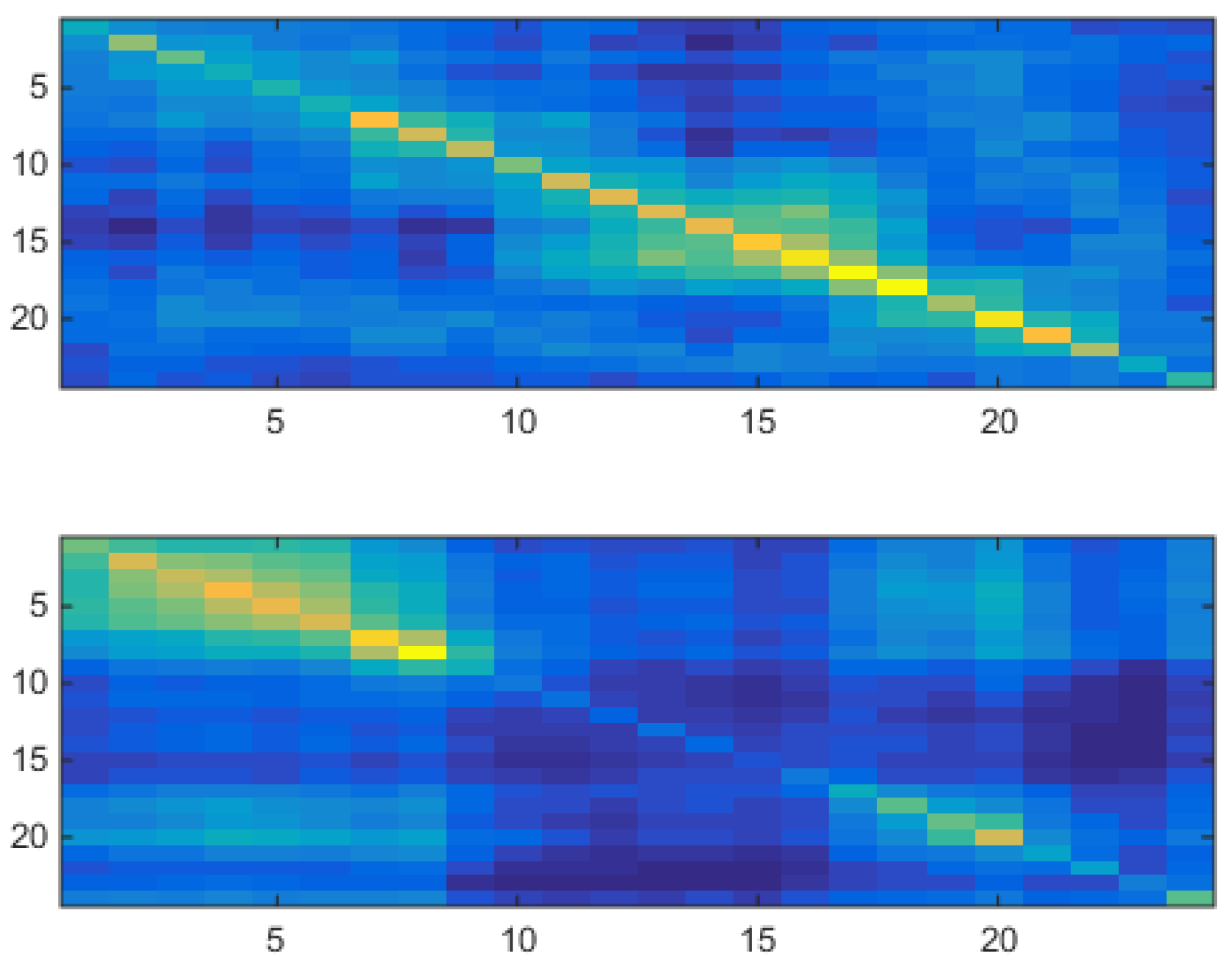
Figure 17.
Two-component tied VHMM estimated yearly on logprice data. Synthetically generated series for prices, logprices and hidden states. Upper panel: prices. Middle panel: logprices. Hours on x-axis for upper and middle panels. Lower panel: state trajectory . Days on x-axis for the lower panel. State membership controls spikiness: for spikiness is higher than for . Compare with component covariances of Figure 16.
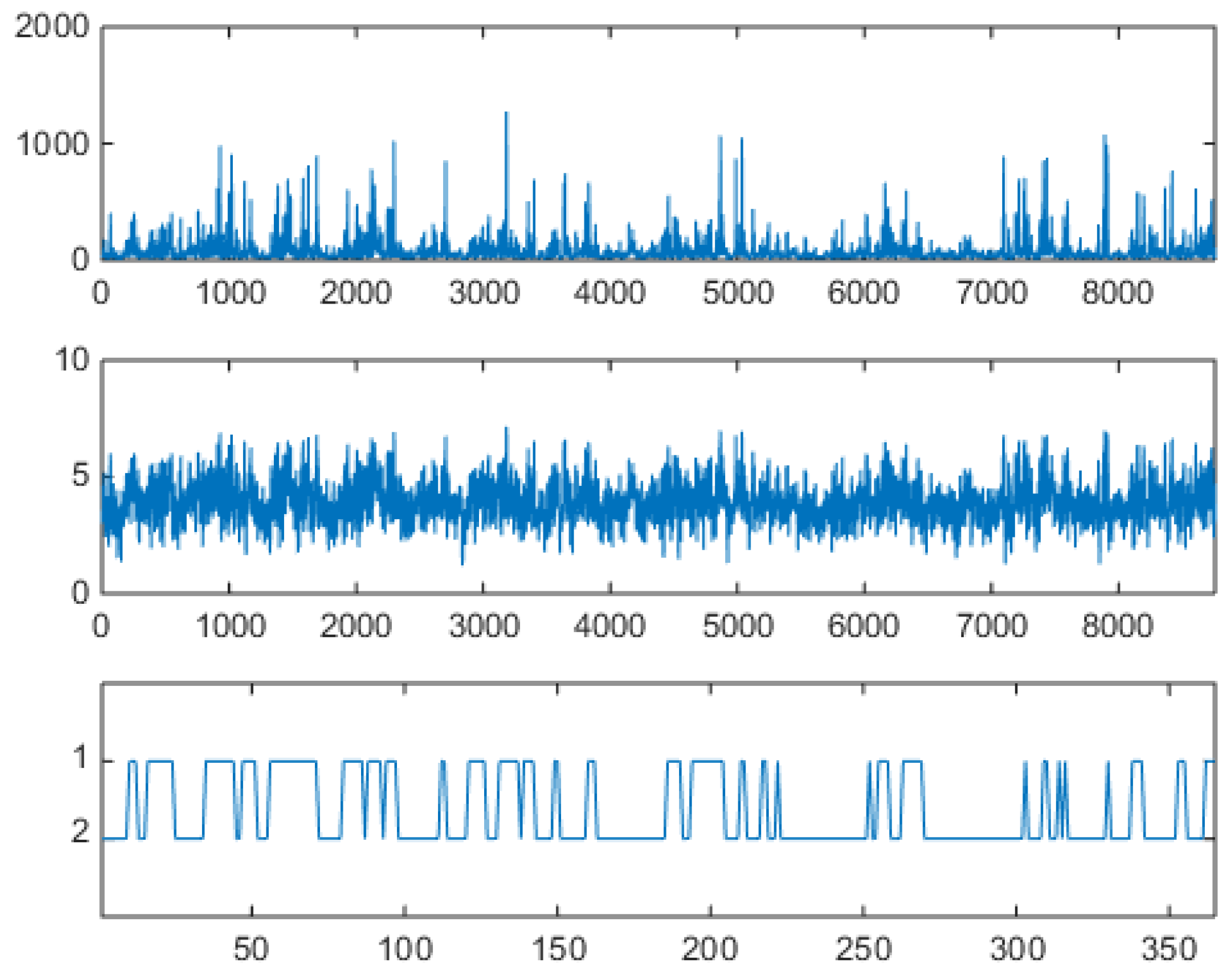
Figure 18.
Two weeks of synthetically generated series of prices (upper panel) and logprices (lower panel), one full year estimate, two-component tied VHMM estimated on logprice data. Hours on the x-axis for both panels. To be compared with market data series of Figure 3.
Figure 18.
Two weeks of synthetically generated series of prices (upper panel) and logprices (lower panel), one full year estimate, two-component tied VHMM estimated on logprice data. Hours on the x-axis for both panels. To be compared with market data series of Figure 3.
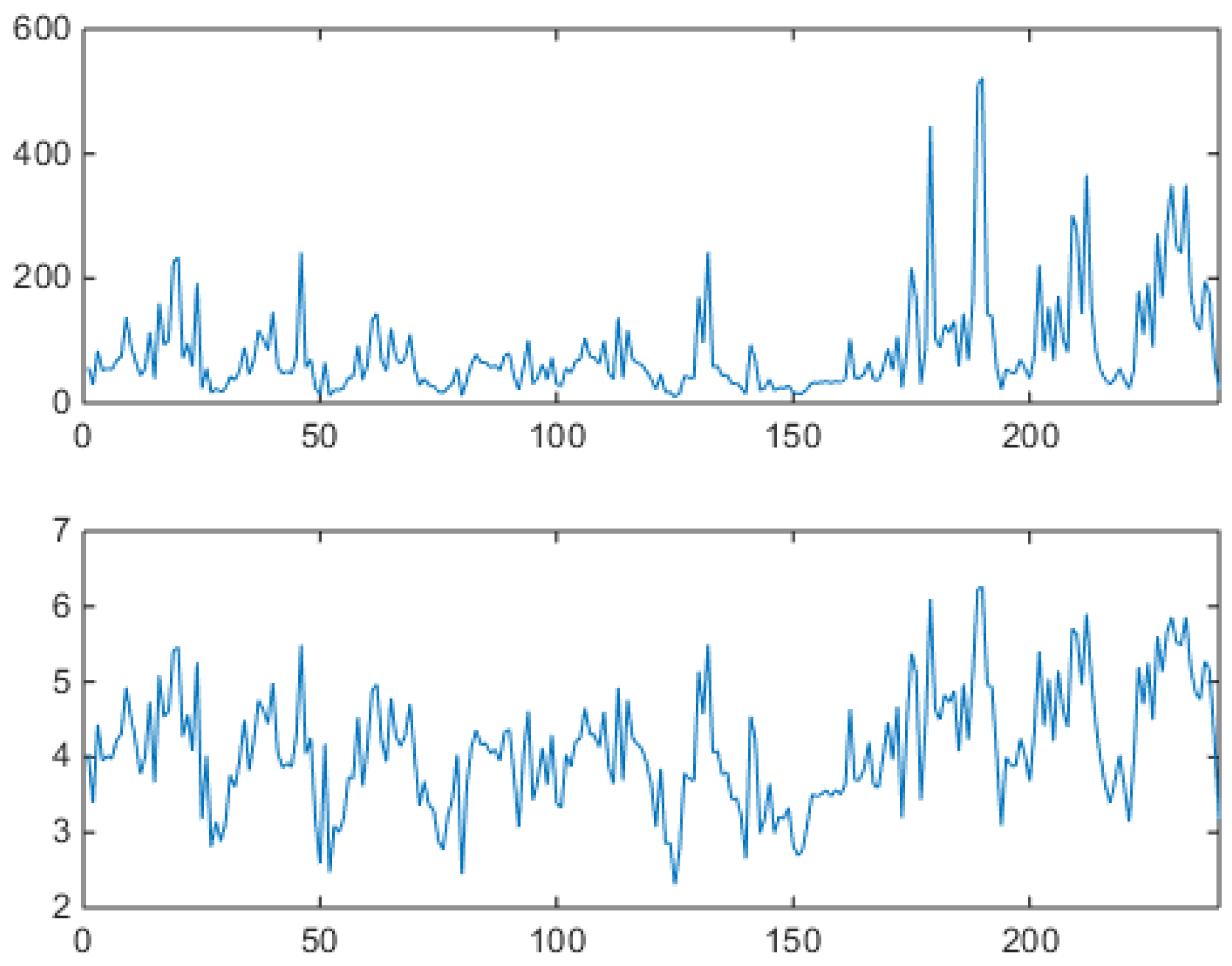
Figure 19.
One year of synthetically generated series of logprices, two-component tied VHMM estimated on one year of logprice data. Upper panel: empirical unconditional distribution of logprices, bar areas sum to 1, logprices on the x-axis. Lower panel: preprocessed autocorrelation. Notice the tail arriving at lag 48 (2 days). To be compared with the autocorrelation of original market data series of Figure 4 and to the VM autocorrelation of Figure 14, which arrives at lag 24.
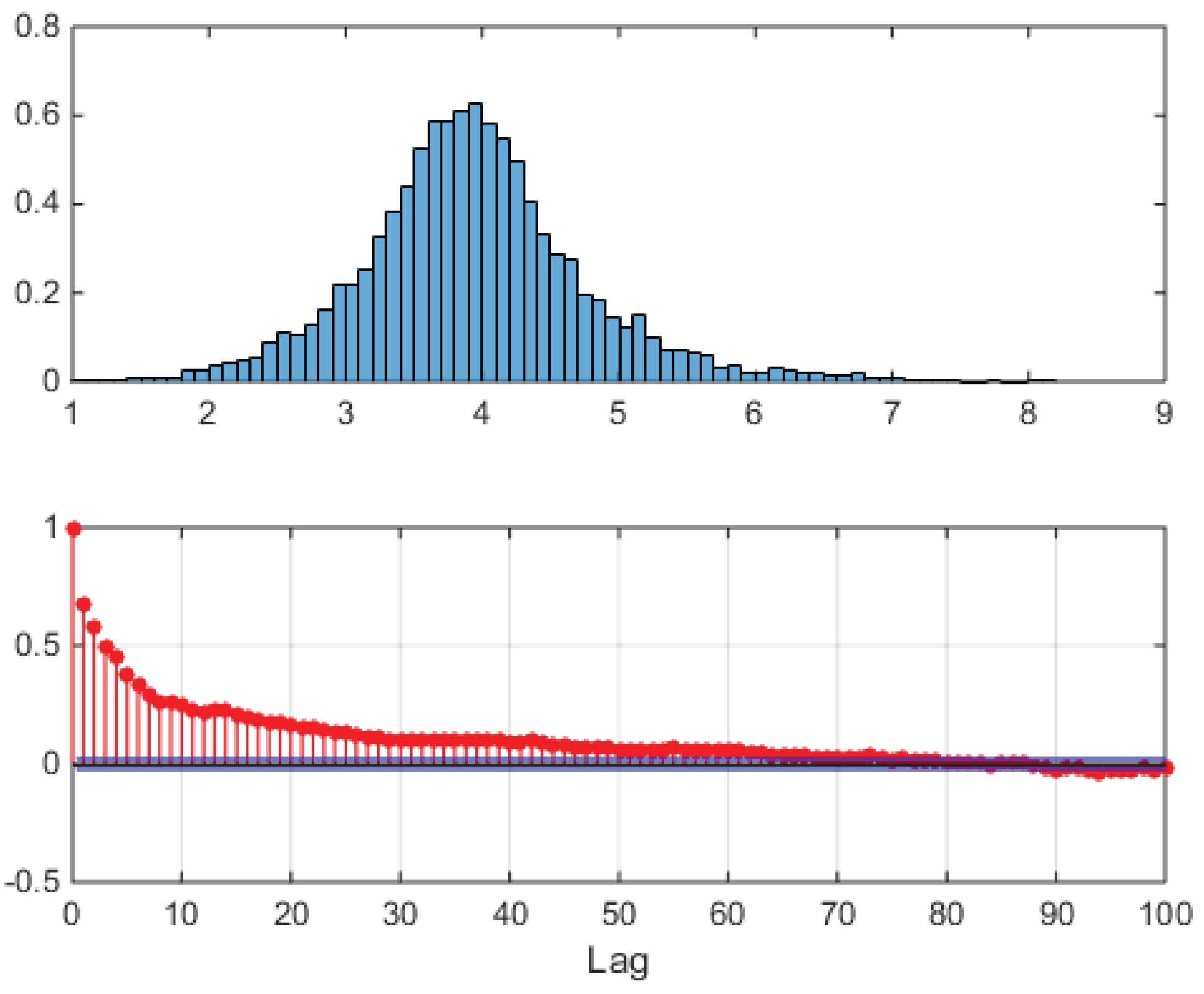
Figure 20.
Sample autocorrelation functions of three synthetically generated samples from a two-component tied VHMM estimated yearly on logprice data. Upper, middle and lower panels: sample autocorrelations. Lag scale on the x-axis extends to four days. These profiles are rather different. Notice the short autocorrelation in the lower panel.
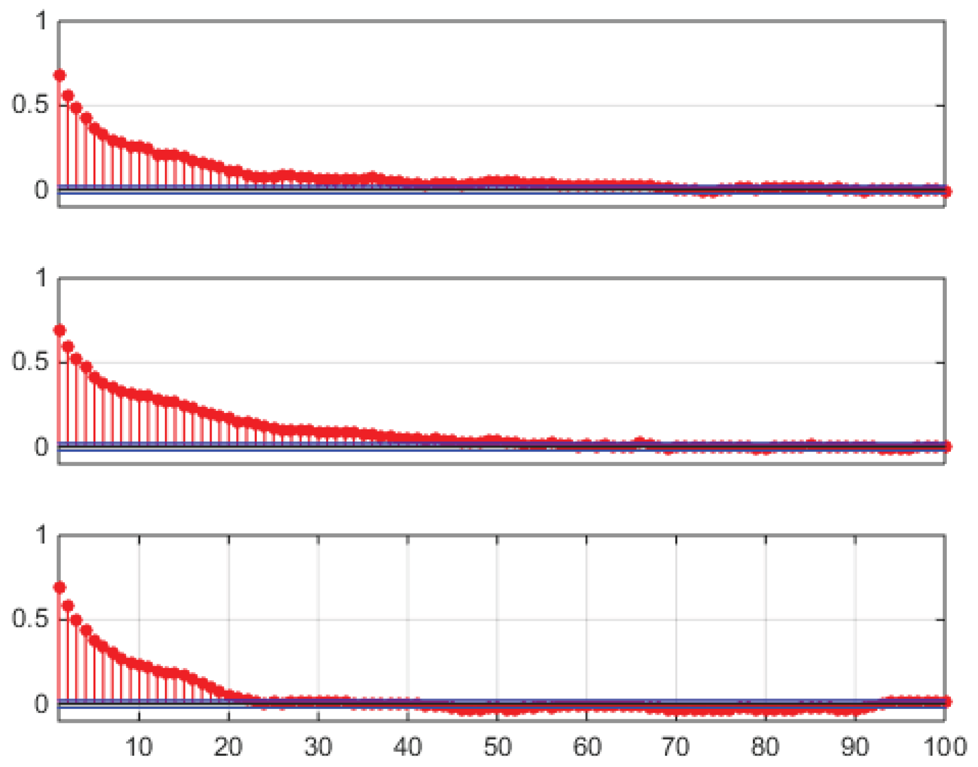
Disclaimer/Publisher’s Note: The statements, opinions and data contained in all publications are solely those of the individual author(s) and contributor(s) and not of MDPI and/or the editor(s). MDPI and/or the editor(s) disclaim responsibility for any injury to people or property resulting from any ideas, methods, instructions or products referred to in the content. |
© 2025 by the authors. Licensee MDPI, Basel, Switzerland. This article is an open access article distributed under the terms and conditions of the Creative Commons Attribution (CC BY) license (http://creativecommons.org/licenses/by/4.0/).
Copyright: This open access article is published under a Creative Commons CC BY 4.0 license, which permit the free download, distribution, and reuse, provided that the author and preprint are cited in any reuse.


