
Submitted:
16 July 2025
Posted:
17 July 2025
You are already at the latest version
Abstract
The global shift to sustainable energy has led to a significant growth in the penetration of renewable energy sources (RES), mainly wind and solar electricity, in electrical grids. Although these resources offer substantial environmental and economic benefits, their incorporation presents challenges stemming from unpredictability, intermittency, and limited controllability. This article addresses the challenges associated with high penetration of renewable energy into the grid, including the management of power output uncertainty using quasi-dynamic simulation tools for both short- and long-term periods, as well as the analysis of profits, losses, and energy of a wind farm utilizing both basic energy analysis and probabilistic analysis in conjunction with Monte Carlo Simulation (MCS). This study is essential to ensure that the grid remains secure against stability challenges arising from fluctuations in power production from renewable energy sources.
Keywords:
decentralized energy systems
; photovoltaic (PV) plant
; uncertainty of renewable energy (RE)
; Wind farm
; demand response
1. Introduction
Traditional power networks are characterized by a limited number of centrally situated, high-capacity plants. Many countries are undergoing a swift transition to RE generation [1]. The global energy industry is experiencing a profound revolution propelled by the imperative to address climate change, decrease greenhouse gas emissions, and shift towards sustainable energy sources [2]. One of the primary measures is the enhanced incorporation of RES—specifically wind, solar, and hydropower—into electrical power systems [3]. This transition, also known as the high penetration of RE, has accelerated due to technical innovations, favourable regulations, and decreasing costs of renewable technologies [4]. This transformation offers significant environmental and economic advantages, although it also presents several technological and operational hurdles for grid operators. In contrast to traditional fossil fuel-based generation, renewable energy sources are intrinsically changeable, reliant on meteorological conditions, and regionally distributed [5].These attributes can affect grid stability, reliability, and efficiency if inadequately handled [6].
The research reveals that energy efficiency and RE technologies are fundamental components of the shift, and their synergies are equally significant [4]. RE has the potential to fulfill two-thirds of world energy demand and significantly aid in the reduction of greenhouse gas emissions required to maintain the average global surface temperature increase below 2 °C by 2050 [7]. A growing array of indications suggests a rapid energy transition that may significantly impact energy supply and demand in the forthcoming decades [8].
The shift towards substantial RE integration in power systems is propelled by a confluence of environmental, economic, technical, and policy-related influences [9]. These factors are reshaping the global energy framework and expediting the incorporation of RES such as solar, wind, and hydropower into electrical networks [2]. Presented below is a systematic summary of these major factors in Table 1.
This research examines the KK II Solar PV Plant, which is presumably one of the RE initiatives established under South Africa’s Renewable Energy Independent Power Producer Procurement Programme (REIPPPP) [15]. KK II solar PV is in the Northern Cape, South Africa (many RE projects are situated there due to high solar irradiance). This PV plant has a total installed capacity of 75MW [16]. Secondly, this study uses Metro Wind Van Stadens Wind Farm situated in the Eastern Cape, with an installed capacity of 27 MW, including 9 turbines of 3 MW each [17]. Figure 1(a & b) elegantly illustrates a solar power plant at sunrise, representing the emergence of renewable energy options. Figure 1 (c & d) illustrates the operation of wind energy, wherein these turbines transform kinetic wind energy into electricity, therefore enhancing a cleaner power system.
2. Background Overview
The incorporation of a substantial amount of RE into the power grid signifies a dramatic change in global energy systems [2]. The shift to high penetration of RE in power networks is essential for worldwide initiatives aimed at decarbonizing the energy sector, improving energy security, and fostering sustainability [18]. High-penetration of RE is a scenario in which a substantial percentage—generally 30% or greater—of a grid’s electrical output is derived from renewable sources, including solar, wind, hydropower, and biofuels [19].
2.1. Renewable Grid in South Africa
Renewable Grid Firming in South Africa encompasses a collection of tactics and technology implemented to provide a reliable and stable electrical grid while accommodating the growing integration of variable renewable energy (VRE), including wind and solar sources [20]. As South Africa transitions from a coal-centric energy framework to a cleaner, more sustainable model, grid firming is important owing to the sporadic nature of RES [21]. Figure 2 represents the anticipated power generation composition for South Africa, contrasting data from 2010 with forecasts for 2050 [22].
The long-term approach targets a net-zero power mix by 2050, incorporating wind, solar, hydro, biomass, and maybe nuclear energy [23]. Despite the reliance on fossil fuels, RE has also been on an upward trend, with wind energy contributing significantly [24].
Table 2 indicates that coal continues to be the primary source of power in South Africa due to the country’s large coal reserves; nevertheless, the promotion of RE is essential and cannot be overlooked until coal is exhausted and attention shifts to RES.
2.2. Load Demand Uncertainty
Uncertainty in Load Demand pertains to the unpredictability and variability linked to future power consumption trends [25]. This unpredictability presents difficulties for power system design, operation, and dependability, particularly for the integration of RES and advanced smart grid technology [26]. The concerns associated with RE that must be considered when integrating it into the system are illustrated in Table 3.
Several variables contribute to load demand uncertainties, including weather variations, in which temperature, humidity, and cloud cover have a substantial impact on energy use, notably for heating and cooling [30]. Economic fluctuations, which are Industrial and commercial demand, can be challenging to anticipate [31]. There are two categories of uncertainty in loads: Short-Term Uncertainty, which encompasses variations in demand that occur minutes to days in advance (e.g., weather-induced fluctuations). Long-Term Uncertainty, which encompasses months to years in advance (e.g., demographic shifts, policy changes) [32].
2.3. Grid Reliability
As the proportion of RE in a power system increases substantially, maintaining grid resilience becomes more intricate. This is attributable to the fluctuating and unpredictable characteristics of resources such as solar and wind energy [1]. It is crucial to accurately capture significant transient dynamics that may lead to network failure in actual power grids, as well as the emerging power-balancing and stabilizing characteristics of these interconnected systems [33]. Prediction Uncertainty stemming from erroneous forecasts of renewable energy generation impacts system stabilization and reserve planning [34]. Flexible generation, such as gas turbines or hydroelectric facilities, enables rapid adjustment to mitigate the unpredictability of renewable energy [35].
3. Design and Implementation of RE into the Grid
This section illustrates the integration of RE into the grid, outlining the mathematical methodologies employed in the construction of both wind farms and solar PV plants, aimed at diminishing the reliance on fossil fuels, which adversely impact both the environment and human health.
3.1. Uncertainty of Wind Power
Wind Energy Uncertainty signifies the unpredictable nature of wind energy generation resulting from the variability and limited controllability of wind resources. Unpredictability poses significant challenges for power system design, operation, and reliability, especially with the increasing integration of wind generation. The wind speed follows a Weibull distribution, with the probability density function (PDF) utilized for the wind variations.
The scaling index c may be derived from the average wind speed at a certain location, as seen in
Take into account the wind velocity, shape factor, and scale factor, referred to as, and, respectively, where, and Then, the wind power output can be stated as
, and are recognized as cut-in wind speed, rated wind speed, and cut-out wind speed, respectively. is the rated power of a wind unit.
The probability of each condition is expressed by the following equation:
Whereby
Where and represent the velocity restrictions in state w.
3.2. Unpredictability in Decentralized Solar Energy
The swift implementation of localized solar energy systems has revolutionized power generation by fostering sustainability and energy autonomy. The intrinsic unpredictability of solar energy generation presents considerable hurdles to grid stability, energy planning, and storage management [36]. Weather unpredictability, seasonal fluctuations, and the geographic distribution of PV systems contribute to inconsistent energy production, complicating precise forecasting [37]. The absence of centralized coordination among several small-scale producers complicates demand-supply equilibrium and grid integration.
The stochastic lighting intensity is the predominant component in solar generation. Numerous studies have shown that the probability density function adheres to the Beta distribution as
Wherebystands for Gamma function, andare the considerations,is the illumination intensity,is the maximum value. The communication between the illumination intensity and the output power of a solar unit can be described as
Whererepresents the rated value and represents the rated output power of the solar unit.
This study used quasi-dynamic simulation, a modeling method that lies between steady-state and fully dynamic simulations. It illustrates the evolving behavior of a system over time in a simplified, often discontinuous or stepwise manner, rather than continuously recreating every transient characteristic. This method is utilized when extensive dynamic simulations are too resource-demanding or unnecessary, yet steady-state analysis does not sufficiently capture important time-dependent processes
3.3. Available Transfer Capability (ATC) on the Wind Farm
Available Transfer Capability (ATC) indicates the highest supplementary power transfer capacity in the transmission network that may be utilized without breaching system restrictions (including temperature, voltage, and stability constraints) after considering existing commitments. In the context of wind farms, ATC pertains to the extent of supplementary wind-generated electricity that can be integrated into the grid and supplied to load centers. This network utilizes the boundary to ascertain the available transfer capability of the wind farm, excluding the rest of the network, to evaluate losses, earnings, and energy output of the wind farm.
The total transfer capability (TTC) is less than the transmission reliability margin (TRM), which is lower than the capacity benefit margin (CBM), and is also smaller than the aggregate of existing transmission commitments (ETC). This research did not examine TRM or CBM. Consequently, the ATC may be calculated by deducting the TTC from the ETC.
ATC = TTC − ETC
Whereby
Subjected to
Where B is the set of all buses,is the active power at the generator I, andis the active power demand at the bus , is the voltage phase angle between the busand is the scalar parameter.
This approach is intended for computing the ATC utilizing Monte Carlo simulations with a sensitivity analysis.
3.4. Design of the Wind Farm and PV Plant
This section discusses the implementation of both the wind farm and solar photovoltaic plant within DIgSILENT PowerFactory software. It outlines the design of wind turbines by including wind speed, the wind power curve, wind power capacity, distribution, and correlation. Furthermore, it indicates the design of the solar PV plant and its load characteristics, offering detailed information on the solar PV plant before its integration into the grid.
Figure 4 illustrates the KK II solar PV plant, with 15 solar PV units, each producing 5 MW, with an apparent power of 7 MVA and a power factor of 0.9, utilizing active power input for energy generation. The solar PV systems are interconnected by an 11kV busbar and a 1km cable. Additionally, a 100MVA step-up transformer with a voltage rating of 11/22kV is employed to elevate the voltage to 22kV in KK II Solar PV, as seen in Figure 4. Figure 3 illustrates the voltage levels more effectively, with a minimum voltage of 16.5kV and a maximum voltage of 345kV.
Figure 5 shows the wind farm integrated into the 39 bus England System, with 11 wind turbines, each rated at 2.778 MVA with a power factor of 0.9. The wind turbines are interconnected via an 11kV busbar and a 1km cable.
Figure 6 illustrates the wind power curve applicable to all wind turbines utilized in this study; it is evident from this curve that the turbines achieve maximum power production at a wind speed of 16 m/s.
The wind power capability curve describes the operational limits of an electrical generator, specifying the restrictions on the active and reactive power it can produce. The circle defines the boundary of all operational locations as seen in Figure 7.
The subsequent characteristics of wind turbines dictate the quantity of wind generated, fluctuating bi-hourly throughout the year. Winds 1 and 8 exhibit identical temporal features as seen in Figure 8, as do winds 3,9 and 10 as shown in (b).
The periodic characteristics of the KK II solar PV Plant exhibit bi-hourly fluctuations throughout the year, resulting in considerable unpredictability in the generated output power, as seen in Figure 9
Figure 10 describes the characteristics assigned to both sources. Figure 10(a) shows the transformed distribution assigned to the wind turbine, incorporating wind speed and the Weibull curve. Figure 10 (b) depicts the allocation of prediction errors among generators and solar PV systems to forecast possible future mistakes. Figure 10(c) illustrates the utilization of the Weibull distribution for wind speed, employing the shape and scale parameters provided in Table 4.
Figure 10(d) illustrates the correlation distribution utilized to establish a relationship among the 11 wind turbines in the wind farm, with the correlation coefficient established at 0.99. A higher coefficient indicates a stronger relationship, with a value of 1 representing a perfect correlation.
4. Results
The case study is carried out and modeled in DIgSILENT PowerFactory, employing a wind farm located in the Northern Cape of South Africa, with an installed capacity of 75 MW. The 15 solar PV units, each having a capacity of 5 MW, are employed to produce energy from the KK II solar PV facility for the grid. It emphasizes the imperative of upgrading transmission lines to meet future demand while incorporating renewable energy into the current system, so improving electricity accessibility while accounting for the inherent power unpredictability of these sources. The findings are derived from load flow analysis employing the Newton-Raphson approach, while short- and long-term planning is executed via quasi-dynamic simulation to predict the potential available power across different periods. This method also enables the identification of whether the grid functions within allowable parameters, thereby reducing equipment overload and ensuring busbar values stay within acceptable levels to avoid grid instability.
Figure 11 illustrates the simulated Metro wind farm, of 11 identical wind turbines, each generating 2.5 MW, which corresponds to 90% of their maximum capacity at a wind speed of 16 m/s. The total power generated is 27.39 MW, with minimal losses in the cables. This network indicates that the facility operates under typical conditions, as evidenced by the little box. Healthy components of the grid are represented by green in the little box in Figure 11, whereas the unhealthy components are shown by blue or red, depending on whether the voltage is low or high.
Figure 12 represents the KK II solar PV plant, with 15 identical solar PV units, each generating 5 MW, or 71.4% of their total capacity. The total power output is 73.26 MW, with 1.74 MW lost in the cabling connecting the busbars. The KK II solar PV power system operates within acceptable parameters, hence improving system stability.
Figure 13 illustrates the p.u. voltage over one year for the busbar in the wind farm. Despite variations, all busbars within the network function within constrained limitations.
Figure 14 illustrates the metro wind farm undergoing quasi-dynamic simulation. Each wind turbine has distinct characteristics, as seen in Figure 8, resulting in variations every thirty minutes throughout the year. It demonstrates that WT1 has differing active power levels relative to WT3
Figure 15 illustrates the solar power plant under quasi-dynamic simulation, containing 15 solar PV units with distinct characteristics, as previously detailed in Figure 8. The figure demonstrates that PV1 differs from PV2 and PV3, highlighting the inherent uncertainty associated with RE. Furthermore, in contrast to Figure 12, the PV plant is currently generating a total output of 59.16 MW
The variability in loading, evidenced by the non-uniform shape, contrasts with Figure 13, suggesting an anomaly in the voltage at busbar K in Figure 16. It illustrates that the PV plant functioned for one year, with the graph’s fluctuations indicating electricity production variations over different seasons, including vacations and weekends.
Figure 17 illustrates the busbar voltage p.u., indicating that all busbar voltages remain within permissible limits. Additionally, it is observed that the voltage decreases as load demand escalates.
Figure 18 displays the line voltage in p.u, which is still within permissible limits despite having increased in comparison to Figure 17. Moreover, Figure 18. illustrates that the PV plant operated for a decade, from 2024 to 2034. As the load demand escalated, the voltages on the busbars dropped, although they remained within permissible limits.
In conclusion, it is essential to emphasize RE to mitigate the use of dwindling fossil fuels. This study demonstrates how to analyze the PV plant to guarantee that its connection to the grid does not threaten grid stability.
The energy study of the wind farm is executed utilizing a fundamental calculation method, which carries out a sequence of load flow computations over the spectrum of wind speeds from zero to the highest speed being evaluated. The wind farm consists of 11 wind turbines with uniform layouts. During the evaluation of wind speed, electrical losses in the network at each wind velocity are calculated by load flow analysis, considering the operational constraints of the turbine’s active and reactive power.
Consequently, yearly energy losses are calculated utilizing a Weibull distribution of the given wind speed. This tool, grounded in load flow calculations, facilitates the identification of essential metrics like losses, energy, and profit. Figure 18. shows the fluctuation in wind speed with the electrical losses in the network calculated by load flow analysis for each wind speed. Figure 19 (a) presents the probability density curve for wind speed, whereas Figure 19 (b) displays the cumulative probability for wind speed. Figure 19 (c) illustrates the upper section, which shows the active power losses and active power of all wind turbines at the point of common connection as a function of wind speed, while the lower section displays the reactive power at the point of common coupling. Figure 19 (d) delineates the transformer losses inside the wind farm, encompassing both total losses and line losses.
Table 5 outlines the methodology employed to evaluate the wind farm, specifically the fundamental analysis used to assess losses, profitability, and energy output. Initially, a method referred to as the boundary tool was utilized to isolate the wind farm from the rest of the network, to evaluate the potential power transfer from the wind farm to the entire network, whereby the PoC is the Point of Common Coupling, and USD is the United States Dollar.
This study examines the management of uncertainty associated with RE through quasi-dynamic simulation, which can forecast power probabilities over extended periods. It also illustrates the grid’s reliability and stability, facilitating effective planning for the integration of RE into the system. This research is crucial as global attention increasingly shifts towards RE and the reduction of coal usage due to its detrimental effects. Additionally, it presents strategies for calculating losses, profits, and energy through basic analysis.
The second component performs a probabilistic analysis using the QMCS approach, evaluating the tariff over a one-year duration. This methodology evaluates probabilistic data inputs and generates stochastic outcomes, from which statistical measures like mean values and standard deviations may be obtained.
Figure 20 illustrates the wind farm undergoing probabilistic analysis, showing the mean power production for each wind turbine. MWT 7 has an average power output of 1.03 MW and an annual full load hour (FLH) of 3601.71 hours.
Figure 21 illustrates the wind farm undergoing probabilistic analysis, showing the mean power production for each wind turbine. MWT 7 has an average power output of 1.03 MW and an annual full load hour (FLH) of 3601.71 hours.
Table 5 and Table 6 delineate the approaches utilized for the study of the wind farm, namely fundamental analysis and probabilistic analysis, in evaluating losses, profits, and energy output. A technology called the boundary tool was initially utilized to isolate the wind farm from the rest of the network in order to evaluate the potential power transfer from the wind farm to the entire network. A comparison of both tables reveals that the average power throughout the year is practically identical. Fundamental analysis generates more returns than probabilistic analysis; nevertheless, it also results in increased losses. Moreover, the probabilistic analysis indicates that the mean power output of each turbine ensures network stability and electrical capacity.
4. Discussion and Future Trends
The substantial integration of RE into the power grid is a pivotal aspect of the global energy transition, seeking to diminish reliance on fossil fuels, decrease greenhouse gas emissions, and bolster energy security. Integrating substantial amounts of renewable energy into the current grid infrastructure poses many technological, economic, and regulatory issues. This study used two renewable energy sources, namely solar PV plants and wind farms, to demonstrate the significance of integrating RE into the grid over an extended duration, considering the unpredictable power production associated with the incorporation of RE into the system. This work employs time characteristics linked to the operation of both wind turbines and solar PV plants to regulate power production, as seen in Figure 8 and Figure 9. Initially, both plants provide uniform power, as seen in Figure 11 and Figure 12, which is further illustrated by Figure 13, showing the busbar with consistent voltage magnitude. The quasi-dynamic modelling tool demonstrates that the plants exhibit power variations based on their features over both short and long durations, further elucidated by figures 16, 17, and 18. Furthermore, the research examines the wind farm, initially employing the boundary tool to illustrate the power generated by the wind farm to the broader network. It also analyzes losses, profits, and energy production from the farm through both fundamental and probabilistic studies as shown in Table 5 and Table 6.
Future trends regarding the extensive integration of RE into the grid, emphasizing both technological advancements and structural developments, are anticipated to influence the energy landscape. Enhanced Grid Flexibility and ModernizationSmart Grids necessitate increased use of intelligent technology to regulate the real-time equilibrium of supply and demand. Enhanced forecasting that refined predictive instruments for sun, wind, and load fluctuations. Digitalization refers to the integration of Internet of Things (IoT), Artificial Intelligence (AI), and data analytics to enhance grid operations.
5. Conclusions
This article examines the viability of wind and solar energy as alternatives to traditional energy sources. It demonstrates how high penetration of RE may be integrated into the grid without compromising network stability in both the short and long term, while considering the uncertainties associated with its integration. Furthermore, the ability to determine losses, profits, and energy output from the plant is crucial for economic benefit. The results of this study use quasi-dynamic simulation to demonstrate the operational behaviors of both PV plants and wind farm plants under varying situations for both short-term and long-term scenarios. It employs basic energy analysis and probabilistic analysis in conjunction with Monte Carlo simulation to evaluate losses, profits, and energy.
Author Contributions
Conceptualization, N.W.N. and K.M.; methodology, N.W.N, K.M and M.K.; software, N.W.N.; validation, N.W.N., K.M. and M.K.; formal analysis, N.W.N.; investigation, N.W.N.; resources, K.M.; data curation, N.W.N. and K.M.; writing—original draft preparation, N.W.N.; writing—review and editing, K.M. and M.K.; visualization, M.K.; supervision, K.M and M.K.; project administration, K.M.; funding acquisition, K.M and M.K. All authors have read and agreed to the published version of the manuscript.
Funding
This research received no external funding.
Data Availability Statement
Not applicable.
Acknowledgments
The authors acknowledge the facility support from the Durban University of Technology Smart Grid Research Center for their assistance.
Conflicts of Interest
The authors declare no conflict of interest
References
- O. Smith, O. Cattell, E. Farcot, R. D. O’Dea, and K. I. Hopcraft, “The effect of renewable energy incorporation on power grid stability and resilience,” Science advances, vol. 8, no. 9, p. eabj6734, 2022.
- Q. Hassan et al., “The renewable energy role in the global energy Transformations,” Renewable Energy Focus, vol. 48, p. 100545, 2024.
- A. Rahman, O. Farrok, and M. M. Haque, “Environmental impact of renewable energy source based electrical power plants: Solar, wind, hydroelectric, biomass, geothermal, tidal, ocean, and osmotic,” Renewable and sustainable energy reviews, vol. 161, p. 112279, 2022.
- D. Gielen, F. Boshell, D. Saygin, M. D. Bazilian, N. Wagner, and R. Gorini, “The role of renewable energy in the global energy transformation,” Energy strategy reviews, vol. 24, pp. 38-50, 2019.
- S. A. Viinamäki, “Optimal operation and decentralized control of offshore DC grid with renewable energy sources,” 2025.
- M. M. Islam et al., “Improving reliability and stability of the power systems: A comprehensive review on the role of energy storage systems to enhance flexibility,” IEEE Access, 2024.
- M. Bilgili, S. Tumse, and S. Nar, “Comprehensive overview on the present state and evolution of global warming, climate change, greenhouse gasses and renewable energy,” Arabian Journal for Science and Engineering, vol. 49, no. 11, pp. 14503-14531, 2024.
- D. Gielen et al., “Global energy transformation: a roadmap to 2050,” 2019.
- B. A. Stafford and E. J. Wilson, “Winds of change in energy systems: Policy implementation, technology deployment, and regional transmission organizations,” Energy Research & Social Science, vol. 21, pp. 222-236, 2016.
- E. N. Kumi and M. Mahama, “Greenhouse gas (GHG) emissions reduction in the electricity sector: Implications of increasing renewable energy penetration in Ghana’s electricity generation mix,” Scientific African, vol. 21, p. e01843, 2023.
- Y. Zhang, X. Zhao, Y. Zuo, L. Ren, and L. Wang, “The development of the renewable energy power industry under feed-in tariff and renewable portfolio standard: A case study of China’s photovoltaic power industry,” Sustainability, vol. 9, no. 4, p. 532, 2017.
- T.-h. Kwon, “Rent and rent-seeking in renewable energy support policies: Feed-in tariff vs. renewable portfolio standard,” Renewable and Sustainable Energy Reviews, vol. 44, pp. 676-681, 2015.
- P. Gajewski and K. Pieńkowski, “Control of the hybrid renewable energy system with wind turbine, photovoltaic panels and battery energy storage,” Energies, vol. 14, no. 6, p. 1595, 2021.
- Z. Tang, Y. Yang, and F. Blaabjerg, “Power electronics: The enabling technology for renewable energy integration,” CSEE Journal of Power and Energy Systems, vol. 8, no. 1, pp. 39-52, 2021.
- S. Jahns, “How has the current electricity crisis in South Africa affected the development of renewable energy within the independent power producer procurement programmes?,” Bachelor thesis, Bachelor Programme in Economy and Society, Lund University, Sweden, 2023.
- E. Visser, “The impact of South Africa’s largest photovoltaic solar energy facility on birds in the Northern Cape, South Africa,” Masters of.
- Science in Conservation Biology, Science in Conservation Biology, University of Cape Town, Cape Town, South Africa 2016.
- G. Landwehr, C. Lennard, and F. Engelbrecht, “Wind energy potential of weather systems affecting South Africa’s Eastern Cape Province,” Theoretical and Applied Climatology, vol. 155, no. 5, pp. 3581-3597, 2024.
- O. Carmon, N. a. Teschner, S. Zemah-Shamir, and Y. Parag, “Energy Strategy Reviews,” 2025.
- M. S. Alam, F. S. Al-Ismail, A. Salem, and M. A. Abido, “High-level penetration of renewable energy sources into grid utility: Challenges and solutions,” IEEE access, vol. 8, pp. 190277-190299, 2020.
- M. S. Nkambule, A. N. Hasan, and T. Shongwe, “Analyzing the Economic Viability of Microgrid Solutions in the South African Market,” IEEE Access, 2025.
- S. R. Clark and C. McGregor, “Implementation of Firm-Dispatchable Generation in South Africa,” arXiv preprint arXiv:2403.15037, 2024.
- G. Luderer et al., “Residual fossil CO2 emissions in 1.5–2 C pathways,” Nature Climate Change, vol. 8, no. 7, pp. 626-633, 2018.
- S. C. Obiora, O. Bamisile, Y. Hu, D. U. Ozsahin, and H. Adun, “Assessing the decarbonization of electricity generation in major emitting countries by 2030 and 2050: Transition to a high share renewable energy mix,” Heliyon, vol. 10, no. 8, 2024.
- Y. Kumar et al., “Wind energy: Trends and enabling technologies,” Renewable and Sustainable Energy Reviews, vol. 53, pp. 209-224, 2016.
- K. Lindberg, P. Seljom, H. Madsen, D. Fischer, and M. Korpås, “Long-term electricity load forecasting: Current and future trends,” Utilities Policy, vol. 58, pp. 102-119, 2019.
- M. Chakraborty, S. Dawn, P. Saha, J. Basu, and T. Ustun, “A Comparative Review on Energy Storage Systems and Their Application in Deregulated Systems. Batteries 2022, 8, 124,” ed: s Note: MDPI stays neu-tral with regard to jurisdictional claims in …, 2022.
- D. Yang et al., “A review of solar forecasting, its dependence on atmospheric sciences and implications for grid integration: Towards carbon neutrality,” Renewable and Sustainable Energy Reviews, vol. 161, p. 112348, 2022.
- P. V. Gomes, J. T. Saraiva, L. Carvalho, B. Dias, and L. W. Oliveira, “Impact of decision-making models in Transmission Expansion Planning considering large shares of renewable energy sources,” Electric Power Systems Research, vol. 174, p. 105852, 2019.
- M. Hämmerling, N. Walczak, and T. Kałuża, “Analysis of the Influence of Hydraulic and Hydrological Factors on the Operating Conditions of a Small Hydropower Station on the Example of the Stary Młyn Barrage on the Głomia River in Poland,” Energies, vol. 16, no. 19, p. 6905, 2023.
- W. Zhu, S. Wen, Q. Zhao, B. Zhang, Y. Huang, and M. Zhu, “Deep Reinforcement Learning Based Optimal Operation of Low-Carbon Island Microgrid with High Renewables and Hybrid Hydrogen–Energy Storage System,” 2025.
- P. Pinson and H. Madsen, “Benefits and challenges of electrical demand response: A critical review,” Renewable and Sustainable Energy Reviews, vol. 39, pp. 686-699, 2014.
- R. Khorramfar, D. Mallapragada, and S. Amin, “Power-Gas Infrastructure Planning under Weather-induced Supply and Demand Uncertainties,” arXiv preprint arXiv:2506.23509, 2025.
- R. Chintakindi and A. Mitra, “WAMS challenges and limitations in load modeling, voltage stability improvement, and controlled island protection—A review,” Energy Reports, vol. 8, pp. 699-709, 2022.
- M. Haugen, H. Farahmand, S. Jaehnert, and S.-E. Fleten, “Representation of uncertainty in market models for operational planning and forecasting in renewable power systems: a review,” Energy Systems, pp. 1-36, 2023.
- Y. Wang, Y. Wang, C. Liu, Y. Fang, G. Cai, and W. Ge, “Auxiliary service dynamic compensation mechanism design for incentivizing market participants to provide flexibility in China,” Protection and Control of Modern Power Systems, vol. 9, no. 5, pp. 112-128, 2024.
- K. R. Ashok, “Decentralized Renewable Energy Systems: A Pathway to Enhanced Energy Efficiency and Sustainability,” International Journal of Renewable Energy and Its Commercialization, vol. 10, no. 2, pp. 7-12p, 2024.
- P. Di Leo, A. Ciocia, G. Malgaroli, and F. Spertino, “Advancements and Challenges in Photovoltaic Power Forecasting: A Comprehensive Review,” Energies, vol. 18, no. 8, p. 2108, 2025.
Figure 1.
Solar Plant and wind farm. [source: Google photos].
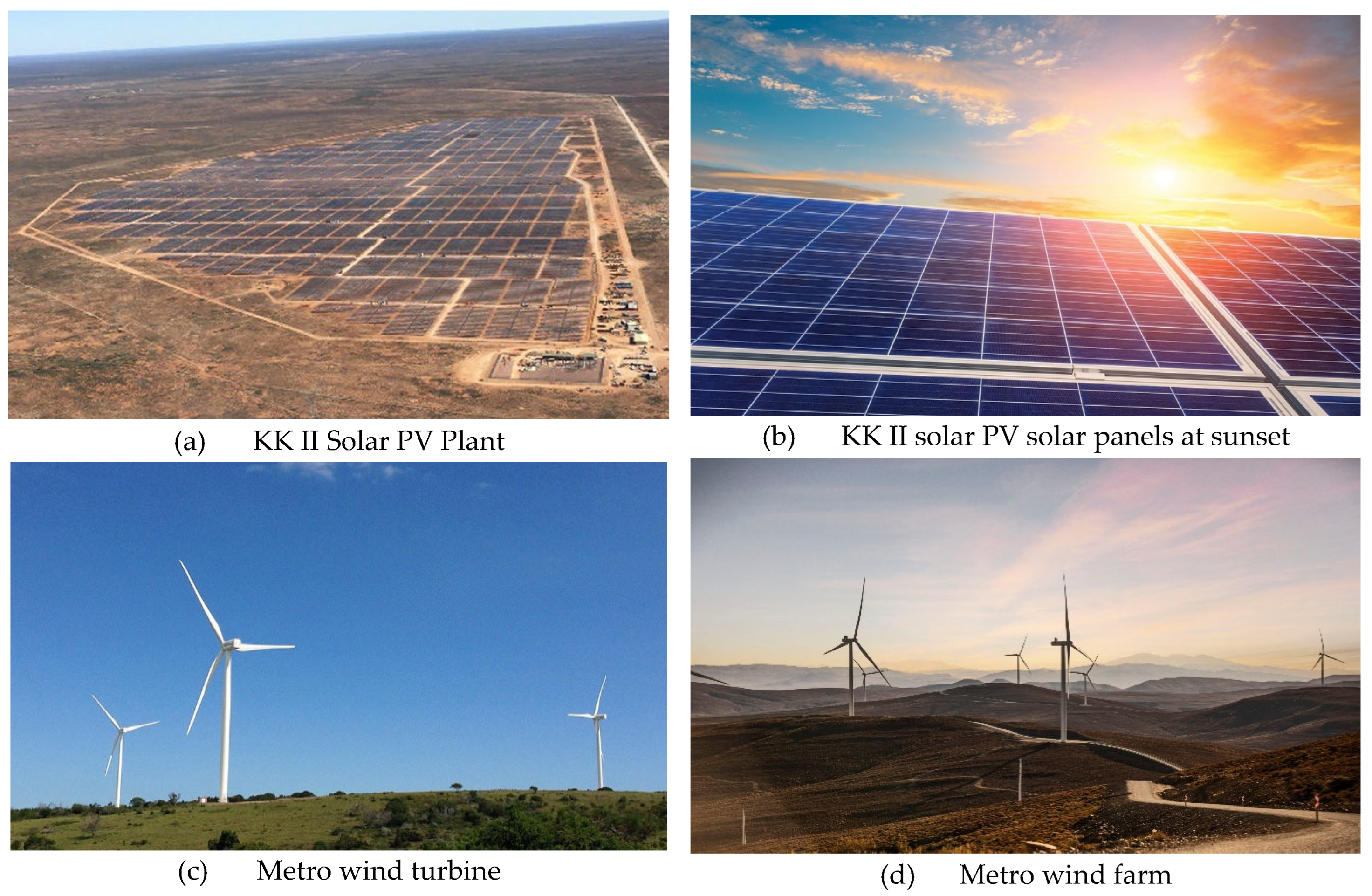
Figure 2.
Projected generation mix in SA. [source: draft integrated resource plan 2010-2050—South Africa Department of Energy].
Figure 2.
Projected generation mix in SA. [source: draft integrated resource plan 2010-2050—South Africa Department of Energy].
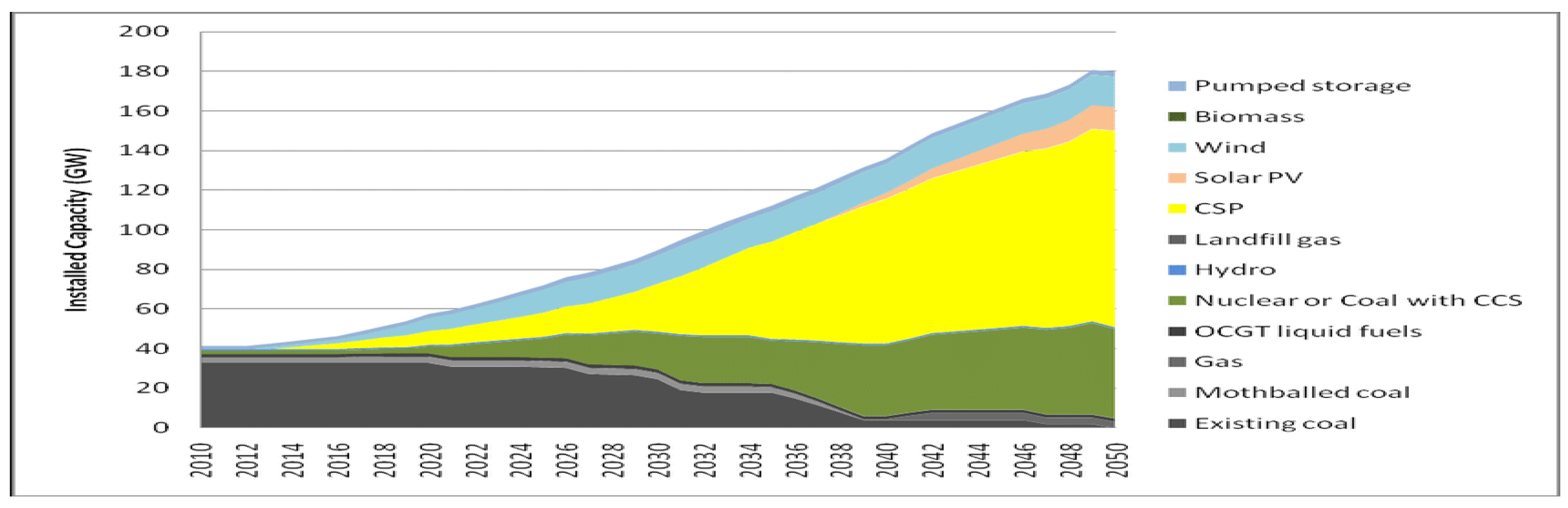
Figure 3.
Voltage levels.
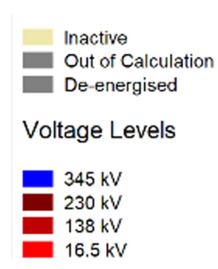
Figure 4.
KK II Solar PV Plant.
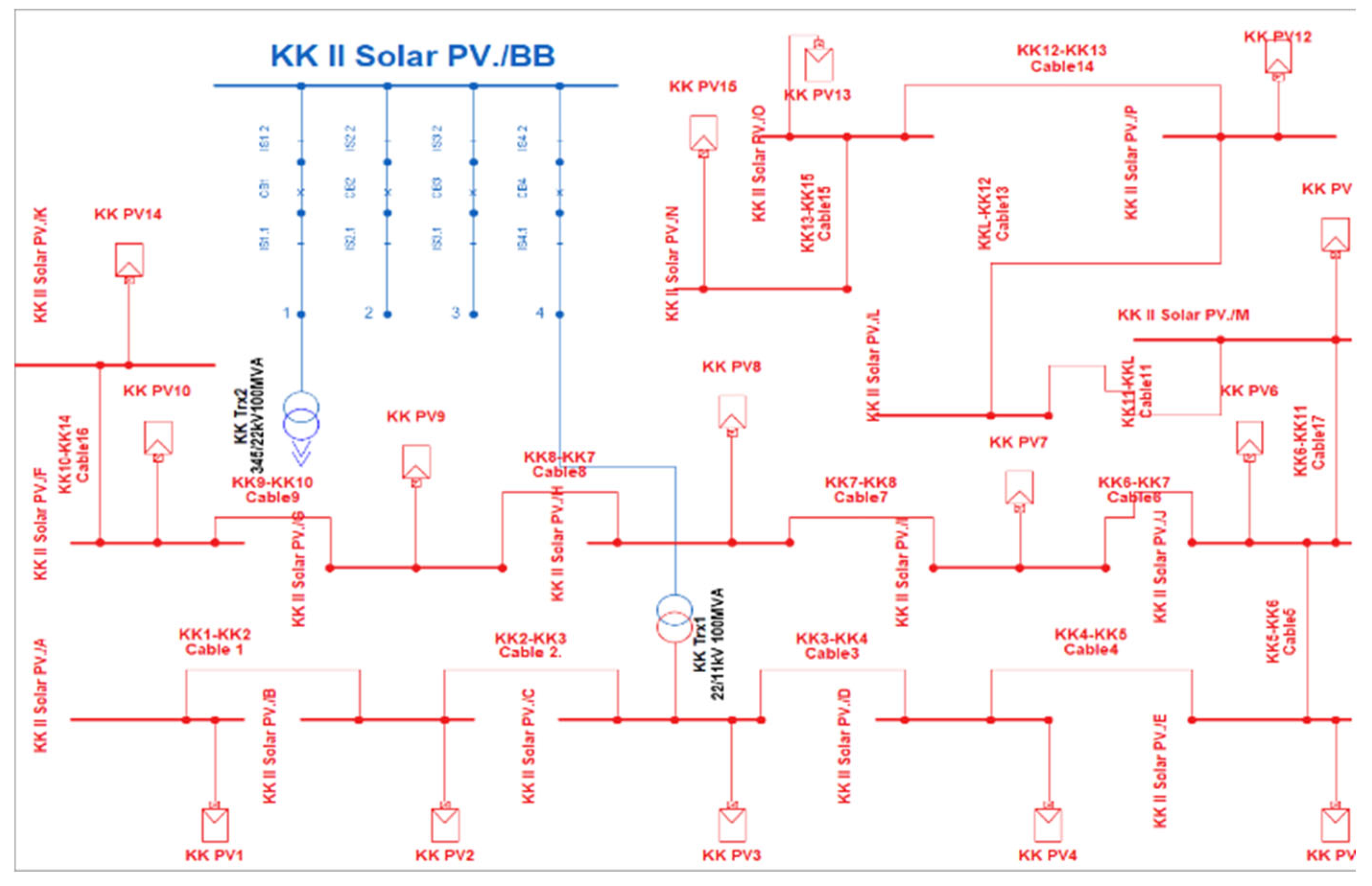
Figure 5.
Metro wind farm.
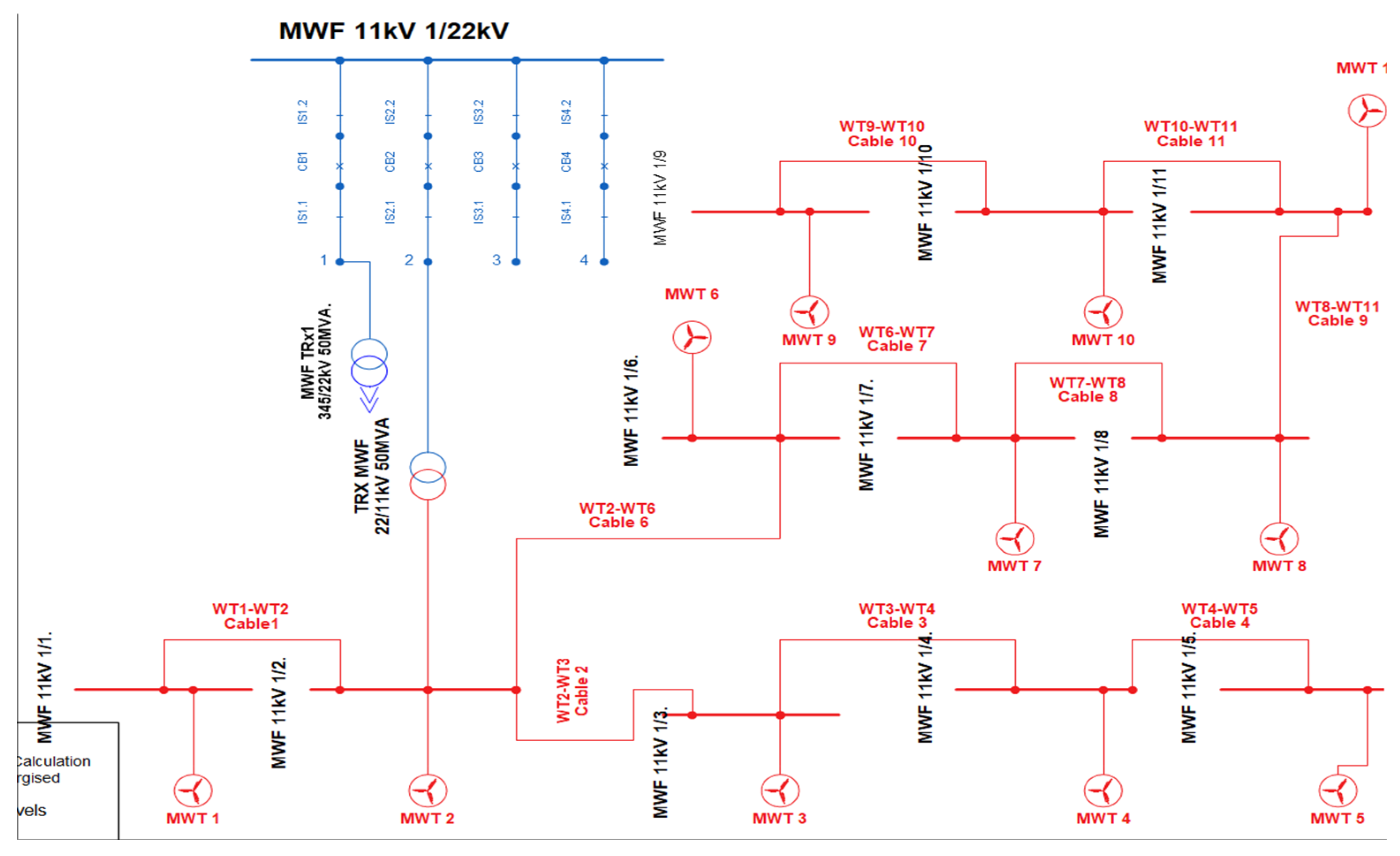
Figure 6.
Wind turbine speed.
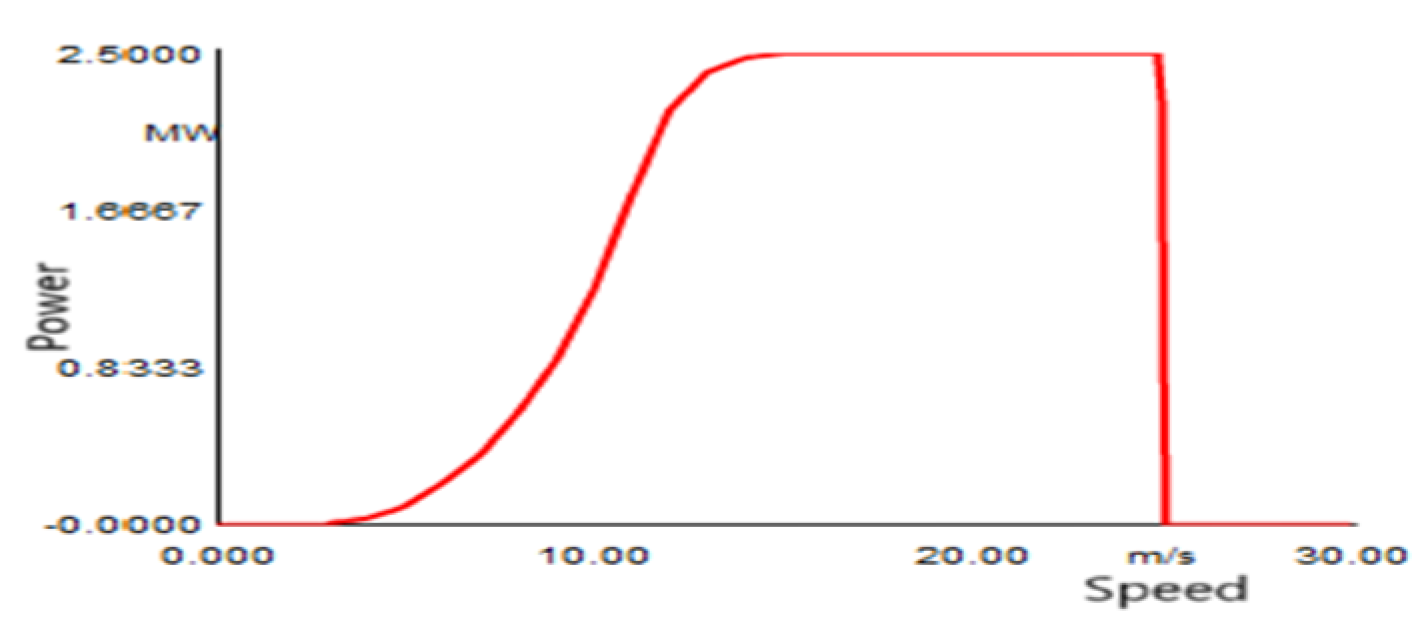
Figure 7.
Wind power capability curve.
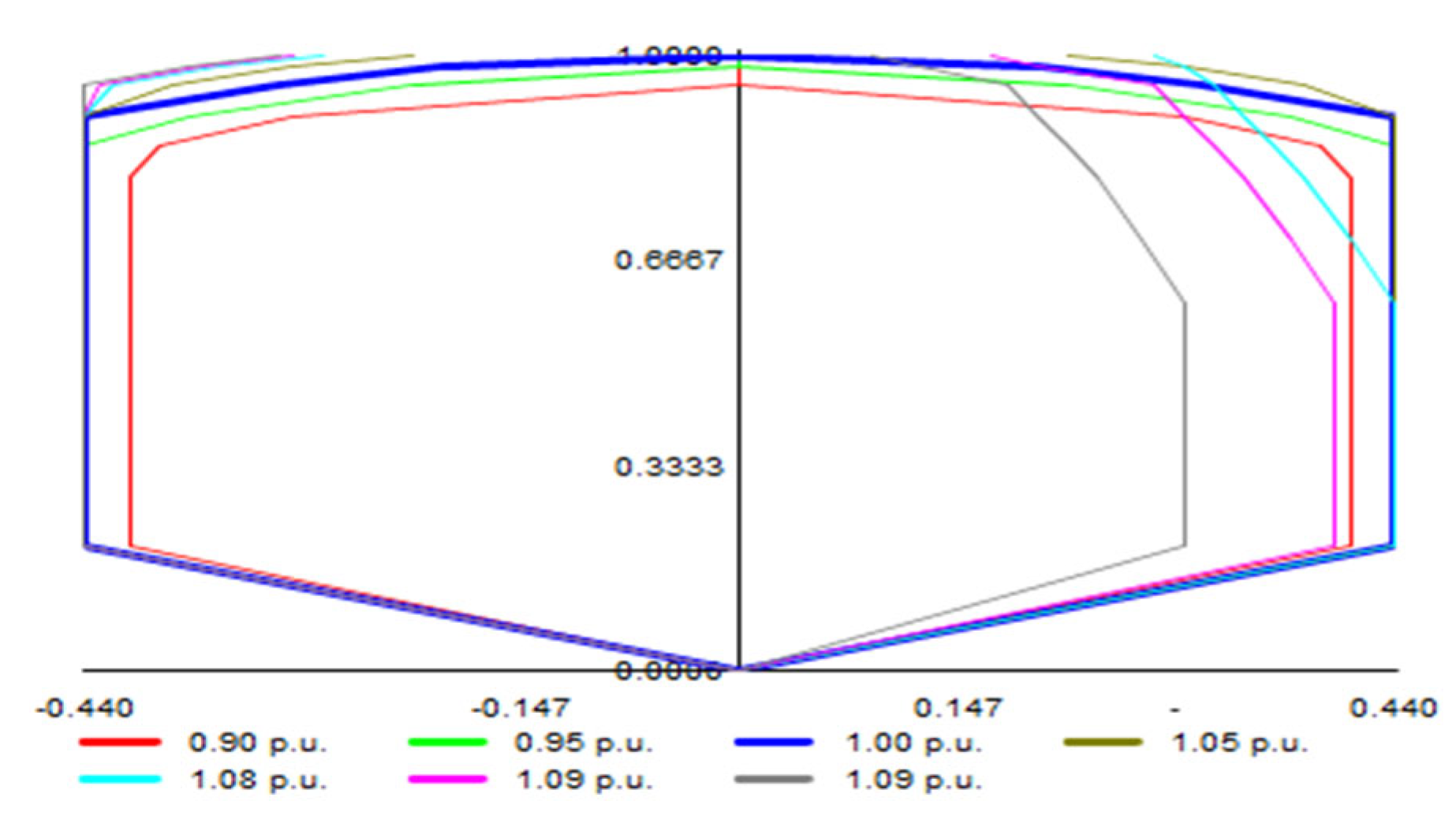
Figure 8.
Characteristic wind generator time.
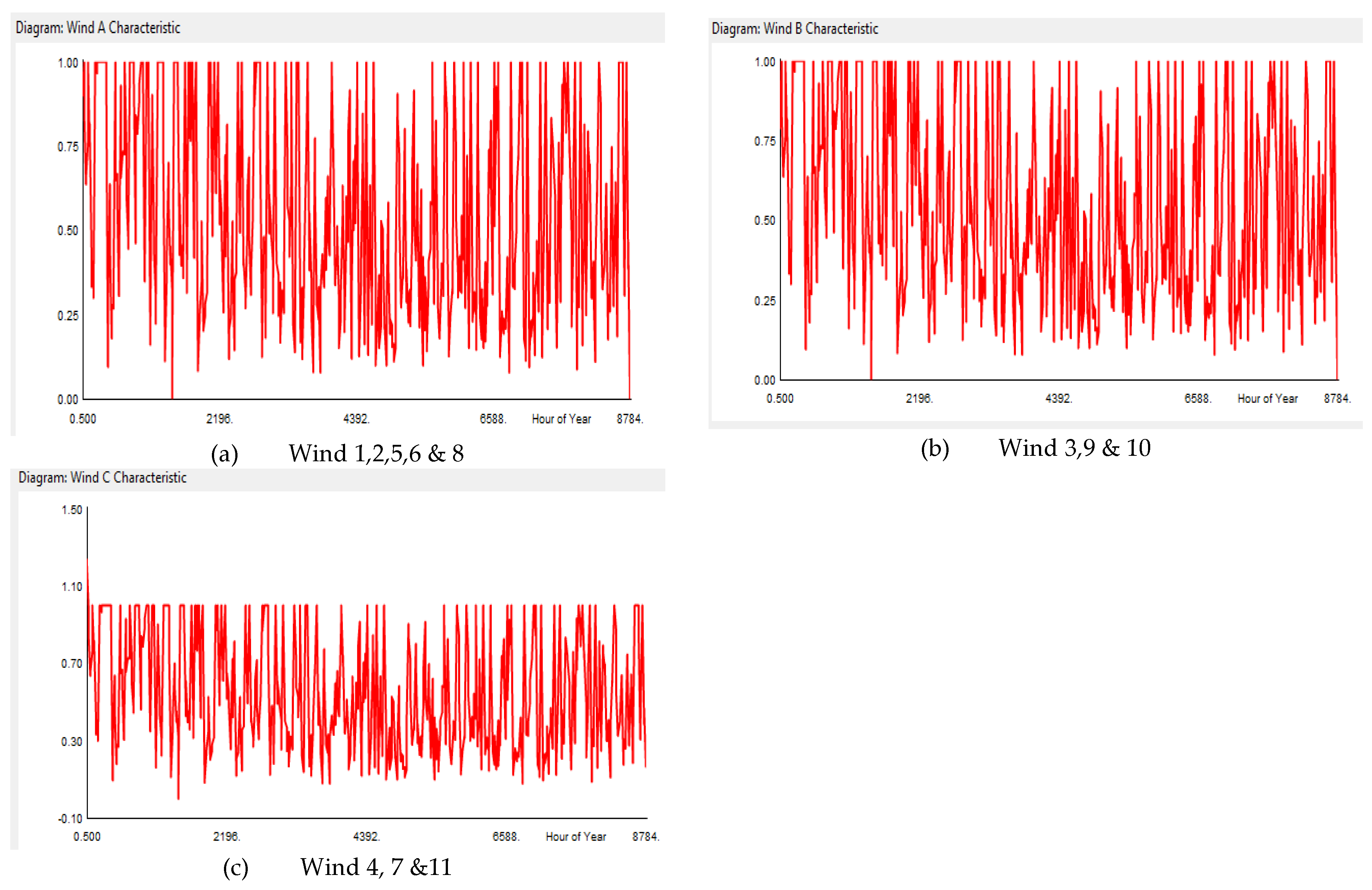
Figure 9.
Characteristic solar generator time.
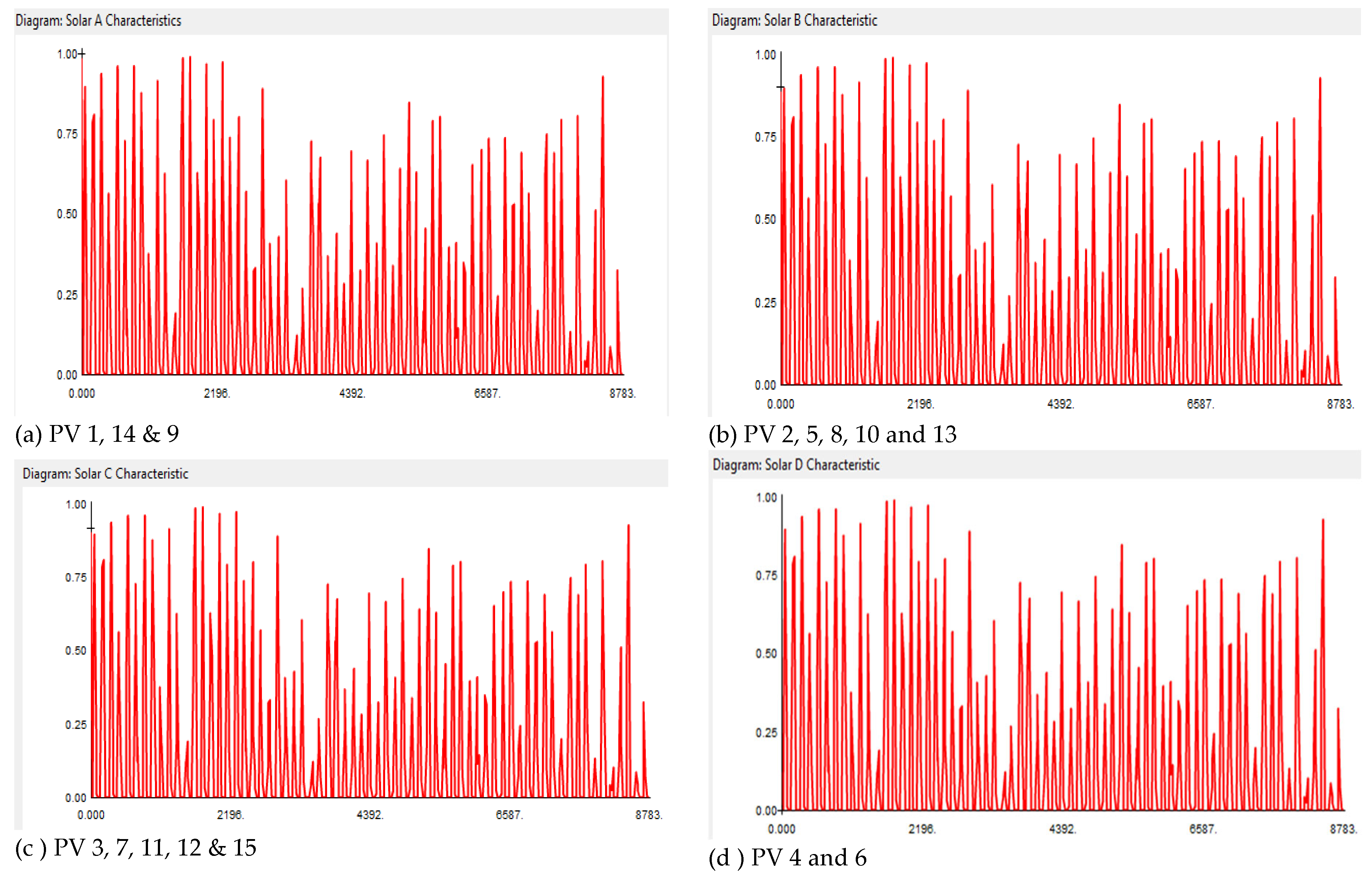
Figure 10.
distributed characteristics and wind speed correlation.
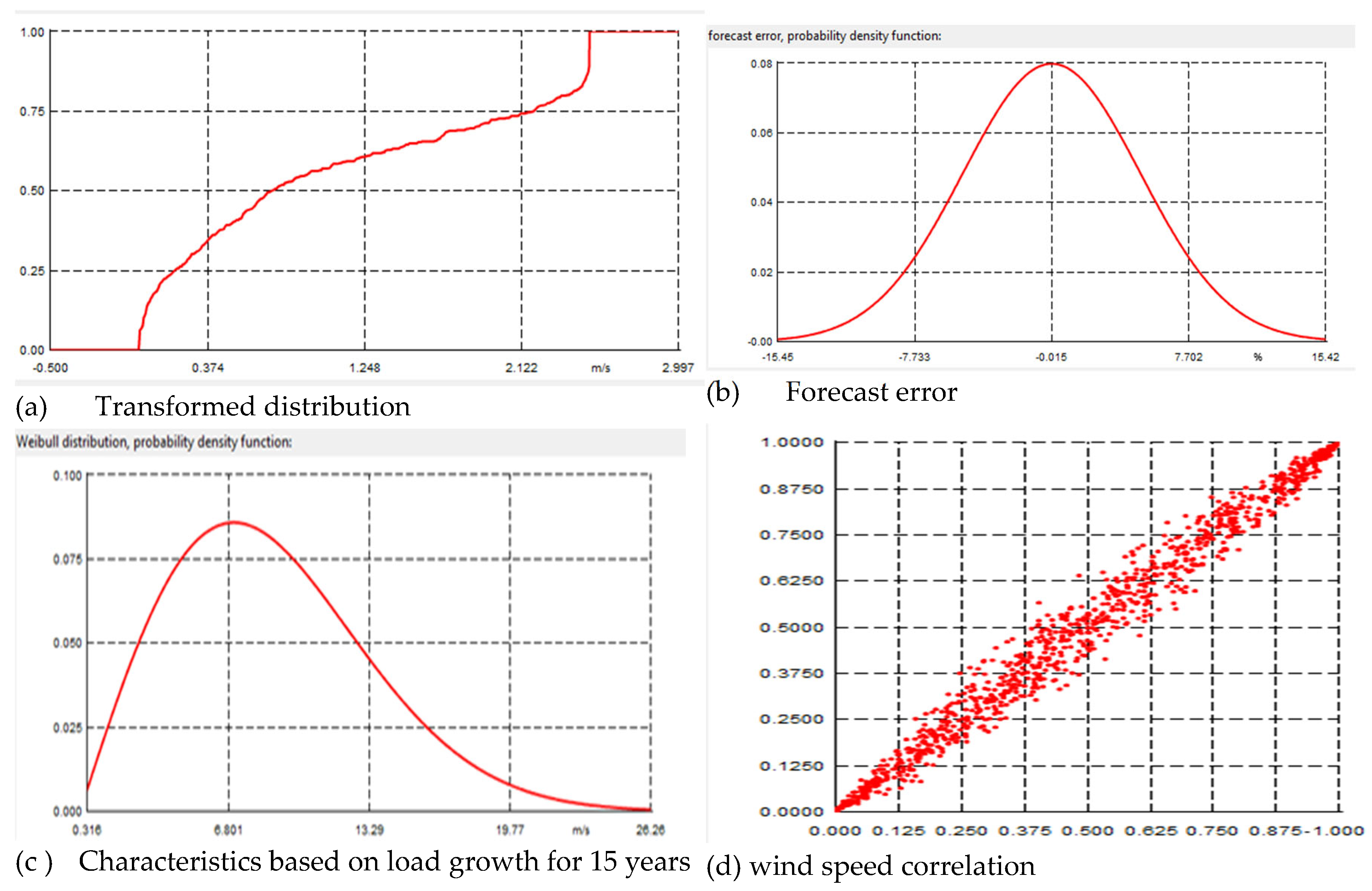
Figure 11.
Metro wind farm simulation network.
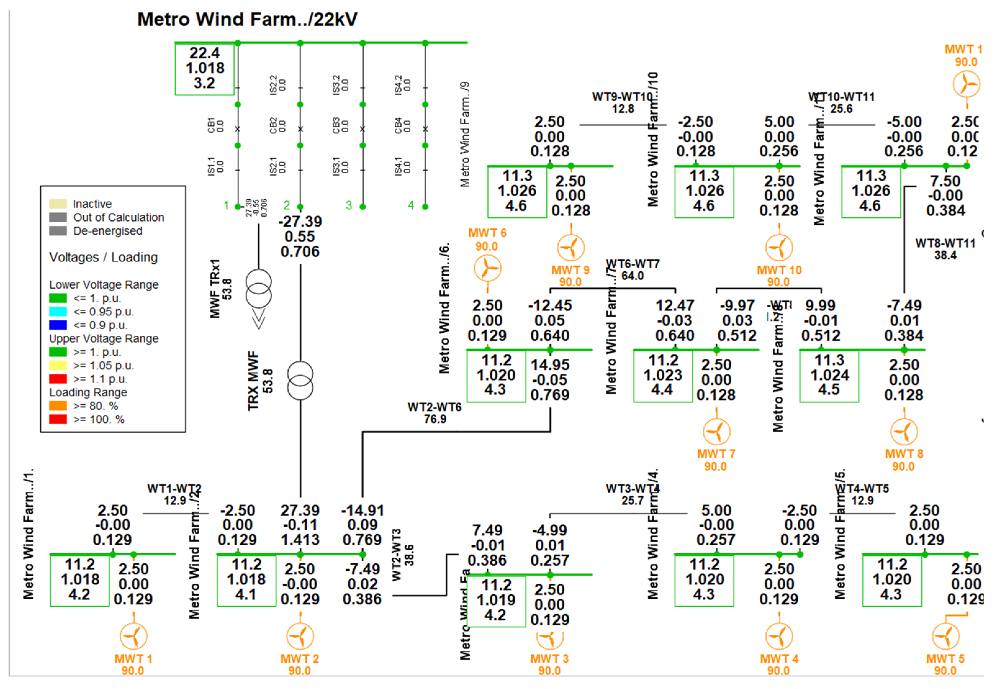
Figure 12.
KK II solar PV plant.
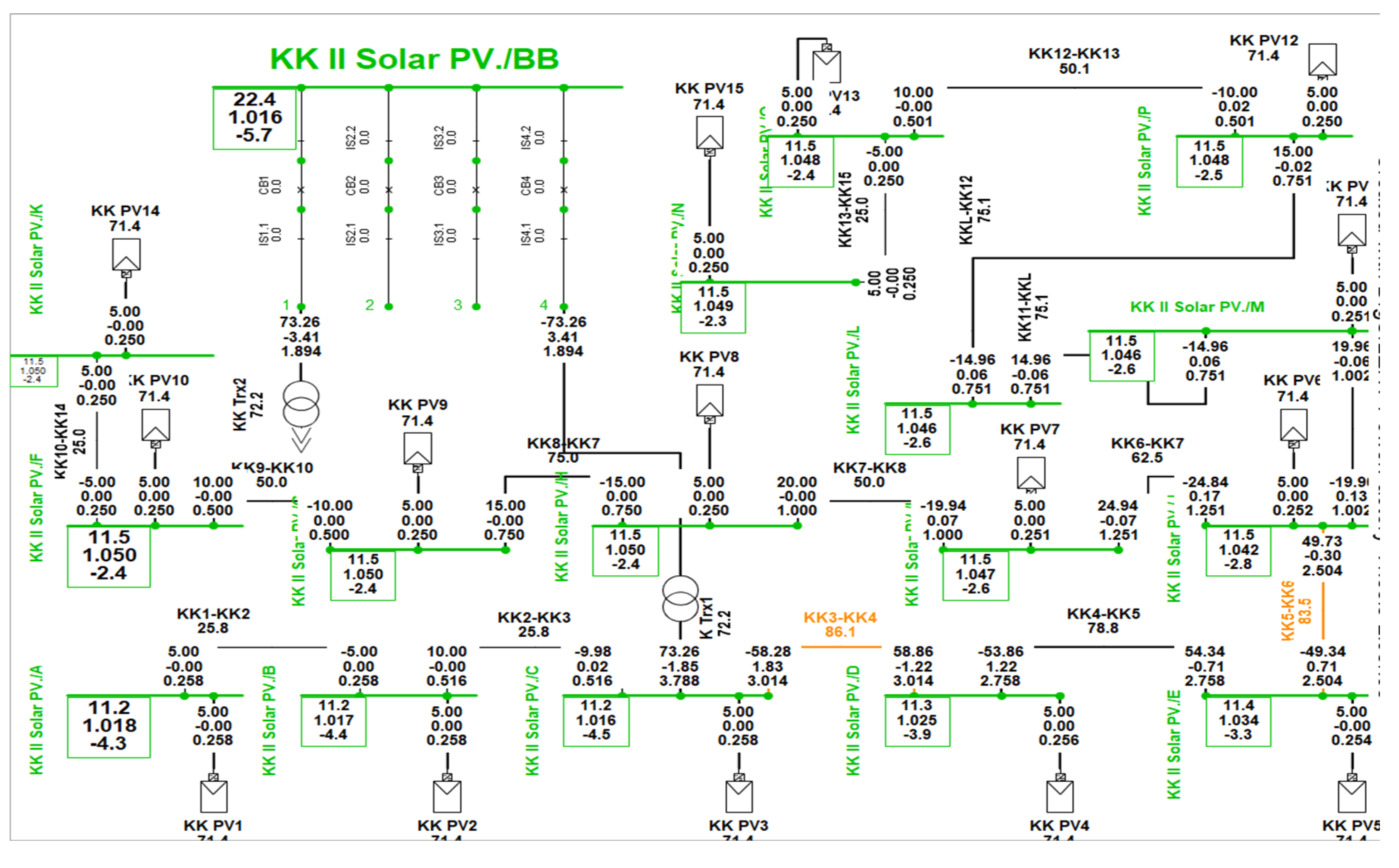
Figure 13.
KK II solar Busbar Voltage p.u for 1 year.
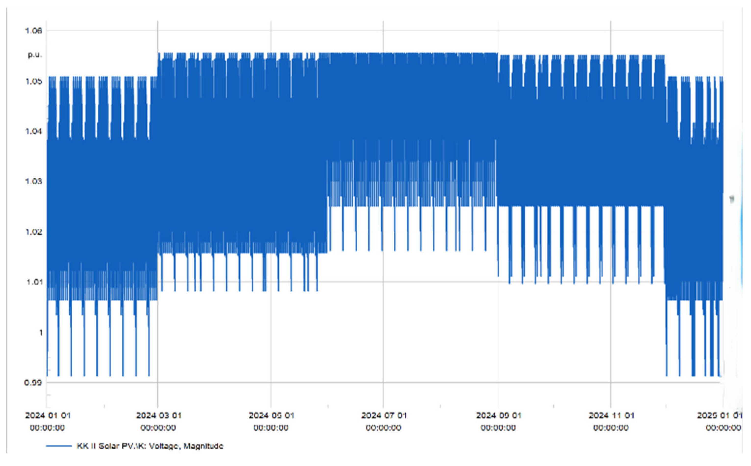
Figure 14.
Metro Wind Farm Under Quasi-Dynamic Simulation.
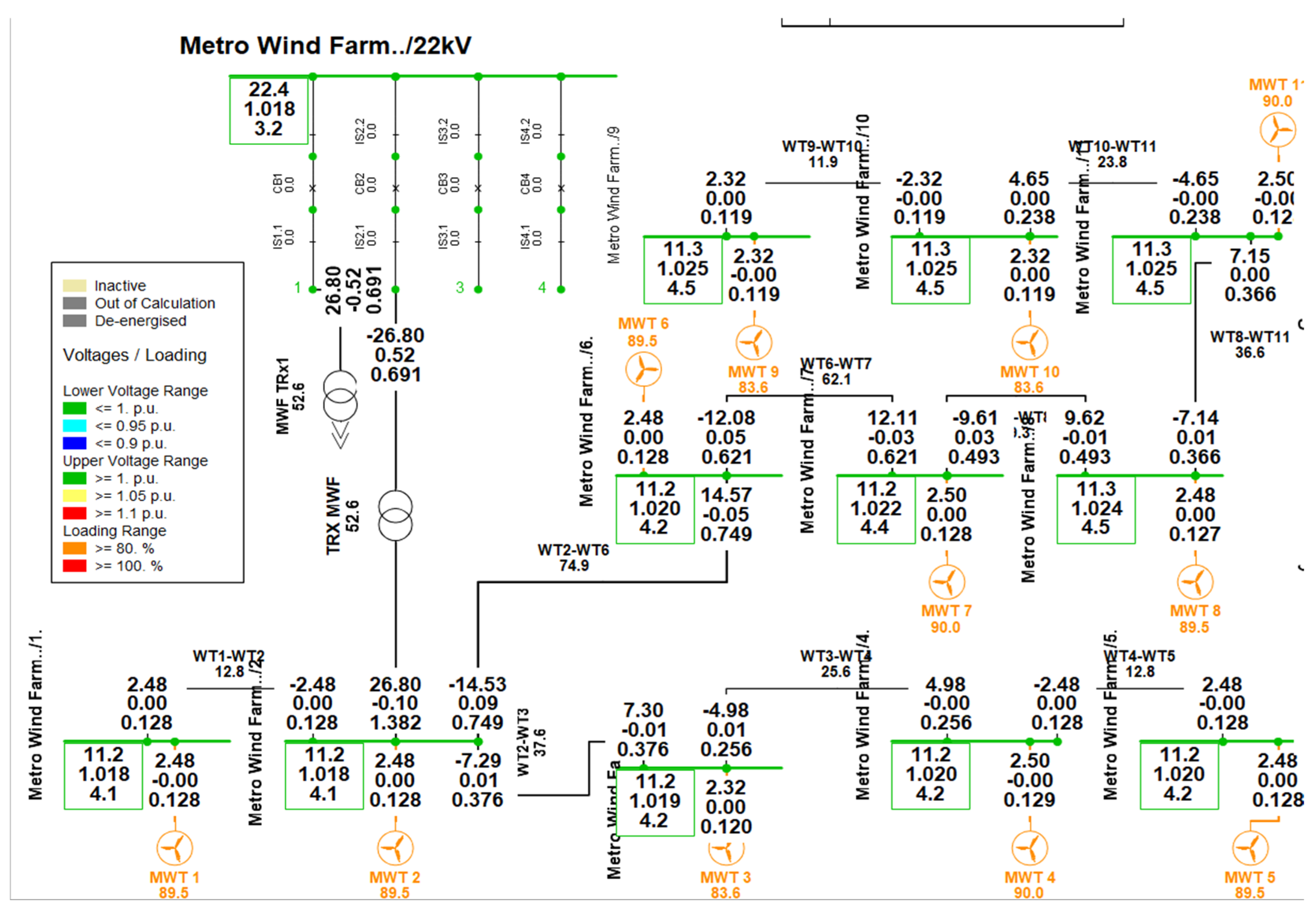
Figure 15.
KK II Solar PV Plant Under Quasi-Dynamic Simulation.
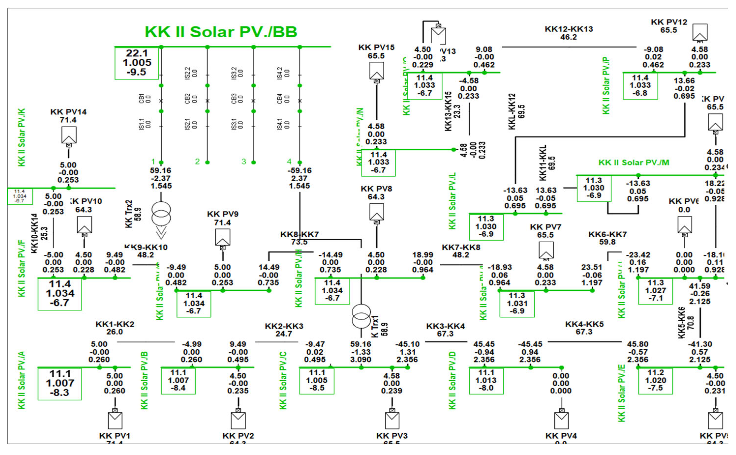
Figure 16.
KK II Solar PV Busbar Voltage (p.u) for 1 year under quasi-dynamic.
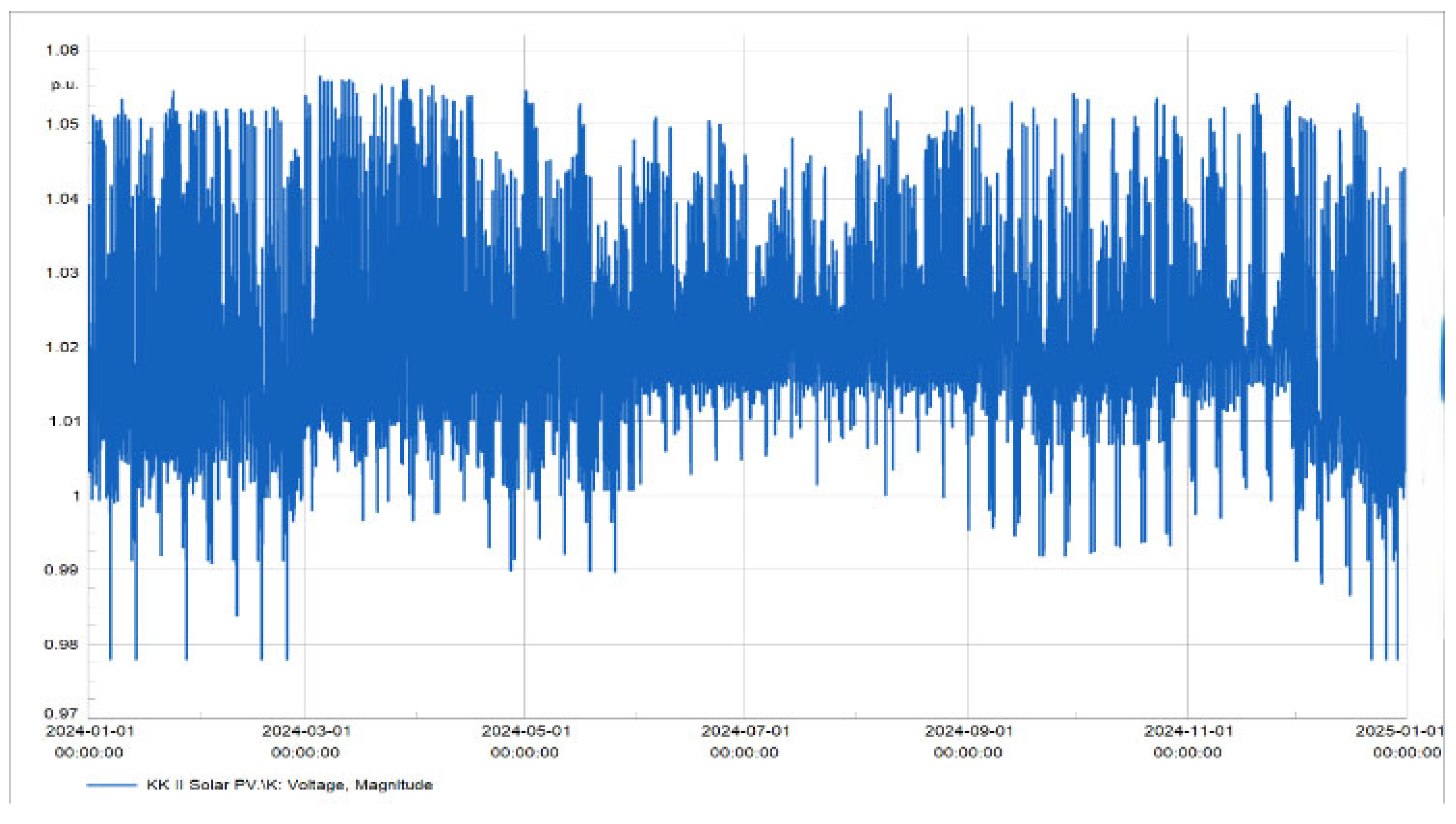
Figure 17.
Effect of Load growth over 5 year period.
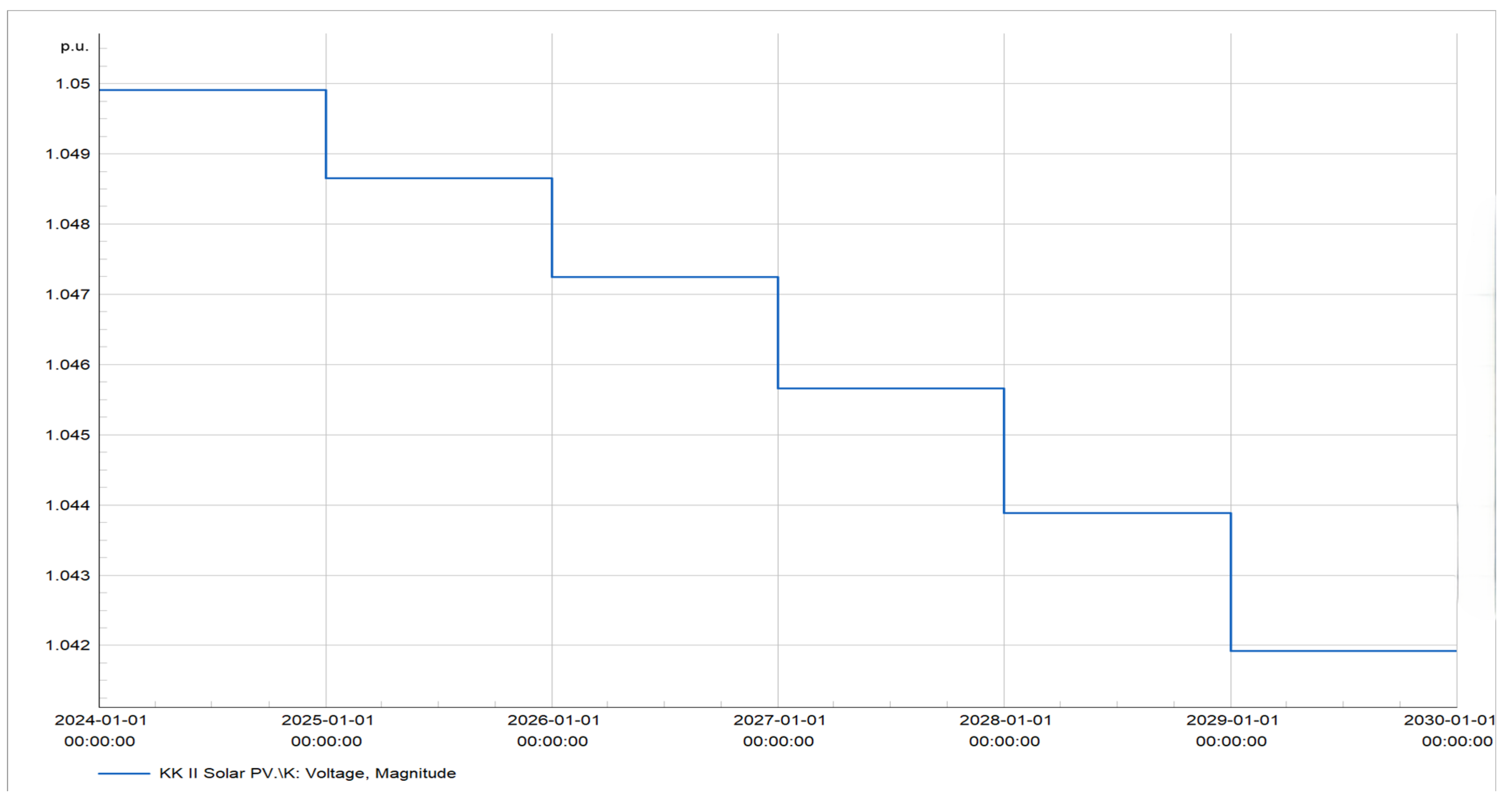
Figure 18.
KK II Solar PV Load forecast over 10 10-year period.
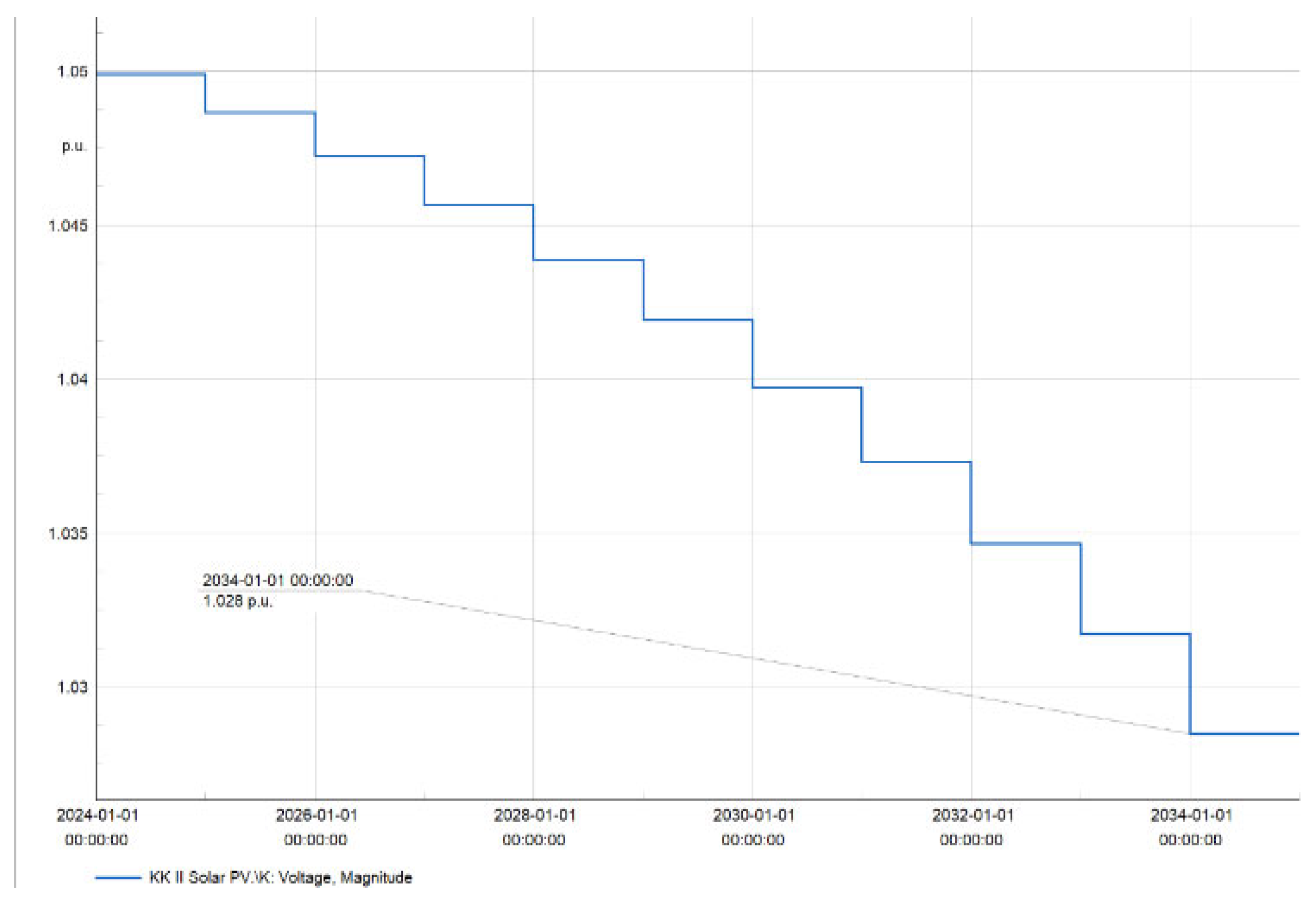
Figure 19.
Basic energy analysis results.
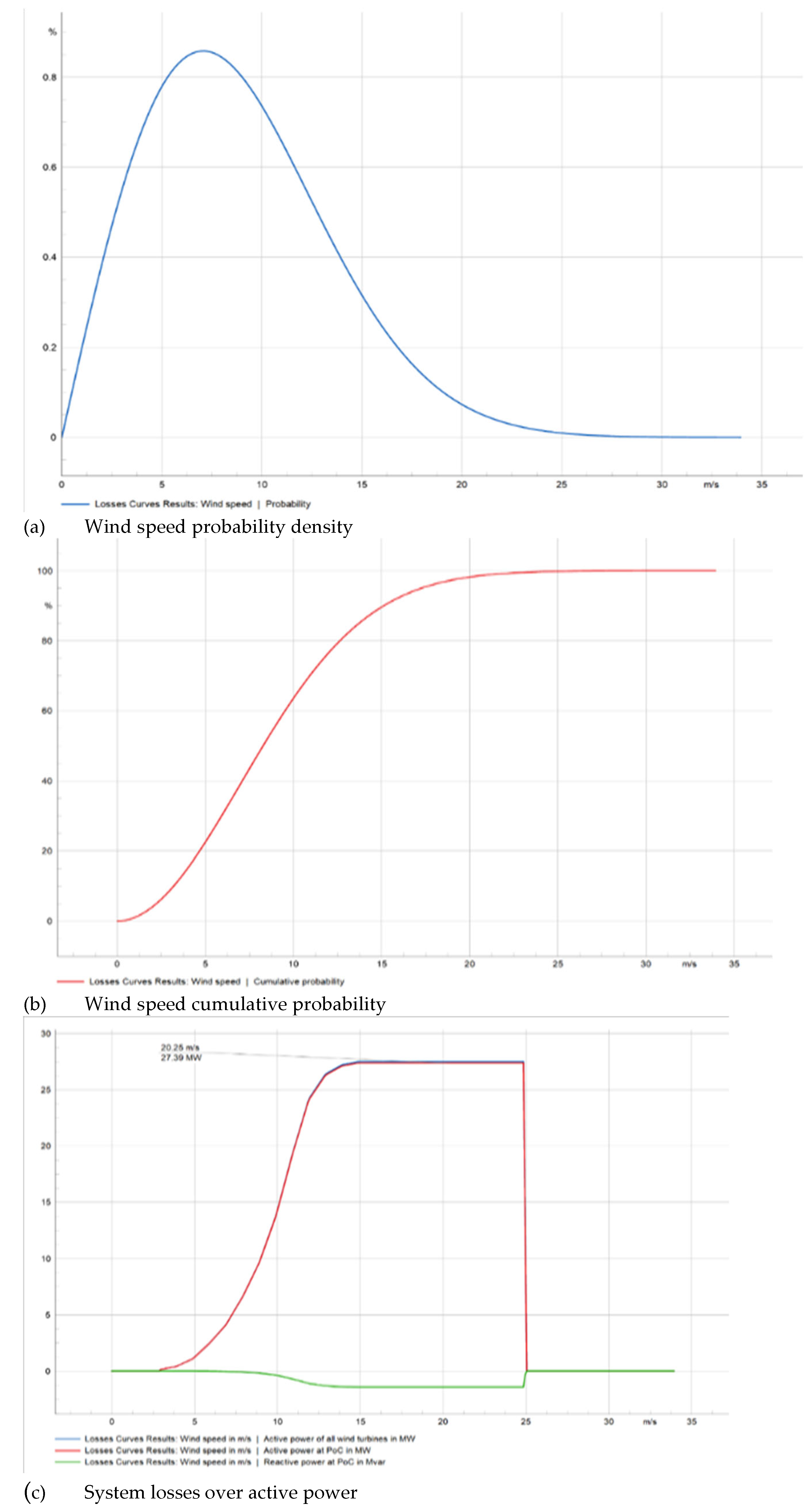
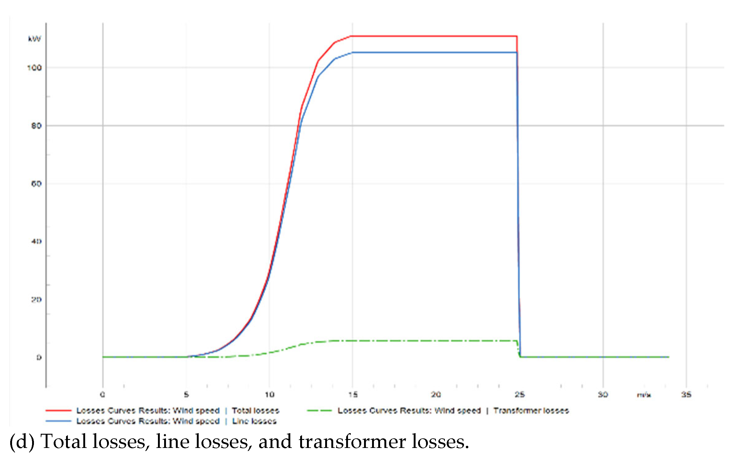
Figure 20.
Metro WF under Probabilistic analysis.
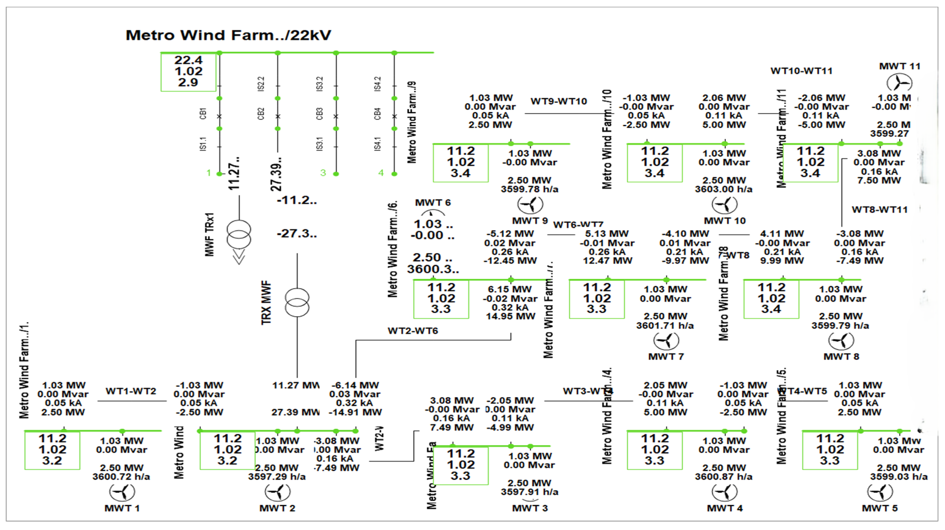
Figure 21.
Metro Wind Farm Annual load duration curve.
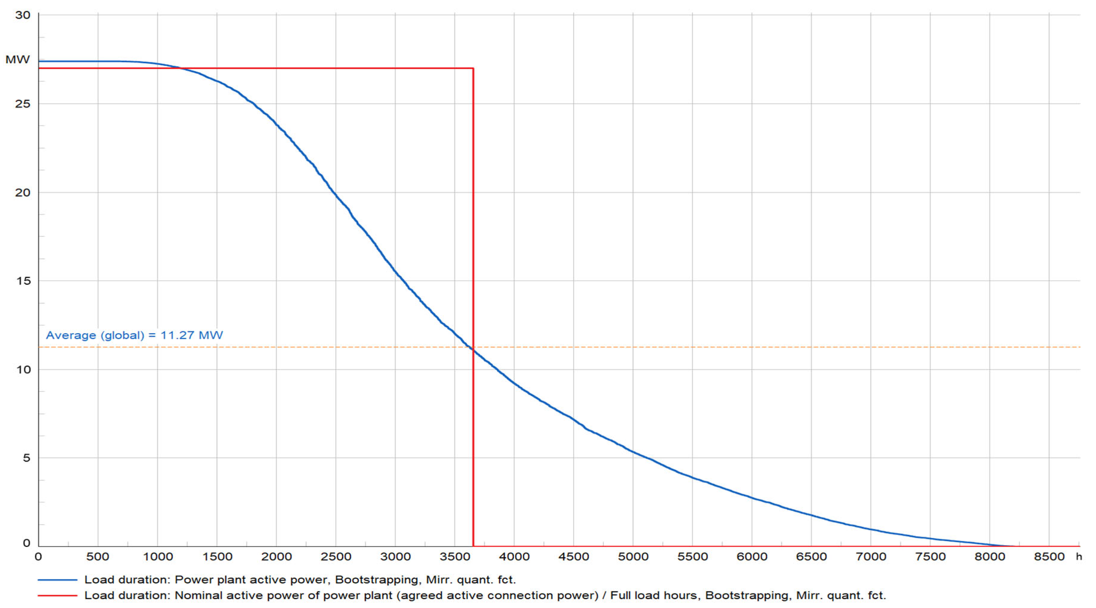

Table 1.
High RE Penetration Drivers.
| Name | Impact |
| Climate Change Mitigation [10]. | Increasing RE penetration is driven by greenhouse gas reduction. |
| Policy and Regulation [11,12]. | Government regulations, such as RE portfolio standards (RPS) and feed-in tariffs (FIT), have stimulated the expansion of renewable energy sources. |
| Cost Reductions [13]. | Recently, solar PV panels, wind turbines, and battery storage devices have become cheaper, making renewables more viable. |
| Technological Advancements [14]. | Power electronics, forecasting, and grid management innovations improve variable resource integration. |
Table 2.
South Africa’s Installed Power capacity.
| Installed power sources | Installed capacity (MW) | Installed capacity (%) |
| Thermal | 45489 | 78 |
| Gas | 2409 | 4 |
| Nuclear | 1840 | 3 |
| Wind | 2710 | 5 |
| Solar | 2323 | 4 |
| Hydro | 3393 | 6 |
Table 3.
RE concerns.
| Renewable Energy | Uncertainty |
| Solar [27]. | Local sun irradiance directly influences solar energy output, often managed by Beta. |
| Wind [28]. | Wind velocity directly influences wind energy production, commonly modeled using the Weibull distribution. |
| Hydro [29]. | Hydrological and hydraulic conditions influence hydropower plant production. |
Table 4.
Weibull curve parameters.
| Parameter | Value |
| Scale factor | 10m/s |
| Shape factor | 2 |
| Confidence level | 0.99999 |
| Wind speed step size | 0.1m/s |
Table 5.
Basic analysis of the wind farm.
| Basic Analysis | |
| Average power of power park over a year | 11.3MW |
| Total annual net energy output at PoC | 98745MWh |
| Total Average electrical energy losses per year | 305.2MWh |
| Number of hours of the power park full load operation | 3668.5267 h |
| Loss of profit due to losses in feed-in operation | 15261.84 USD |
| profit | 4937249.24 |
Table 6.
probabilistic analysis of the wind farm.
| Probabilistic Analysis | |
| Average power over a year | 11.27MW |
| Annual generation | 99007.2 MWh |
| Annual energy yield | 98703.9 MWh |
| Total Average Electrical energy losses per year | 303.3 MWh |
| Number of hours of power park full load operation | 3655.7001 h |
| Electrical losses (Price) | 15163.29 USD |
| Profit | 4935195.16 USD |
Disclaimer/Publisher’s Note: The statements, opinions and data contained in all publications are solely those of the individual author(s) and contributor(s) and not of MDPI and/or the editor(s). MDPI and/or the editor(s) disclaim responsibility for any injury to people or property resulting from any ideas, methods, instructions or products referred to in the content. |
© 2025 by the authors. Licensee MDPI, Basel, Switzerland. This article is an open access article distributed under the terms and conditions of the Creative Commons Attribution (CC BY) license (http://creativecommons.org/licenses/by/4.0/).
Copyright: This open access article is published under a Creative Commons CC BY 4.0 license, which permit the free download, distribution, and reuse, provided that the author and preprint are cited in any reuse.


