Submitted:
15 July 2025
Posted:
16 July 2025
You are already at the latest version
Abstract
Microplastic (MP) analysis via microspectroscopy typically examines only 1-10% of filter substrates due to time constraints, requiring reliable extrapolation methods for quantitative environmental monitoring. Current subsampling strategies suffer from heterogeneous particle dispersion, leading to 50-80% error in MP quantification. Additionally, MP researchers require enhanced environmental MP mass datasets, necessitating reliable conversion algorithms from two-dimensional morphological data to mass estimates. This study introduces an area-based extrapolation technique that compares the MP-to-generic particle area ratio within a rectangular field of view against total particle area on the entire filter membrane, combined with a simplified morphology-to-mass conversion model (Hagelskjær model). First, two Sphagnum moss samples were analyzed using Raman microspectroscopy and critical angle darkfield illumination microscopy. Results demonstrated stable MP concentrations (17% RSD [n = 8]) despite heterogeneous generic particle distribution (31% RSD [n = 8]), with mean particle-area coverage of 2.4% per subsample. Then, twenty MP fragment subsamples (10 µm to 1500 µm) were used to calibrate the height multiplier (Mh) which ranged from 0.26 to 0.47 (mean: 0.34 ± 0.05, 15% RSD), establishing that particle height equals approximately one-third of the minimum Feret diameter with this simplified plane-particle model. These methods enable MP quantification and mass estimation from limited spectroscopic analysis.
Keywords:
Raman microspectroscopy
; environmental monitoring
; particle distribution
; mass estimation
; subsample analysis
1. Introduction
Microplastics (MPs) are synthetic polymer particles that measure between 1 µm to 5 mm on their largest axis. When conducting microspectroscopic analysis for quantitative identification of MPs in the smallest size range, often only a small percentage of the filter substrate can be examined due to time constraints [1,2,3]. Even when n >20,000 individual particles are analyzed over a 24-hour period using Raman microspectroscopy, only 2-3% of the total filter area can be investigated [4,5]. Current Raman microspectroscopy subsampling strategies measure about 1 to 10% of the filter area [6].
Simplified extrapolation based on upscaling the analyzed fraction of a rectangular field of view (FOV) is unprecise because particle dispersion on a filter membrane is often heterogenous [6,7]. To correct for heterogenous particle dispersion by collecting data that is representative of the complete filter membrane, spectral acquisition techniques including wedge-shaped analysis [1], random particle selection [8] as well as spirals and crosses [9], have been developed. These methods all rely on adjusting data-sampling parameters to achieve statistically reliable MP content extrapolation based solely on the analyzed fraction.
However, particle count extrapolation represents only one component of comprehensive MP analysis. While accurate extrapolation of MP particle numbers addresses one analytical challenge, reliable conversion methods from morphological data to mass estimates are essential for comprehensive environmental monitoring [10,11,12]. Because spectroscopic techniques dominate current MP analysis workflows [13,14,15], reliable conversion formulas that transform two-dimensional morphological data into mass estimates are needed. Most existing models estimate the volume of a particle by assuming a known three-dimensional geometric shape based on observed metrics such as area and size [16,17,18,19]. However, the irregular nature of environmental MP fragments makes it challenging to apply standardized geometric models consistently across diverse samples.
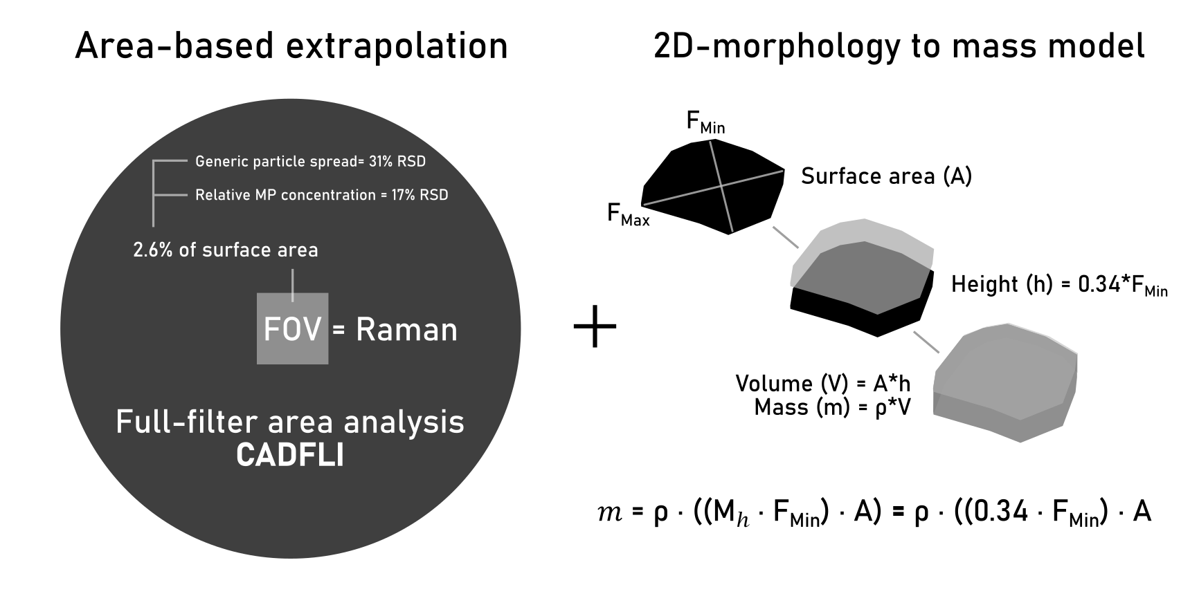
To address these issues, we present two novel approaches for particle count extrapolation and conversion from counts to mass. First, we developed a novel extrapolation approach that compares the ratio of generic particle area to MP distribution, within a single rectangular FOV against the total generic particle area across the complete filter membrane. Second, we present a simplified plane-particle model (Hagelskjær model) to calculate the volume of a particle using two observable parameters: i) surface area, and ii) minimum Feret diameter. The conversion formula uses a constant multiplier value to determine particle height, calibrated on observations presented in this study. This simple model relies on the principle that for a three-dimensional detached object perceived in two dimensions, the observed lateral dimensions (y- and x-axis) are likely superior in length, in comparison to the forward direction (z-axis) when the particle is in a resting state. This is because the gravitational force guides the particle towards a state of stable equilibrium, which is unlikely to be the shortest dimension [20], unless otherwise affected by surface adhesion not accounted for in this study.
These two combined methodologies aim to enable accurate extrapolation of MP counts and mass conversion from limited spectroscopic analysis of small FOVs, facilitating efficient monitoring of large environmental datasets while maintaining analytical precision and reducing time constraints inherent to current microspectroscopic workflows
2. Methods and Materials
2.1. Particle-Area Based Extrapolation
2.1.1. Experimental Setup
Two Sphagnum moss samples collected in France (sample A and sample B, respectively), were manipulated according to the complete purged air-assisted digestion and density separation protocol [5]. The final MP-enriched analyte was vacuum filtered onto two individual aluminium oxide filter membranes [pore size: 0.1 µm, filter diameter: 25 mm] (Anodisc, Whatman, England). The diameter of the filtered area was restricted by the width of the glass filtration funnel, measuring 14 mm in diameter. On each of the two filter membranes, four individual 4 mm² square FOVs were analyzed by Raman microspectroscopy, following the pattern visualized in Figure 1. Between the individual samples, the total number and surface area of MPs and generic particles, as well as the relative size and polymer type distributions within the four FOVs were compared.
2.1.2. Raman Microspectroscopy
A 4 mm2 square FOV was analyzed by stitching 1666 micrographs into a high-resolution mosaic at a spatial resolution of 0.3 µm/pixel. Particles measuring ≥2 µm in area-equivalent diameter (circular model) were subject to µRaman analysis. Measurements were carried out at 20°C using a Horiba LabRAM Soleil (Jobin Yvon, France). The samples were excited at 8% (7.2 mW) power output with a high stability air-cooled He–Cd 532 nm laser diode utilizing a Nikon LV-NUd5 100x objective. The lateral resolution of the unpolarized confocal laser beam was on the order of 1 µm. Spectra were generated in the range of 200–3400 cm−1 using a 600 grooves/cm grating with a 100 µm split. The spectral resolution was on the order of 1 cm−1. Particles within each mosaic, constructed using the LabSpec6 (LS6) SmartView configuration, were analyzed using the Particle Finder application V2. LS6 SmartView determines the topography (± 50 µm) and saves the focal point of all particles on the captured micrograph, enabling the stage to rapidly move the relevant particle into focus. The micrograph is converted into an 8-bit 0–255 greyscale image in which parameters are set by the user to visually separate particles from the darker filter substrate. Each particle was analyzed for 1 s by 2 accumulations at the above-described settings.
2.1.3. Spectral Matching and Verification
Using the Spectragryph spectral analysis software V1.2.17d (Dr. Friedrich Menges SoftwareEntwicklung, www.effemm2.de/spectragryph), all raw spectra were processed using adaptive baseline correction with 15% coarseness. The processed spectra were cross-referenced for their entire spectral range, using our in-house library containing selected spectra from the SLoPP and SLoPP-E [21] and the Cabernard [22] spectral libraries, also including self-obtained in-house polymer spectra. Spectral matches were denominated by hit quality index (HQI)-values from 0 to 100% match. Spectra rated above 65% HQI were considered MP candidates and were manually inspected and sorted by a trained interpreter to determine their validity. Additionally, unintentionally partitioned MP particles (edge particles) were merged using a dedicated merging tool [4].
2.1.4. Full-Filter Particle-Area Estimation
Critical angle darkfield illumination (CADFLI) microscopy (ColSpec® MK2, LightForm, Inc., USA) was used to capture multiple micrographs at a spatial resolution of 2.6 µm/pixel. 28 micrographs were merged using the Grid/collection stitching tool [23] to construct mosaics displaying the entire filter membrane. CADFLI microscopy enables the visual elimination of the filter substrate to isolate the residual particles, providing an effective means of estimating the total particle-area on the filter membrane (Figure 2).
2.2. Two-Dimensional Particle Morphology to Mass Conversion Model
2.2.1. Experimental Setup
The current MP fragments, produced through cryomilling and cascade sieving [24,25]. in dry, neat (powder) format (EasyMP™, Microplastic Solution, France) were used in this experiment:
- Sample 1: polystyrene (PS) (500-1500 µm), Blue.
- Sample 2: polypropylene (PP) (100-500 µm), Red.
- Sample 3: polyethylene (PE) (10-200 µm), Blue.
- Sample 4: polypropylene (PP) (10-200 µm), Clear/transparent.
- Sample 5: polyethylene (PE) (10-100 µm), Green.
For each sample, four subsamples were prepared. The total dry mass of each sample was determined using a PCE-ABT 220L balance (PCE instruments, Germany). The dry mass of samples 2-5 were determined at 52.1 mg, 9.8 mg, 3.8 mg, and 5.4 mg, respectively. The powders were weighed in glass pipette bottles (Oputec, Germany) and were suspended in either 30, 50- or 100-mL ethanol (95 vol.%), adapted to the quantity of MP powder to avoid filter saturation. For each sample, four subsamples between 0.5 to 1.0 mL were pipetted onto 25 mm filter membranes to capture photomicrographs via CADFLI microscopy. The mass of individual subsamples followed the current logic, using sample 2 as an example:
Dry MP powder mass: 52.1 mg (52 100 µg) → MP Powder suspended in 50 mL ethanol (95 vol.%) solution → 1 mL solution containing 1042 µg MP powder (52 100 µg / 50 = 1042 µg) filtered onto 25 mm membrane for CADFLI microscopic analysis.
The applied dosing method represents a mean relative standard deviation (RSD) of 10% (n = 5) [24] not accounted for in this study. The comparatively larger particle size range of sample 1 allowed for the weighing of individual subsamples, where subsamples 1-4 weighed 17.4 mg, 20.4 mg, 14.0 mg, and 23.4 mg, respectively.
2.2.2. Particle Segmentation and Mass Conversion
CADFLI microscopy was applied to capture images of the individual subsamples for visual segmentation of the reference MP fragments. Depending on the image resolution, 28 to 50 micrographs at a spatial resolution from 2.0 to 2.6 µm/pixel were merged using the Grid/collection stitching tool [23] to construct mosaics displaying the entire filter membrane (Figure 3).
This study presents a particle morphology to mass conversion formula (Hagelskjær model) where particle volume, and incidentally mass, is calculated on the basis of two observable 2D parameters: surface area (A), and minimum Feret diameter (FMin). The volume (V) is calculated as the area of the particle multiplied by its height (h). Following the assumption that the observed lateral dimensions (y- and x-axis) are likely superior in length in comparison to the forward direction (z-axis or height), h is calculated as FMin multiplied by the height multiplier (Figure 4). Mh is calibrated on the basis of the weighed mass of samples 1, 2, 3, 4 and 5
Mass (m) is calculated by multiplying V by the specific gravity (ρ) of the polymer type in question, as per Eq 1:
To calculate the optimal height multiplier for fragments, Mh was initially set to 1, which assumes particle height (h) equals the minimum Feret axis (FMin). The ratio of weighed mass to the sum of calculated mass of all particles in the subsample determined the calibrated Mh for each individual subsample, as per Eq. 2.
3. Results and Discussion
3.1. Particle-Area Based Extrapolation
3.1.1. Sample-A
Within FOVs 1-4, a total of n = 7087, 16 754, 18 850, and 20 023 particles > 2 µm in area-equivalent diameter were segmented and analyzed by Raman microspectroscopy, respectively (Table 1). Here, n = 412, 751, 899, and 699 particles were identified as MPs, corresponding to 5.8%, 4.5%, 4.8% and 3.5% of the particle distribution, respectively. Although the total number of particles within individual FOVs varied by as much as n = 15 679 ± 5097 (33% RSD) (n = 4) the mean concentration of MPs remained more stable at 4.6% ± 0.8 (n = 4) (RSD = 18%).
The particle-area on the complete filter membrane was determined at 22.52 mm². Resultantly, FOVs 1-4 covered 2.84%, 2.01%, 2.85%, and 2.80% of the total particle-area, respectively, resulting in a mean particle-area coverage of 2.2% ± 0.72 per subsample.
Between the four investigated FOVs, the polymer type distribution remained consistent, with polyethylene (PE) making up 95.2% ± 1.1 (n = 4) of the polymer type distribution, followed by polyurethane (PU) at 2.0% ± 0.6 (n = 4) (Figure 5). Only 5 out of 12 detected polymer types were found in all four FOVs. Polymer types that comprised > 0.5% of the relative distribution were detected in all four FOVs. The particle size distribution of detected MPs across the four FOVs remained stable with RSD values below 20% in most size groups.
3.1.2. Sample-B
Within FOVs 1-4, a total of n = 23 890, 13 616, 23 234, and 12 662 particles > 2 µm in area-equivalent diameter were segmented and analyzed by Raman microspectroscopy, respectively (Table 2). Here, n = 612, 364, 403, and 302 particles were identified as MPs, corresponding to 2.6%, 2.7%, 1.7% and 2.4% of the particle distribution, respectively. Although the total number of particles within individual FOVs varied by as much as n = 18 351 ± 5228 (29% RSD) (n = 4) the mean concentration of MPs remained more stable at 2.3% ± 0.4 (n = 4) (RSD = 16%).
The particle-area on the complete filter membrane was determined at 20.35 mm². Consequently, FOVs 1-4 covered 3.14%, 1.67%, 2.86%, and 2.34% of the total particle-area, respectively, resulting in a mean particle-area coverage of 2.5% ± 0.56 per subsample.
Between the four investigated FOVs, the polymer type distribution remained consistent, with PE constituting 85.6% ± 3.8 (n = 4) of the polymer type distribution, followed by PU at 7.5% ± 2.7 (n = 4) (Figure 6). 7 out of 13 detected polymer types were found in all four FOVs. Polymer types that comprised > 0.5% of the relative distribution were detected in all four FOVs. The particle size distribution of detected MPs across the four FOVs remained relatively stable with the highest noticeable relative standard deviation (RSD) in the 2-3 µm fraction at 38% due to an outlying PSD profile of subsample 4.
3.1.3. Summary
For sample-A and sample-B the total number of particles within individual FOVs deviated by 33% and 29% RSD (n = 4) (Mean RSD = 31%), respectively, whereas relative MP concentrations were more stable at 18% (n = 4) and 16% RSD (n = 4), respectively (Mean RSD = 17% [n = 8]). This demonstrates that although particle spread on a filter membrane is heterogenous, the relative MP concentration remains relatively stable. Therefore, by establishing the MP concentration within a subsample, the total area of particles on a filter membrane can be used as a proxy for total MP count. By comparing the particle-area within each FOV to the total particle-area on the filter membrane, the mean particle-area coverage within FOVs was estimated at 2.2% ± 0.7 (n = 4) for sample-A and 2.5% ± 0.6 (n = 4) for sample-B. These values are consistent with the calculated filter coverage of 2.6% per individual 2×2 mm subsample FOV within a circular filter area of Ø = 1.4 cm, indicating that morphological particle surface area data obtained from the two analytical platforms (Horiba Raman microspectroscopy and ColSpec CADFLI microscope) show good agreement within an FOV of this size, despite their inherent differences in spatial resolution.
These preliminary results suggest that the current extrapolation technique is viable and may even outperform subsampling strategies such as ‘random subsampling’, ‘random layout’, and ‘spiral layout’ which demonstrated 50-80% error in FOVs with 2-5% sample coverage [6]. However, because the current extrapolation technique relies on the ratio between the number of MP particles and the area of generic particles, and not the number of generic particles, the extrapolation must be performed on this basis. The MP-to-generic-particle-area ratios for Sample A and Sample B were determined to be 0.0015 n/µm² ± 0.0002 (RSD = 16%) and 0.0008 n/µm² ± 0.0002 (RSD = 22%), respectively, with an average RSD of 19% (n = 8). This error is comparable to the 17% RSD observed in the particle-to-particle based MP concentration and is still lower than the overall particle spread of 31% RSD.
The relative polymer type distribution of detected MPs within the four FOVs remained relatively stable with close to negligible variation for both sample-A and sample-B. In both samples, any polymer type that exceeded 0.5% of the relative distribution was consistently detected in all four FOVs. The particle size distribution (PSD) in sample-A remained stable across all four FOVs. In contrast, sample-B exhibited greater variation, particularly in the 2-3 µm fraction, with a RSD value of 38% due to subsample 4 being an outlier. To our knowledge, no previous extrapolation studies have reported performance data on the reproducibility of polymer type- or particle size distributions between FOVs. To achieve reproducibility values comparable to those in the current study, FOVs must include the analysis of at least 7,000 particles [6], with at least 96 of these being MPs [30].
3.2. Two-Dimensional Particle Morphology to Mass Conversion Model
Calibration of the height multiplier (Mh) was performed with data from twenty weighed subsamples shown in Figure 7, covering MP fragments ranging from 10 µm to 1500 µm (1.5 mm) in diameter.
Calibrated Mh values for individual subsamples are listed in Table 3. Across 20 subsamples, Mh ranged from 0.26 to 0.47 with a mean value of 0.34 ± 0.05 (15% RSD) (Figure 8). The Hagelskjær model calculates MP fragment mass from 2D morphological data by applying a simplified 3D model where particle height equals one third (0.34) of the minimum Feret axis (FMin).
In conclusion, the mass of a MP particle can be calculated on the basis of FMin and surface area (A) alone, assuming a particle height equating to approximately one third (0.34) of FMin as per Eq 3.
However, plastic mass budget modelers report that morphological data such as FMin is rarely provided in environmental datasets, whereas FMax is more commonly reported [31,32]. Therefore, an alternative formula for calculating particle volume based on FMax instead of FMin is proposed. The ratio between FMin and FMax was determined for all investigated particles within each subsample (Figure 9).
Between all particles in individual subsamples, the FMin/FMax ratio was determined to be 0.68 ± 0.11 (17% RSD) [n = 37 780], demonstrating fair coherency between the minor and major axis of MP fragments. Using FMax as a proxy for FMin provides the modified mass equation Eq 4.
This mass equation provides a practical alternative for when only FMax measurements are available. However, because it introduces an additional layer of uncertainty it should only be used when FMin is unavailable.
4. Limitations
4.1. Particle-Area Based Extrapolation
4.1.1. Matrix-Specific Effects
The area-based extrapolation technique was validated using Sphagnum moss samples, which may not represent the particle distribution patterns found in other environmental matrices such as sediments, marine waters, or urban runoff. Different sample types may exhibit varying degrees of particle aggregation or settling behavior that could affect extrapolation accuracy.
4.1.2. Instrumental Limitations
The spatial resolution differences between Raman microspectroscopy (0.3 μm/pixel) and CADFLI microscopy (2.6 μm/pixel) may introduce systematic errors in area measurements, particularly for smaller particles approaching the detection limits of either technique. More sensitive techniques may be required for full filter imaging of less charged filters, where particle density is insufficient for reliable darkfield visualization and accurate area quantification.
4.2. Two-Dimensional Morphology-to-Mass Conversion Model
4.2.1. Particle Morphology Constraints
The Hagelskjær model is specifically calibrated for fragment-type microplastics and may not accurately represent the mass of other morphologies such as fibers, films, or spherical particles. Environmental samples containing high proportions of non-fragment particles would require additional calibration or alternative conversion approaches.
4.2.2. Polymer Density Assumptions
Mass calculations require accurate polymer density values, which may vary between virgin and weathered MPs. Environmental microplastics may have altered densities due to biofilm formation, photodegradation, or additive leaching, potentially affecting mass estimates [33,34,35]. However, it should be noted that while weathering processes may change the current measured density of particles, the calculations still represent the original plastic mass released into the environment, which is the fundamental parameter needed for environmental impact assessments and plastic flux modeling.
5. Conclusions and Perspectives
This study presents two methodological advances for environmental microplastic analysis: an area-based extrapolation technique and a simplified morphology-to-mass conversion model (Hagelskjær model). The area-based extrapolation technique uses MP-to-generic particle area ratios rather than particle counts for extrapolation. While total particle distribution varied considerably (31% RSD [n = 8]), MP concentrations showed greater stability (17% RSD [n = 8]). The method achieved reliable extrapolation from ~2.6% mean filter coverage, outperforming existing subsampling strategies that report 50-80% error rates in the 2-5 µm size range. Polymer types that constituted > 0.5% of the distribution were consistently detected across all fields of view (FOVs). The Hagelskjær model converts 2D morphological data to mass estimates using surface area and minimum Feret diameter. Calibration across 20 reference subsamples, using MP fragments ranging from 10 to 1500 µm in diameter, yielded a height multiplier of 0.34 ± 0.05 (15% RSD), establishing that fragment height equals approximately one-third of the minimum Feret diameter for this simplified plane-particle model. The model is applicable to fragment-type particles only as per the equation:
Where m is mass, ρ is the specific gravity of the relevant polymer, Mh is the height multiplier calibrated to be 0.34, A is the surface area, and FMin is the minimum Feret axis of the particle. An alternative equation is provided for when FMin is unavailable, using maximum Feret axis (FMax) multiplied by 0.68 as a proxy for FMin. These methods provide practical advantages for routine environmental monitoring: reduced analysis time, direct mass estimation capability, and compatibility with existing spectroscopic workflows.
Author’s Contribution
O.H. conceptualized and administered the project, led the laboratorial work, produced and interpreted data and led manuscript writing with help from H.M and N.Y. J.E.S and G.L.R. secured part of the funding and provided critical revision of the manuscript.
Availability of data and materials
All data will be made available upon request.
Funding
This work is funded by Microplastic Solution (MPS). Raman analyses were funded by an 80Prime CNRS grant «4DµPlast» (G.L.R, J.E.S.) supported by ANR-20-CE34-0014 ATMO-PLASTIC (G.L.R, J.E.S.) and the Plasticopyr project within the Interreg V-A Spain-France-Andorra program (G.L.R) as well as observatoire Homme-Milieu Pyrénées Haut Vicdessos - LABEX DRIIHM ANR-11-LABX0010 (G.L.R).
Acknowledgments
We thank Jeremy M. Lerner and LightForm® Inc. for their ongoing technical support.
Conflicts of Interest
The authors declare no conflict of interest.
Abbreviations
| MP | Microplastic |
| n | Number of particles |
| SD | Standard deviation |
| RSD | Relative standard deviation |
| Mh | Height multiplier |
| m | Mass |
| h | Height |
| A | Area |
| V | Volume |
| FOV | Field of view |
| CADFLI | Critical angle darkfield illumination |
| FMin | Minimum Feret diameter |
| FMax | Maximum Feret diameter |
| PE | Polyethylene |
| PP | Polypropylene |
| PS | Polystyrene |
References
- El Khatib D, Langknecht TD, Cashman MA, Reiss M, Somers K, Allen H, et al. Assessment of filter subsampling and extrapolation for quantifying microplastics in environmental samples using Raman spectroscopy. Mar Pollut Bull. 2023;192:115073. [CrossRef]
- ISO. ISO 24187:2023 Principles for the analysis of microplastics present in the environment [Internet]. International Organization for Standardization; 2023. Available online: https://www.iso.org/standard/78033.html.
- ISO. ISO/FDIS 16094-2: Water quality — Analysis of microplastic in water: Part 2: Vibrational spectroscopy methods for waters with low content of suspended solids including drinking water [Internet]. ISO; 2025. Available online: https://www.iso.org/standard/84460.
- Hagelskjær O, Hagelskjær F, Margenat H, Yakovenko N, Sonke JE, Le Roux G. Majority of potable water microplastics are smaller than the 20 μm EU methodology limit for consumable water quality. PLOS Water. 2025;4:1–14.
- Hagelskjær O, Le Roux G, Liu R, Dubreuil B, Behra P, Sonke JE. The recovery of aerosol-sized microplastics in highly refractory vegetal matrices for identification by automated Raman microspectroscopy. Chemosphere. 2023;328:138487. [CrossRef]
- Brandt J, Fischer F, Kanaki E, Enders K, Labrenz M, Fischer D. Assessment of Subsampling Strategies in Microspectroscopy of Environmental Microplastic Samples. Front Environ Sci [Internet]. 2021;8. [CrossRef]
- Thaysen C, Munno K, Hermabessiere L, Rochman CM. Towards Raman Automation for Microplastics: Developing Strategies for Particle Adhesion and Filter Subsampling. Appl Spectrosc. 2020;74:976–88. [CrossRef]
- De Frond H, O’Brien AM, Rochman CM. Representative subsampling methods for the chemical identification of microplastic particles in environmental samples. Chemosphere. 2023;310:136772. [CrossRef]
- Huppertsberg S, Knepper TP. Instrumental analysis of microplastics—benefits and challenges. Anal Bioanal Chem. 2018;410:6343–52. [CrossRef]
- Everaert G, Van Cauwenberghe L, De Rijcke M, Koelmans AA, Mees J, Vandegehuchte M, et al. Risk assessment of microplastics in the ocean: Modelling approach and first conclusions. Environ Pollut. 2018;242:1930–8. [CrossRef]
- Gouin T, Becker RA, Collot A, Davis JW, Howard B, Inawaka K, et al. Toward the Development and Application of an Environmental Risk Assessment Framework for Microplastic. Environ Toxicol Chem. 2019;38:2087–100. [CrossRef]
- Thompson RC, Courtene-Jones W, Boucher J, Pahl S, Raubenheimer K, Koelmans AA. Twenty years of microplastics pollution research—what have we learned? Science. 2024;0:eadl2746.
- Huang Z, Hu B, Wang H. Analytical methods for microplastics in the environment: a review. Environ Chem Lett. 2023;21:383–401. [CrossRef]
- Lykkemark J, Mattonai M, Vianello A, Gomiero A, Modugno F, Vollertsen J. Py–GC–MS analysis for microplastics: Unlocking matrix challenges and sample recovery when analyzing wastewater for polypropylene and polystyrene. Water Res. 2024;261:122055. [CrossRef]
- Yang Z, Nagashima H, Arakawa H. Development of automated microplastic identification workflow for Raman micro-imaging and evaluation of the uncertainties during micro-imaging. Mar Pollut Bull. 2023;193:115200. [CrossRef]
- Barchiesi M, Kooi M, Koelmans AA. Adding Depth to Microplastics. Environ Sci Technol. 2023;57:14015–23. [CrossRef]
- Contreras L, Edo C, Rosal R. Mass concentration of plastic particles from two-dimensional images. Sci Total Environ. 2024;946:173849. [CrossRef]
- Kataoka T, Iga Y, Baihaqi RA, Hadiyanto H, Nihei Y. Geometric relationship between the projected surface area and mass of a plastic particle. Water Res. 2024;261:122061. [CrossRef]
- Simon M, van Alst N, Vollertsen J. Quantification of microplastic mass and removal rates at wastewater treatment plants applying Focal Plane Array (FPA)-based Fourier Transform Infrared (FT-IR) imaging. Water Res. 2018;142:1–9. [CrossRef]
- Almádi G, MacG. Dawson RJ, Domokos G, Regős K. On Equilibria of Tetrahedra. Math Intell [Internet]. 2023. [CrossRef]
- Munno K, De Frond H, O’Donnell B, Rochman CM. Increasing the Accessibility for Characterizing Microplastics: Introducing New Application-Based and Spectral Libraries of Plastic Particles (SLoPP and SLoPP-E). Anal Chem. 2020;92:2443–51. [CrossRef]
- Cabernard L, Roscher L, Lorenz C, Gerdts G, Primpke S. Comparison of Raman and Fourier Transform Infrared Spectroscopy for the Quantification of Microplastics in the Aquatic Environment. Environ Sci Technol. 2018;52:13279–88. [CrossRef]
- Preibisch S, Saalfeld S, Tomancak P. Globally optimal stitching of tiled 3D microscopic image acquisitions. Bioinformatics. 2009;25:1463–5. [CrossRef]
- Hagelskjær O, Hagelskjær F, Margenat H, Sonke JE, Roux GL. EasyMP: Diverse and Environmentally Relevant Microplastic Reference Materials Encompassing Fragments and Fibers. Nano Sel. 2025;n/a:e70004. [CrossRef]
- McColley CJ, Nason JA, Harper BJ, Harper SL. An assessment of methods used for the generation and characterization of cryomilled polystyrene micro- and nanoplastic particles. Microplastics Nanoplastics. 2023;3:20. [CrossRef]
- Allen D, Allen S, Le Roux G, Simonneau A, Galop D, Phoenix VR. Temporal Archive of Atmospheric Microplastic Deposition Presented in Ombrotrophic Peat. Environ Sci Technol Lett. 2021;8:954–60. [CrossRef]
- Boettcher H, Kukulka T, Cohen JH. Methods for controlled preparation and dosing of microplastic fragments in bioassays. Sci Rep. 2023;13:5195. [CrossRef]
- Negrete Velasco A de J, Rard L, Blois W, Lebrun D, Lebrun F, Pothe F, et al. Microplastic and Fibre Contamination in a Remote Mountain Lake in Switzerland. Water [Internet]. 2020;12. [CrossRef]
- Stefánsson H, Peternell M, Konrad-Schmolke M, Hannesdóttir H, Ásbjörnsson EJ, Sturkell E. Microplastics in Glaciers: First Results from the Vatnajökull Ice Cap. Sustainability [Internet]. 2021;13. [CrossRef]
- Cowger W, Markley L, Moore S, Gray A, Upadhyay K, Koelmans A. How Many Microplastics Do You Need to (Sub)Sample? 2023. [CrossRef]
- Sonke JE, Koenig A, Segur T, Yakovenko N. Global environmental plastic dispersal under OECD policy scenarios toward 2060. Sci Adv. 2025;11:eadu2396. [CrossRef]
- Sonke JE, Koenig AM, Yakovenko N, Hagelskjær O, Margenat H, Hansson SV, et al. A mass budget and box model of global plastics cycling, degradation and dispersal in the land-ocean-atmosphere system. Microplastics Nanoplastics. 2022;2:28. [CrossRef]
- Jansen MAK, Andrady AL, Bornman JF, Aucamp PJ, Bais AF, Banaszak AT, et al. Plastics in the environment in the context of UV radiation, climate change and the Montreal Protocol: UNEP Environmental Effects Assessment Panel, Update 2023. Photochem Photobiol Sci. 2024;23:629–50. [CrossRef]
- Moyal J, Dave PH, Wu M, Karimpour S, Brar SK, Zhong H, et al. Impacts of Biofilm Formation on the Physicochemical Properties and Toxicity of Microplastics: A Concise Review. Rev Environ Contam Toxicol. 2023;261:8. [CrossRef]
- Yu W, Wen Q, Yang J, Xiao K, Zhu Y, Tao S, et al. Unraveling oxidation behaviors for intracellular and extracellular from different oxidants (HOCl vs. H2O2) catalyzed by ferrous iron in waste activated sludge dewatering. Water Res. 2019;148:60–9. [CrossRef]
Figure 1.
Visual representation of the distribution pattern of the four investigated 4 mm² FOVs on the filter area, in true relative scale. Graphic made with Inkscape.
Figure 1.
Visual representation of the distribution pattern of the four investigated 4 mm² FOVs on the filter area, in true relative scale. Graphic made with Inkscape.
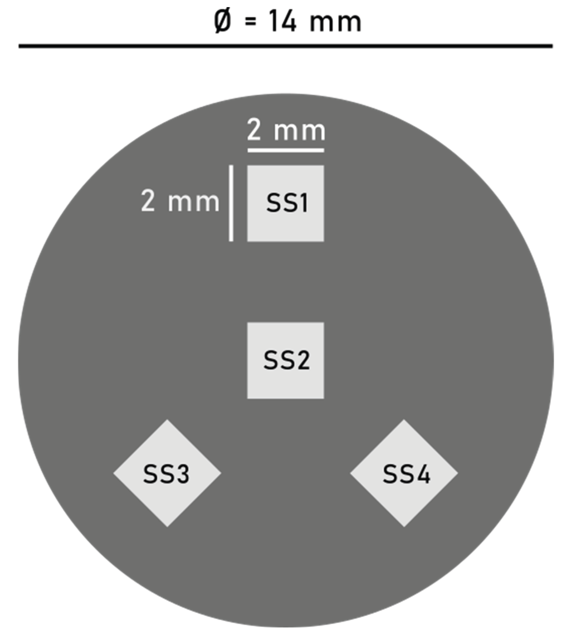
Figure 2.
Micrograph mosaic captured under darkfield illumination depicting sample B. ‘Mask’ refers to a masked version of the same image where all defined particles have been highlighted.
Figure 2.
Micrograph mosaic captured under darkfield illumination depicting sample B. ‘Mask’ refers to a masked version of the same image where all defined particles have been highlighted.
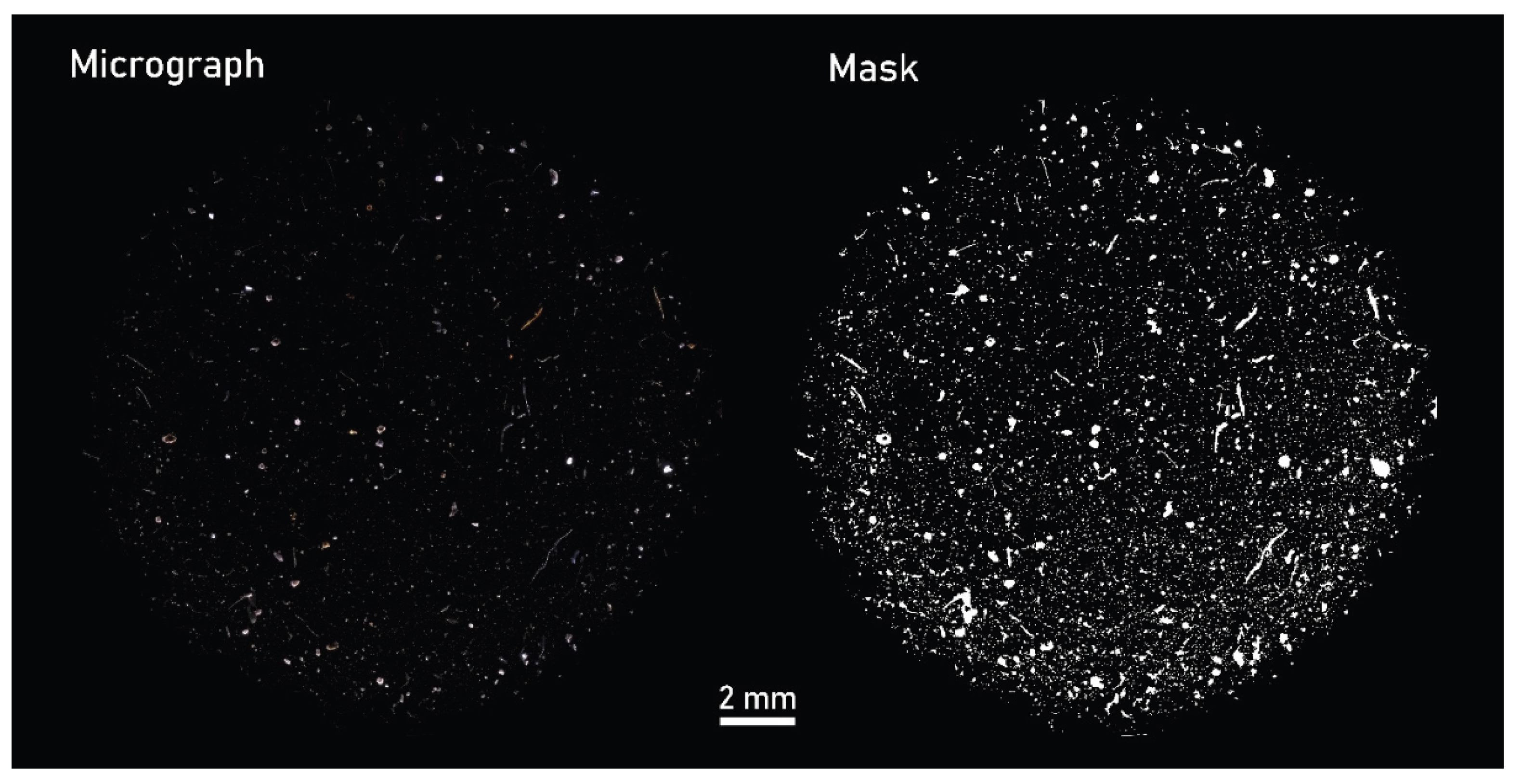
Figure 3.
Micrograph mosaic captured under darkfield illumination at a spatial resolution of 2.6 µm/pixel, depicting subsample 1 of sample 1. ‘Mask overlay’ uses distinct colors to define individual MP particles.
Figure 3.
Micrograph mosaic captured under darkfield illumination at a spatial resolution of 2.6 µm/pixel, depicting subsample 1 of sample 1. ‘Mask overlay’ uses distinct colors to define individual MP particles.
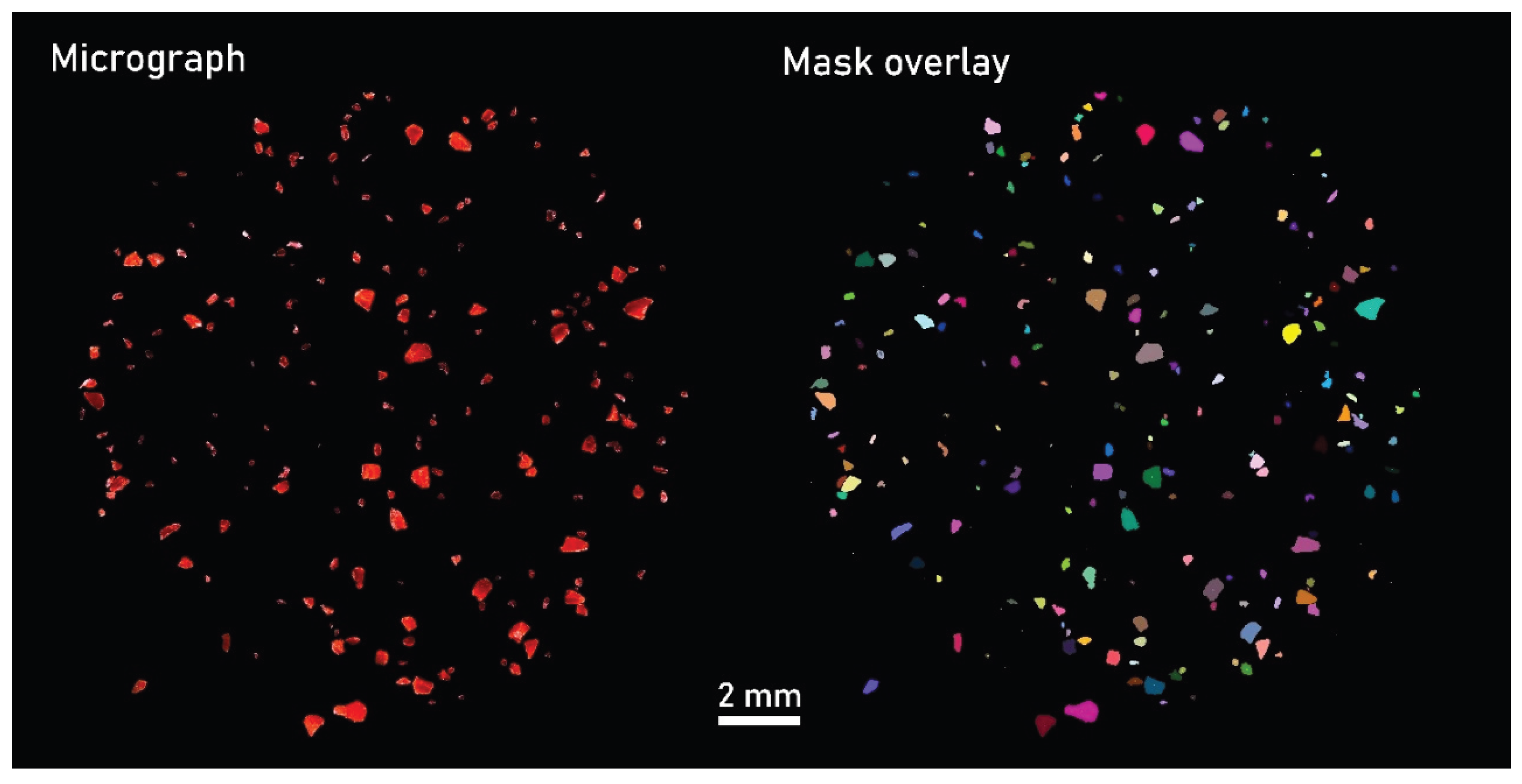
Figure 4.
Outlining of 2D particle morphology to volume conversion model (Hagelskjær model). A) Determine minimum Feret diameter (FMin). B) The height (h) of the particle is determined as FMin multiplied by the height multiplier Mh. C) The volume (V) of the particle is determined as H multiplied by the surface area (A) of the particle. Graphic made with Inkscape.
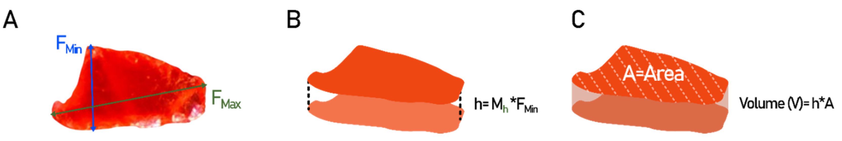
Figure 5.
Relative polymer type distribution (left) and particle size distribution (PSD) (right) of detected MPs between FOVs 1-4 of sample-A.
Figure 5.
Relative polymer type distribution (left) and particle size distribution (PSD) (right) of detected MPs between FOVs 1-4 of sample-A.
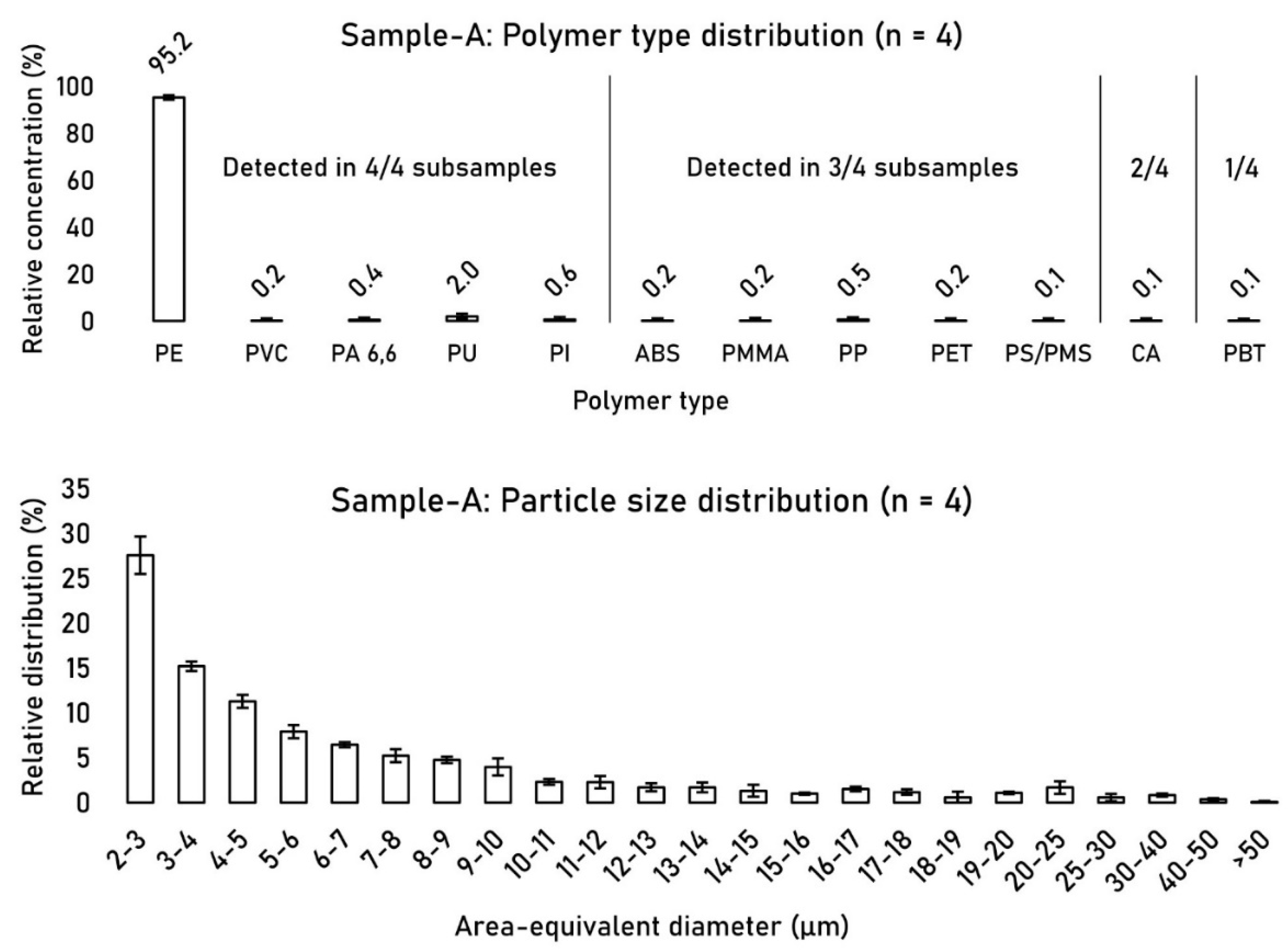
Figure 6.
Relative polymer type distribution (left) and particle size distribution (PSD) (right) of detected MPs between FOVs 1-4 of sample-B.
Figure 6.
Relative polymer type distribution (left) and particle size distribution (PSD) (right) of detected MPs between FOVs 1-4 of sample-B.
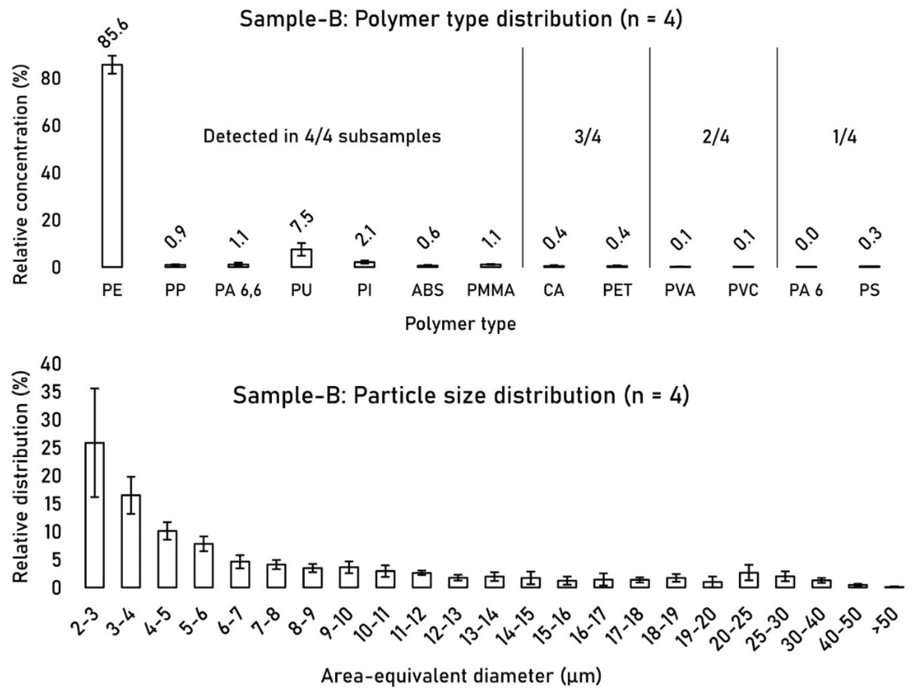
Figure 7.
Micrograph mosaics captured under darkfield illumination of subsamples 1-4 from samples 1-5 (20 subsamples total), showing MP fragments spanning 10 µm to 1500 µm (1.5 mm) in diameter.
Figure 7.
Micrograph mosaics captured under darkfield illumination of subsamples 1-4 from samples 1-5 (20 subsamples total), showing MP fragments spanning 10 µm to 1500 µm (1.5 mm) in diameter.
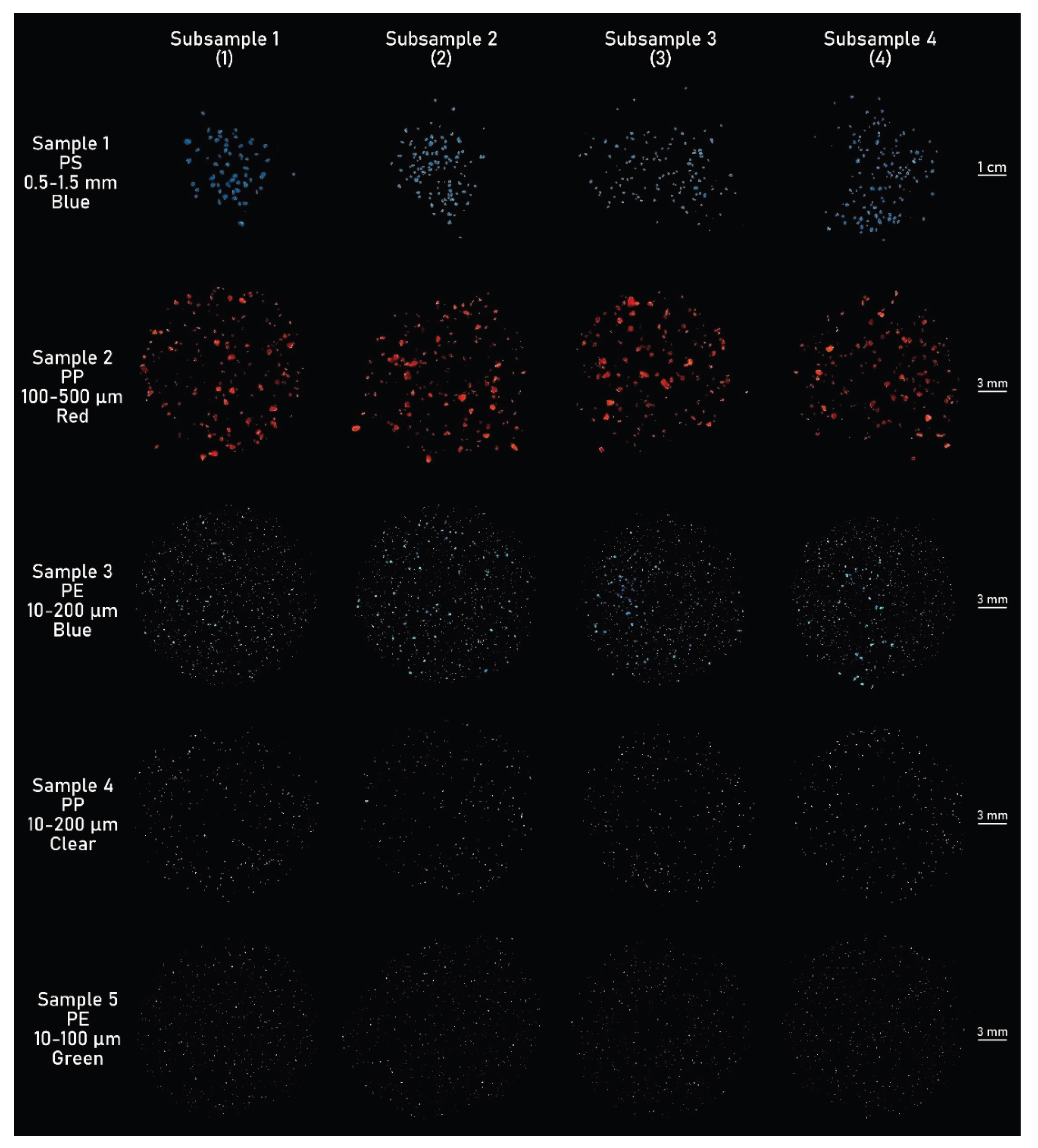
Figure 8.
Height multiplier (Mh) calibration results for subsamples 1-4 from samples 1-5 (n = 20). Sample identification: 1(2) denotes subsample 2 of sample 1. The solid black line represents the mean Mh (0.34), and the grey bar indicates ± the standard deviation (0.05).
Figure 8.
Height multiplier (Mh) calibration results for subsamples 1-4 from samples 1-5 (n = 20). Sample identification: 1(2) denotes subsample 2 of sample 1. The solid black line represents the mean Mh (0.34), and the grey bar indicates ± the standard deviation (0.05).
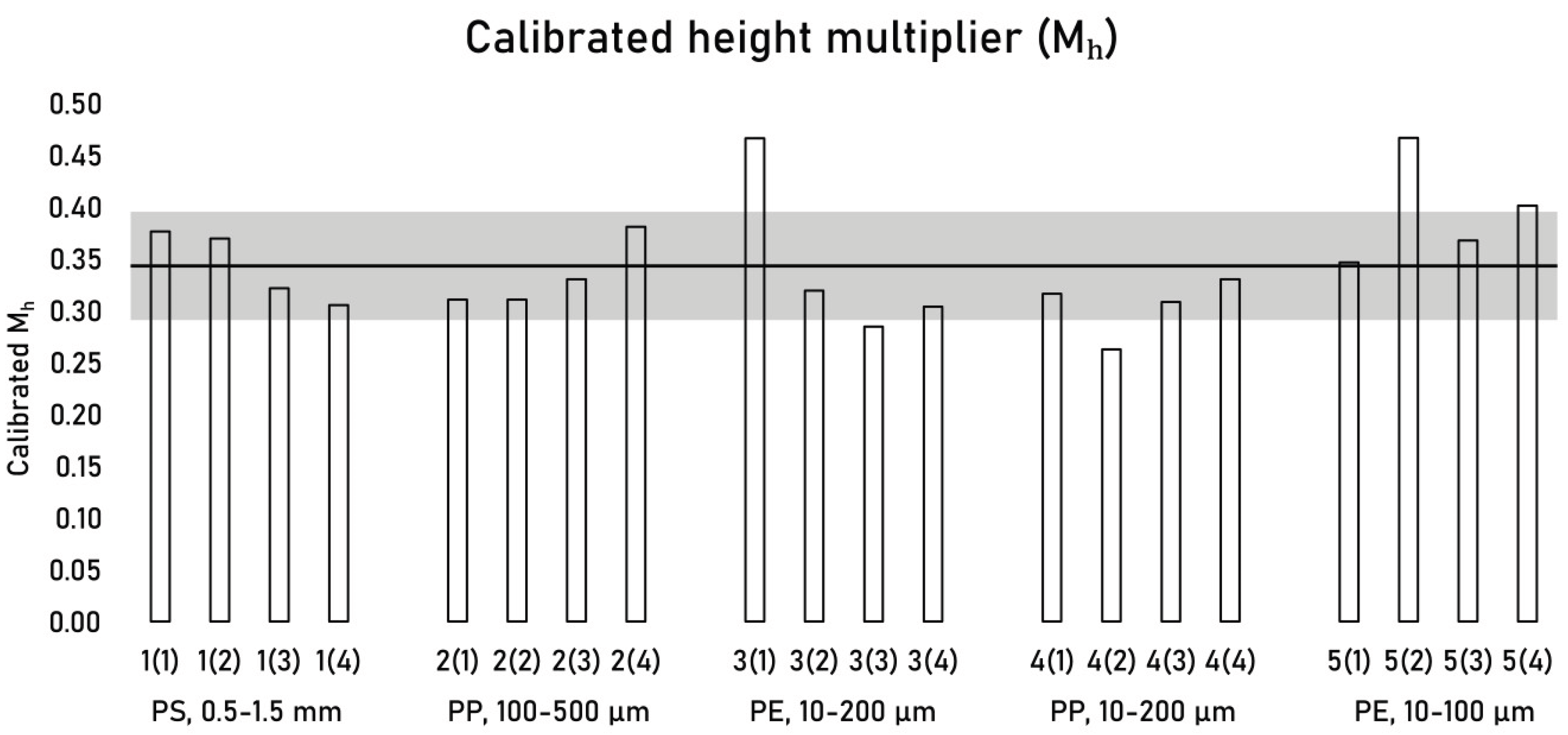
Figure 9.
Mean FMin/FMax ratios within individual subsamples. Sample identification: 1(2) denotes subsample 2 of sample 1. The error bars represent the standard deviation within the individual subsamples. The solid black line represents the mean FMin/FMax ratio (0.68), and the grey bar indicates ± the overall standard deviation (0.11).
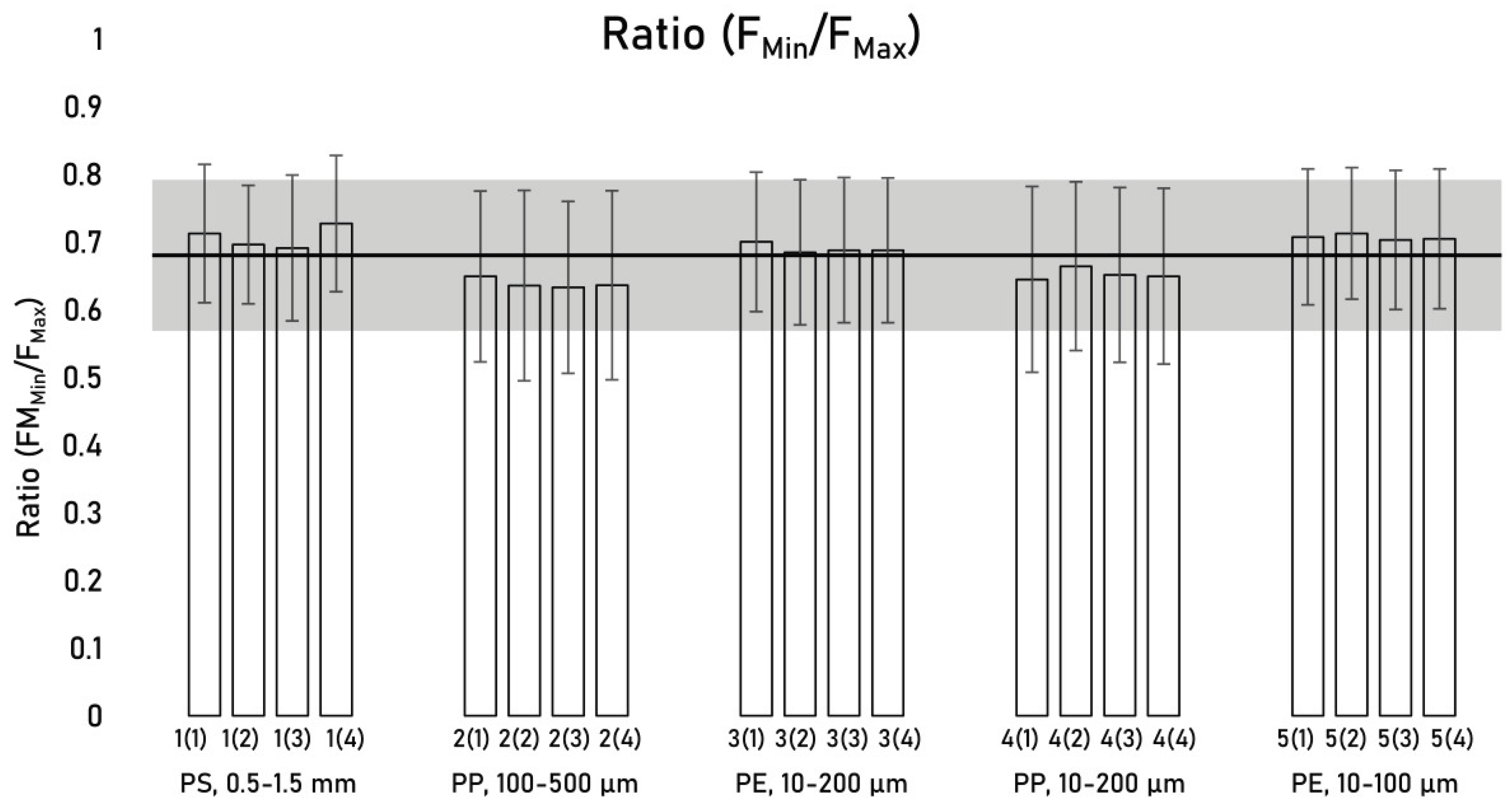

Table 1.
Particle count and surface area analysis for FOVs 1-4 of sample-A, showing generic particles, MP particles, area coverage ratios, and concentrations.
Table 1.
Particle count and surface area analysis for FOVs 1-4 of sample-A, showing generic particles, MP particles, area coverage ratios, and concentrations.
| Sample/Value | 1 (TOP) | 2 (LEFT) | 3 (RIGHT) | 4 (MID) | Mean | SD | RSD (%) |
|---|---|---|---|---|---|---|---|
| MP count (n) | 412 | 751 | 899 | 699 | 690 | 177 | 25.6 |
| Generic particle count (n) | 7087 | 16754 | 18850 | 20023 | 15679 | 5097 | 32.5 |
| MP count concentration (%) | 5.8 | 4.5 | 4.8 | 3.5 | 4.6 | 0.8 | 17.8 |
| MP area (µm²) | 2.77E+04 | 4.97E+04 | 7.68E+04 | 5.85E+04 | N/A | N/A | N/A |
| Generic particle area (µm²) | 2.43E+05 | 4.52E+05 | 6.42E+05 | 6.30E+05 | N/A | N/A | N/A |
| MPs (n) per generic particle area (µm²) | 0.0017 | 0.0017 | 0.0014 | 0.0011 | 0.0015 | 0.0002 | 16.0 |
| MP area concentration (%) | 11.4 | 11.0 | 12.0 | 9.3 | 10.9 | 1.0 | 9.1 |
| Particle area full filter (µm²) | 2.25E+07 | 2.25E+07 | 2.25E+07 | 2.25E+07 | N/A | N/A | N/A |
| Investigated particle area (%) | 1.08 | 2.01 | 2.85 | 2.80 | 2.2 | 0.72 | N/A |
Table 2.
Particle count and surface area analysis for FOVs 1-4 of sample-B, showing generic particles, MP particles, area coverage ratios, and concentrations.
Table 2.
Particle count and surface area analysis for FOVs 1-4 of sample-B, showing generic particles, MP particles, area coverage ratios, and concentrations.
| Sample/Value | 1 (TOP) | 2 (LEFT) | 3 (RIGHT) | 4 (MID) | Mean | SD | RSD (%) |
|---|---|---|---|---|---|---|---|
| MP count (n) | 620 | 364 | 403 | 302 | 422 | 120 | 28.4 |
| Generic particle count (n) | 23890 | 13616 | 23234 | 12662 | 18351 | 5228 | 28.5 |
| MP count concentration (%) | 2.6 | 2.7 | 1.7 | 2.4 | 2.3 | 0.4 | 15.7 |
| MP area (µm²) | 6.13E+04 | 3.08E+04 | 4.65E+04 | 1.19E+04 | N/A | N/A | N/A |
| Generic particle area (µm²) | 6.38E+05 | 3.40E+05 | 5.82E+05 | 4.77E+05 | N/A | N/A | N/A |
| MPs (n) per generic particle area (µm²) | 0.0010 | 0.0011 | 0.0007 | 0.0006 | 0.0008 | 0.0002 | 21.9 |
| MP area concentration (%) | 9.6 | 9.1 | 8.0 | 5.7 | 8.1 | 1.5 | 18.4 |
| Particle area full filter (µm²) | 2.04E+07 | 2.04E+07 | 2.04E+07 | 2.04E+07 | N/A | N/A | N/A |
| Investigated particle area (%) | 3.14 | 1.67 | 2.86 | 2.34 | 2.5 | 0.56 | N/A |
Table 3.
Summary data for investigated subsamples including weighed mass, calibrated height multiplier (Mh), number of MP particles, and particle size range. N/A = not applicable.
Table 3.
Summary data for investigated subsamples including weighed mass, calibrated height multiplier (Mh), number of MP particles, and particle size range. N/A = not applicable.
| Sample | Weighed Mass (µg) | Calibrated Height Multiplier (Mh) as per Eq. 2 | Number of Particles (n) | Size Range (µm) |
|---|---|---|---|---|
| 1(1) | 17400 | 0.376 | 57 | 500-1500 |
| 1(2) | 20400 | 0.369 | 102 | 500-1500 |
| 1(3) | 14000 | 0.321 | 118 | 500-1500 |
| 1(4) | 23400 | 0.305 | 133 | 500-1500 |
| 2(1) | 1042 | 0.311 | 207 | 100-500 |
| 2(2) | 1042 | 0.311 | 214 | 100-500 |
| 2(3) | 1042 | 0.330 | 193 | 100-500 |
| 2(4) | 1042 | 0.381 | 200 | 100-500 |
| 3(1) | 198 | 0.466 | 6344 | 10-200 |
| 3(2) | 198 | 0.319 | 5205 | 10-200 |
| 3(3) | 198 | 0.284 | 5246 | 10-200 |
| 3(4) | 198 | 0.304 | 5438 | 10-200 |
| 4(1) | 63.3 | 0.316 | 571 | 10-200 |
| 4(2) | 63.3 | 0.263 | 505 | 10-200 |
| 4(3) | 63.3 | 0.308 | 524 | 10-200 |
| 4(4) | 63.3 | 0.330 | 492 | 10-200 |
| 5(1) | 54 | 0.346 | 3140 | 10-100 |
| 5(2) | 54 | 0.466 | 3179 | 10-100 |
| 5(3) | 54 | 0.368 | 2740 | 10-100 |
| 5(4) | 54 | 0.401 | 3172 | 10-100 |
| Mean | N/A | 0.344 | N/A | N/A |
| SD | N/A | 0.053 | N/A | N/A |
| RSD (%) | N/A | 15.4 | N/A | N/A |
Disclaimer/Publisher’s Note: The statements, opinions and data contained in all publications are solely those of the individual author(s) and contributor(s) and not of MDPI and/or the editor(s). MDPI and/or the editor(s) disclaim responsibility for any injury to people or property resulting from any ideas, methods, instructions or products referred to in the content. |
© 2025 by the authors. Licensee MDPI, Basel, Switzerland. This article is an open access article distributed under the terms and conditions of the Creative Commons Attribution (CC BY) license (http://creativecommons.org/licenses/by/4.0/).
Copyright: This open access article is published under a Creative Commons CC BY 4.0 license, which permit the free download, distribution, and reuse, provided that the author and preprint are cited in any reuse.


