
Submitted:
14 July 2025
Posted:
16 July 2025
You are already at the latest version
Abstract
This paper introduces a novel probability distribution, the \textit{Half Logistic New Weibull-Pareto (HLNWP)} distribution, derived by applying a half logistic transformation to the New Weibull-Pareto family. The proposed distribution generalizes several existing models and offers enhanced flexibility in modeling diverse data behaviors. We derive and discuss key statistical properties including the probability density function, cumulative distribution function, hazard and reverse hazard functions, quantile function, moments, moment generating function, probability weighted moments, and order statistics. The maximum likelihood estimation (MLE) method is employed for parameter estimation, and analytical expressions for the score vector are provided. A comprehensive Monte Carlo simulation study is conducted to assess the performance and consistency of the MLEs. Finally, real-world data sets are analyzed to illustrate the applicability and superiority of the HL-NWP model in comparison with other non-nested alternatives. The results demonstrate the robustness and adaptability of the HL-NWP distribution for practical data modeling scenarios.
Keywords:
HLNWP distribution
; lifetime modeling
; reliability analysis
; hazard function
; maximum likelihood estimation
; simulation study
1. Introduction
Statistical models play a crucial role in research and data analysis as they help researchers to make inferences and predictions about the population from a sample [1]. One of the most important applications of statistical models is in modeling hazard rates of different types of data. Different statistical models have been developed to model hazard rates of data with varying complexities. The half logistic distribution proposed by [2], the generalized half logistic distribution first introduced by [3] where they introduced a class of distributions called the generalized exponential distributions which included the generalized half logistic distribution as a special case, the Weibull-Pareto distribution introduced by [4] as a member of beta-generated class of distributions, and the exponentiated half logistic-generalized G (EHL-GG) family of distributions [5] are just some few examples of statistical models used to model hazard rates.
The half logistic distribution originally proposed by [2] and its extensions such as the generalized half logistic distribution, Kumaraswamy half logistic distribution introduced by [6], Weibull-Pareto distribution [4], and EHL-GG family of distributions, have found wide applications in various fields for modeling data with monotonic and non-monotonic hazard rates, heavy-tailed data, and data with varying hazard rates. Despite their popularity, these distributions have limitations and may not always provide a good fit to all types of data [7]. Further research is needed to develop more flexible models that can better capture the complexity of real-world data. The half logistic distribution has been applied in different fields including rainfall data modeling [8], flood data modeling [9], and water flow modeling [10]. It has found extensive applications in modeling data that exhibit monotonic hazard rates. However, this distribution has limitations in modeling data with non-monotonic hazard rates, leading to the proposal of extensions such as the generalized half logistic distribution which applies to heavy tailed data and data that exhibit non-monotonic hazard rates.
Recently, [11] developed the New Weibull-Pareto (NWP) distribution and used it to model data with varying hazard rates, including data with constant, monotonic decreasing, and monotonic increasing hazard rate functions. The NWP distribution has been found to provide better fits to certain types of data compared to other commonly used distributions, gaining popularity in fields such as engineering, finance, and healthcare. The NWP distribution has found applications in wind speed data modeling [12], failure time modeling of electronic devices [13], and COVID-19 patient survival time modeling [14]. Moreover, the NWP distribution has also been employed in studies related to hydrology, finance, environmental science, and engineering [15]. [16] used the NWP distribution to model extreme precipitation events in the Yangtze River Basin, while [17] applied it to estimate value-at-risk in financial risk management. In another study, [18] used the NWP distribution to model the distribution of extreme daily rainfall in the Andean region. These studies highlight the wide range of applications of the NWP distribution, indicating its potential as a versatile and powerful tool for data analysis in various fields. The New Weibull-Pareto distribution offers a good fit for datasets with heavy tails and complex shapes, but it may not be suitable for datasets with a finite upper bound. It may also struggle to capture the complexity of some datasets, leading to poor model fit.
The cumulative distribution function (cdf) and probability density function (pdf) of the New Weibull-Pareto are given respectively by
and
for
[5] developed the exponentiated half logistic-generalized-G (EHL-GG) family of distributions which is a generalization of the half logistic distribution that offers a wider range of flexibility in modeling hazard rates. The EHL-GG family of distributions has been applied in modeling failure data of electric power transmission systems [15], concrete strength [19], and rainfall data [20]. Its ability to model various shapes of hazard rates, including increasing, decreasing, bathtub, and unimodal hazard rates, makes it a useful tool for analyzing data with complex hazard functions. Furthermore, the EHL-GG family is very flexible and can be used to model both continuous and discrete data, making it even more versatile for a wide range of applications. The cdf and pdf of the EHL-GG family of distributions are given respectively by
and
where is the baseline cdf with parameter vector , and are shape parameters. If we set , we obtain a half logistic-G (HL-G) generator with cdf given by
where is the baseline cdf with parameter vector , and .
The motivation for developing the Half Logistic-New Weibull-Pareto (HLNWP) distribution is the flexibility enjoyed after applying the HL-G transformation to models that exhibit monotonic hazard rate functions. The new distribution will possess both monotonic and non-monotonic hazard rate functions and applies to various levels of kurtosis and skewness, making it a useful model for data fitting and analysis in various fields.
2. The Half Logistic New Weibull Pareto Distribution
We use the half logistic-G generator given in (5) to transform the distribution given in (1) to come up with the Half Logistic New-Weibull Pareto (HLNWP) distribution with cdf and pdf given respectively by
and
for .
2.1. Sub-Models
We introduce some sub-models of the HLNWP distribution.
- When , we obtain the new Half Logistic Weibull (HLW) distribution with cdf and pdf given respectively byandfor ,
- When , we obtain the Half Logistic Exponential (HLE) distribution introduced by [21] with cdf and pdf given respectively byandfor .
- When and , we obtain the Half Logistic Rayleigh (HLR) distribution introduced by [22] with cdf and pdf given respectively asandfor .
- When , we obtain the Half Logistic Pareto (HLP) distribution, introduced by [23] with cdf and pdf given respectively asandfor .
3. Expansion of the Density Function
In this section we present an expansion of the density function. Rewriting the pdf of the HLNWP distribution in (7) we obtain
Using the series expansion
we have
Hence the pdf in (12) can be re-written as
which is a linear combination of the New Weibull Pareto distribution with power parameter , where is an exponentiated New-Weibull Pareto (NWP) distribution with power parameter .
The plots for the pdf of the HLNWP for different values of ,, and are given in Figure 1.
The density function reveals different shapes for various values of the parameters as shown in Figure 1. The plots show that the HLNWP distribution can handle data that display various shapes including reverse J, roughly symmetric, as well as data that is left or right-skewed.
4. Survival, Reverse Hazard and Hazard Functions
The survival function which gives the probability that a random variable X will take on a value larger than some specified value x, is defined as
where is the cdf. The survival function, reverse hazard function and the hazard function of the HLNWP distribution, are given respectively by
for , and .
The reverse hazard rate function, describes the probability of failure given survival time. In reliability analysis, the reverse hazard function provides information about the reliability of a system by modeling the probability that it will continue to function without failure beyond a certain time [24]. We thus have:
for , and .
We define the hazard function of the HLNWP distribution in terms of the density and survival functions as
where , and .
The plots for the hazard rate function (hrf) of the HLNWP for different values of are given in Figure 2.
The graph of the hazard function in Figure 2 exhibit increasing and unimodal shapes for selected values of the parameters. This flexibility makes the HLNWP hazard function useful and suitable for non-monotonic empirical hazard behaviours which are likely to be encountered in real life problems, and enables it to fit real lifetime datasets.
5. Quantile Function
In this section we derive the quantile function for the HLNWP distribution. The quantile function , defined by is the root of the equation, for We solve the following equation for
Thus, the quantile function is given as
Table 1 shows quantiles for selected values of , and of the HLNWP distribution.
6. Moments and Moment Generating Function
In this section we derive some statistical properties including the raw moments, the moment generating function, distribution of order statistics, as well as probability weighted moments for the HLNWP distribution.
6.1. Moments and Related Measures
In this section moments and related measures such as coefficient of variation, skewness and kurtosis of the HLNWP distribution are presented.
The moment, is given by
From the expanded pdf of the HLNWP distribution in (14), we have
Thus
Let then Also, When , and when , from (19) we have
The first four moments of the HLNWP distribution are given by
and
The mean (), variance( ), coefficient of variation (CV), coefficient of skewness (CS), and coefficient of kurtosis (CK) are given by
and
Table 2 lists the first five moments, standard deviation (SD), coefficient of variation (CV), coefficient of skewness (CS) and coefficient of kurtosis (CK) of the HLNWP distribution for some selected values of the parameters , and .
3-D Plots of skewness and kurtosis for selected fixed values of , and are presented in the figures below.
Figure 3.
Skewness and kurtosis plots for fixed values.
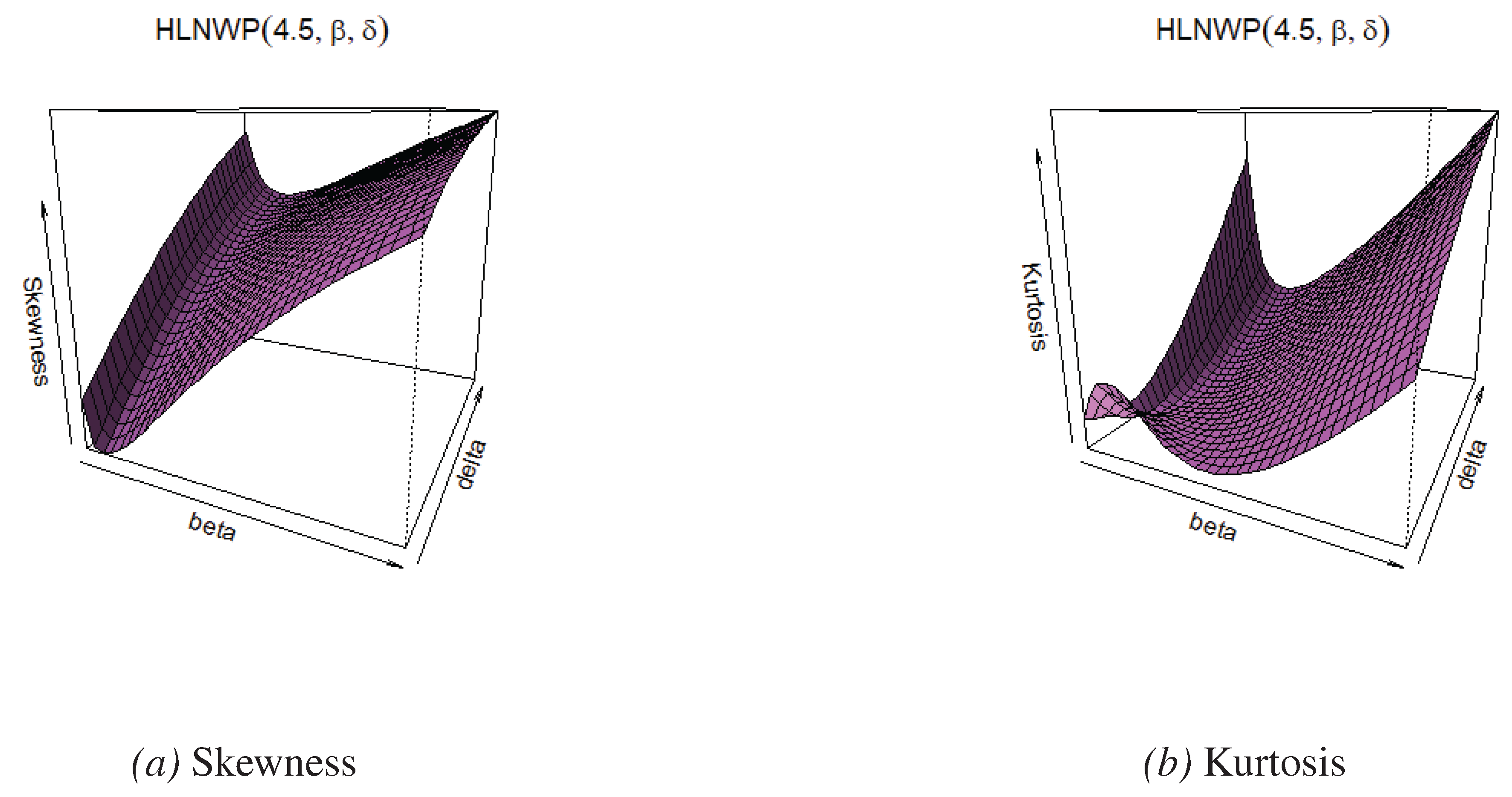
Figure 4.
Skewness and kurtosis plots for fixed values.
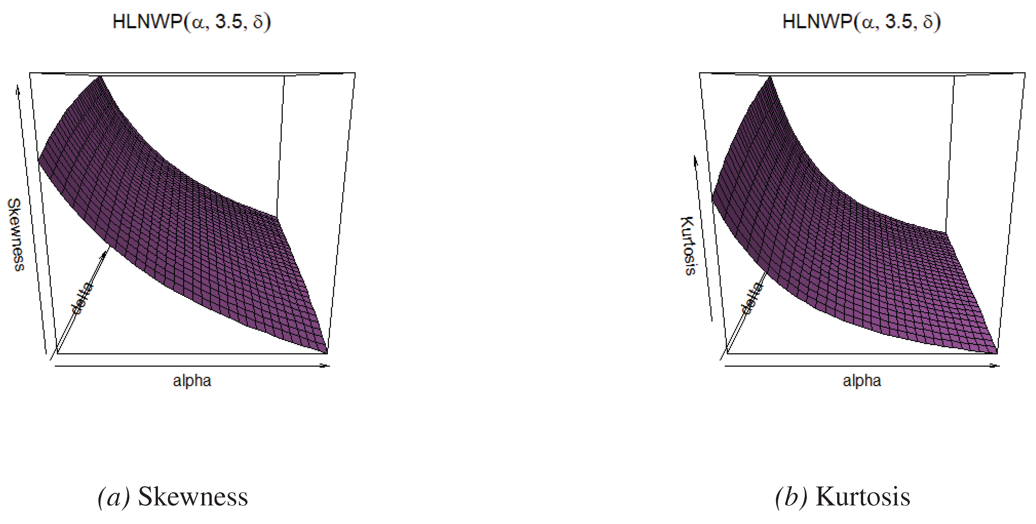
Figure 5.
Skewness and kurtosis plots for fixed values.
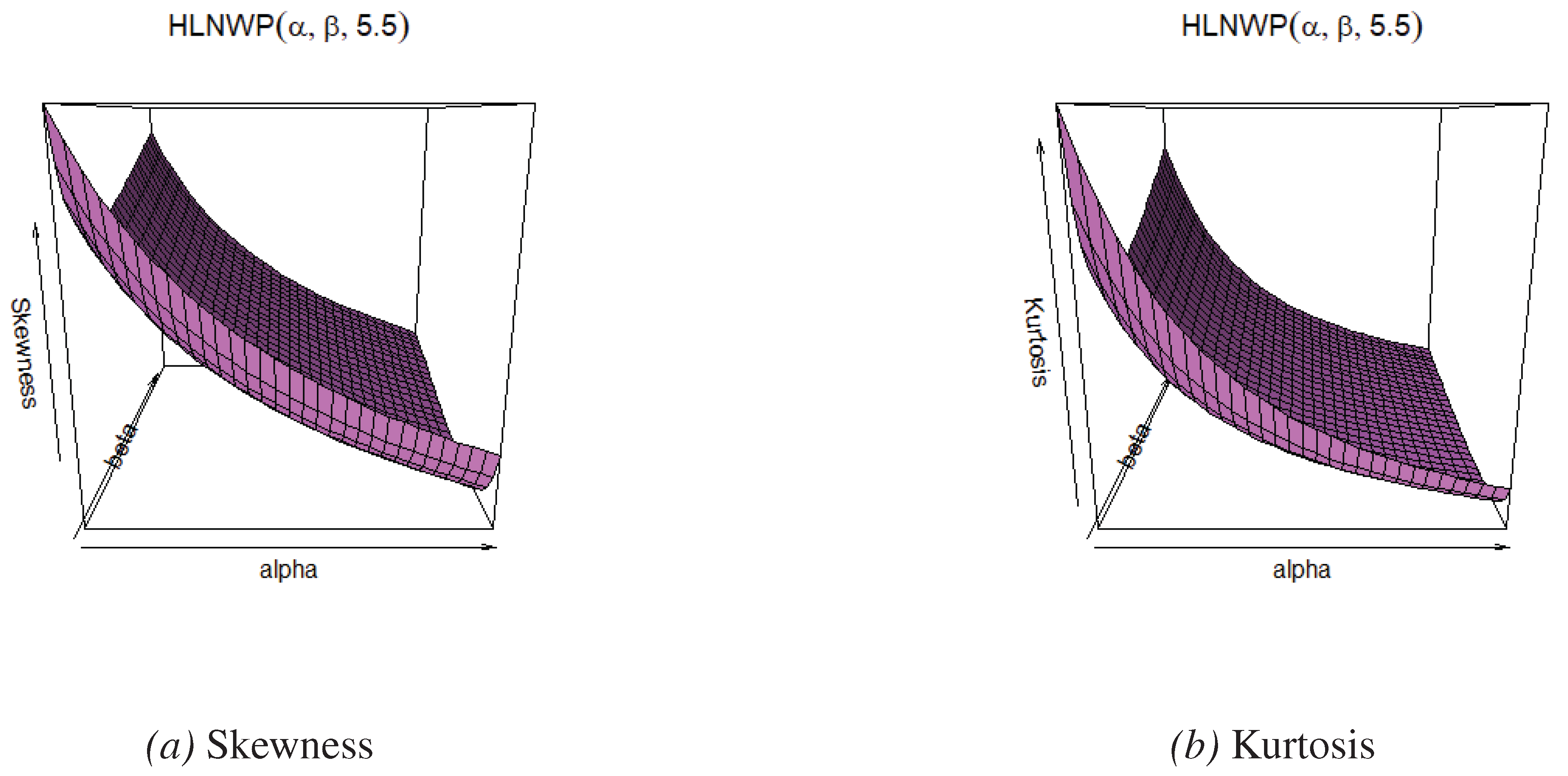
From these plots, we observe the following:
- When we fix the value of , skewness and kurtosis of the HLNWP distribution increase as the parameters and increase.
- When we fix the value of , skewness and kurtosis of the HLNWP distribution decrease as the parameters and increase.
- When we fix the value of , skewness and kurtosis of the HLNWP distribution decrease as the parameters and increase.
The moment generation function of the HLNWP is defined as
By the Taylor series expansion, we note that
Thus,
Using this result and substituting in (20), we have
6.2. Probability Weighted Moments
Probability weighted moments (PWMs) were introduced by [25] as a tool for estimating the parameters of a probability distribution. Unlike traditional moments, PWMs take into account the distribution of the data and weight each observation by its probability of occurrence. By incorporating the probability density function, PWMs can better capture the behavior of the underlying distribution and provide more accurate parameter estimates. The PWM for the HLNWP distribution is defined as
We have
Thus,
7. Distribution of Order Statistics
Let be a random sample from the HLNWP distribution and suppose that
denote the corresponding order statistics. The pdf of the order statistic is given by
where and are the cdf and pdf of HLNWP distribution given in (6) and (7) respectively. Using the series expansion
we can re-write (31) as
The Shannon entropy of the HLNWP distribution is defined as
We have
Note that for , using the series representation
Hence
Also,
Thus
Let
which implies
When , , and when , . From (38), we obtain
Using the moment given in (20) and substituting for the exponents, we obtain the expression for the Shannon entropy as
7.1. Rényi Entropy
Rényi entropy [26] is a generalization of Shannon entropy that includes a parameter that allows for tuning the level of sensitivity to rare events. Rényi entropy of the HLNWP distribution is defined as
Rényi entropy tends to Shannon entropy as . Using the pdf of the HLNWP given in (7) and the binomial identity given in (32) on the fourth term, we can express
Let
then
Also,
When , , and when , . From (40) we obtain
Thus,
8. Maximum Likelihood Estimation
In this section we use the method of maximum likelihood estimation to provide a basis for estimation of the parameters, and . We denote the parameter vector for the HLNWP distribution as .
The log-likelihood function of the HLNWP is:
The score function associated with the log-likelihood function is , where the first-order partial derivatives of the log-likelihood function are given by
and
The MLEs for can be obtained by solving the system . Solutions to the above equations are not in closed form, and so we opt for numerical methods such as optimization algorithms to obtain the estimates.
8.1. Fisher Information Matrix
The Fisher information matrix contains information that is useful for performing interval estimation and/or hypothesis testing. Under certain regularity conditions, the symmetric matrix that represents the Fisher information matrix (FIM) of the HLNWP distribution can be expressed as follows:
where the elements
The elements of the FIM can be obtained by considering the mixed second order partial derivatives of (42) with respect to the parameters and .
The mixed second order partial derivatives of (42) with respect to the parameters , and are given by
and
These elements can also be obtained numerically using R. We use the Fisher information to generate confidence intervals for the parameters of the HLNWP distribution.
9. Simulation Study
In this section an algorithm to generate random data from the HLNWP distribution is presented. A Monte-Carlo simulation study is also performed to evaluate the performance of the maximum likelihood estimators (MLE) for the parameters of the HLNWP distribution.
9.1. Generation Algorithm
We present an algorithm that we use to generate random data from the HLNWP distribution.
Algorithm:(Inverse Transform Sampling)
Let X be a random variable, where , with cdf
- 1.
- Generate Uniform (), .
- 2.
-
Set
9.2. Monte Carlo Simulation Study
In this section we study the performance of the HLNWP distribution by conducting various simulations for different combinations of 6 sample sizes with four sets of parameter values. The inverse transform sampling algorithm was used to generate random data from the HLNWP distribution. The simulation study was repeated times each with samples of sizes combined with parameter values , , , and . For the simulation, the value of was fixed to 1 as this parameter can be redundant and can be omitted without any loss to the meaning and performance of the simulation. The four quantities given below were computed in this simulation study.
- (a)
- Average bias of the MLE of the parameter
- (b)
- Root mean squared error (RMSE) of the MLE of the parameter
- (c)
- Coverage probability (CP) of 95% confidence intervals of the parameter , i.e., the percentage of intervals that contain the true value of parameter .
- (d)
- Average width (AW) of 95% confidence intervals of the parameter .
Table 3 and Table 4 display the Average Bias, Root Mean Square Error (RMSE), Coverage Probability (CP) and Average Width (AW) values of the parameters and for different sample sizes. The findings suggest that, as the sample size n increases, the RMSEs of the parameters decrease towards zero. Furthermore, for all parameters, the biases decrease as the sample size n increases. The results also indicate that the coverage probabilities of the confidence intervals are very close to the expected level of , and the average confidence interval widths decrease with larger sample sizes. Therefore, the Maximum Likelihood Estimates (MLEs) and their asymptotic results can be employed to estimate and construct confidence intervals even for relatively small sample sizes.
10. Applications
In this section we present examples to illustrate the flexibility and superiority of the HLNWP distribution in modeling real data. We compare the HLNWP distribution against some non-nested models, including the New Weibull Pareto (NWP) distribution [11], the Marshall-Olkin Log-logistic (MOLL) distribution introduced by [27], and the Marshall-Olkin Exponentiated Inverse Weibull (MOEIW) distribution introduced by [28]. The HLNWP distribution is also compared against its sub-models introduced in section 2. The density functions of the NWP, MOLL, and MOEIW distributions are respectively given by
for ,
for , ,
and
for ,
For each dataset, the estimates of the parameters of the distributions with their standard errors (in parentheses) are obtained by the method of maximum likelihood estimation. Some goodness of fit statistics including the Akaike Information Criterion (AIC) by [29], Consistent Akaike Information Criterion (CAIC) by [30], Bayesian Information Criterion (BIC) by [31], Cramer von Mises () [32], Anderson-Darling [33], the measure of closeness given by the sum of squares (SS) and Kolmogorov-Smirnov [34] (KS) test P-value are obtained. The model with the lowest AIC is generally considered the best fit for a particular dataset. When selecting a model based on the SS value, the model with the smallest SS is considered as the best fit model. When using the (KS) test P-value, the model with the highest P-value is considered the best among all others.
11. Covid-19 New Jersey Data
The dataset below as was reported in a study by [35] indicating the daily new deaths due to COVID-19 in New Jersey, USA, from March 12, 2020 to July 25, 2021. The dataset consists of the 201 observations as listed in Table 5.
The initial parameter values for the HLNWP distribution used for this dataset are ,
and . The results obtained for fitting the covid-19 New Jersey dataset are presented below. Estimates of the parameters of the distribution and their standard errors (in parentheses) are presented in Table 6. Some goodness of fit statistics including the -2logL, AIC, CAIC, BIC, , , SS and Kolmogorov-Smirnov (KS) test P-value are presented in in Table 7. These goodness of fit statistics will be used to compare the HLNWP to nested and other non-nested models.
We use the likelihood-ratio test to compare the goodness of fit between the HLNWP model against the nested models. That includes the HLW, HLE, HLR and HLP distributions.
To compare the HLW to the HLNWP model, we test the hypothesis
The test statistic
Thus we fail to reject the null hypothesis. At the significance level, we can similarly conclude that the HLW distribution provides a good fit to the covid-19 New Jersey dataset in as much as the HLNWP distribution. Again, this supports the conclusion made earlier that could be a redundant parameter for the non-nested HLNWP model.
Similarly, to compare the HLE to the HLNWP model, we test the hypothesis
The test statistic
Thus we reject the null hypothesis. At the significance level we can assert that the HLNWP provides a better fit for this dataset than the HLE nested model.
Comparing the HLR to the HLNWP model, we test the hypothesis
The test statistic
Thus we reject the null hypothesis. At the significance level we can assert that the HLNWP provides a better fit for this dataset than the HLR nested model.
Comparing the HLP to the HLNWP model, we test the hypothesis
The test statistic
Thus we reject the null hypothesis. At the significance level we can assert that the HLNWP provides a better fit for this dataset than the HLP nested model.
We also conclude that the HLNWP distribution also provides a better fit for the covid-19 New Jersey dataset than the non-nested NWP, MOLL, and MOEIW distributions as it has a lower value of AIC, CAIC, BIC, SS and a higher value of the KS test P-Value, presented in Table 7.
The asymptotic covariance matrix of the MLEs of the HLNWP model parameters for the covid-19 New Jersey dataset, is given by
The confidence intervals for the model parameters , and are given respectively by
All the estimates are significant as the intervals do not include 0.
We have shown in Table 7 that the HLNWP fits the covid-19 New Jersey dataset better than the other models compared to it. Plots of the fitted densities of the highlighted distributions imposed on the histogram of the covid-19 New Jersey data is shown in Figure 6. Figure 7 shows a plot of the empirical cdf (ecdf) against the theoretical cdf and we observe that the line representing the theoretical values match up well with the empirical values. Figure 8 shows probability plots of the highlighted distributions on this dataset, and we observe that the HLNWP model fits better with a relatively lower SS value compared to the other distributions. The plots in Figure 9 and Figure 10 reiterate the fact that the HLNWP provides a good fit for this data, as the lines representing theoretical values, match up well with fitted data. Figure 11 shows that the model applies to a monotonically increasing hazard rate for this dataset.
12. Kevlar70 Data
The Kevlar70 dataset below represents observations of tensile strength measurements for modeling the tensile strength of Kevlar fibers [36]. The dataset consists of the 49 observations as listed in Table 8.
The initial parameter values for the HLNWP distribution used for this dataset are ,
and . The results obtained for fitting the Kevlar70 dataset are presented below. Estimates of the parameters of the distribution and their standard errors (in parentheses) are presented in Table 9. Some goodness of fit statistics including the -2logL, AIC, CAIC, BIC, , , SS and Kolmogorov-Smirnov (KS) test P-value are presented in in Table 10. These goodness of fit statistics will be used to compare the HLNWP to nested and other non-nested models.
Similarly, we use the likelihood-ratio test to compare the goodness of fit between the HLNWP model against the nested models. This includes the HLW, HLE, HLR and HLP distributions.
To compare the HLW to the HLNWP model, we test the hypothesis
The test statistic
Thus we fail to reject the null hypothesis. At the significance level, we can conclude that the HLW distribution provides a good fit to the Kevlar70 dataset. However, based on the higher KS P-value, and a lower SS value of the HLNWP distribution outlined in Table 10, we can conclude that the HLNWP model provides a better fit for this dataset than the HLW distribution.
Similarly, to compare the HLE to the HLNWP model, we test the hypothesis
The test statistic
Thus we reject the null hypothesis. At the significance level we can assert that the HLNWP provides a better fit for the Kevlar70 dataset than the HLE nested model.
Comparing the HLR to the HLNWP model, we test the hypothesis
The test statistic
Thus we reject the null hypothesis. At the significance level we can assert that the HLNWP provides a better fit for this dataset than the HLR nested model.
Also, to compare the HLP to the HLNWP model, we test the hypothesis
The test statistic
Thus we reject the null hypothesis. At the significance level we can assert that the HLNWP provides a better fit for the Kevlar70 dataset than the HLP nested model.
We also conclude that the HLNWP distribution also provides a better fit for the Kevlar70 dataset than the non-nested NWP, MOLL, and MOEIW distributions as it has a lower value of AIC, CAIC, BIC, SS and a higher value of the KS test P-Value, presented in Table 10.
The asymptotic covariance matrix of the MLEs of the HLNWP model parameters for the Kevlar70 dataset, is given by
The confidence intervals for the model parameters , and are given respectively by
All the estimates are significant as the intervals do not include 0.
We have shown in Table 10 that the HLNWP fits the Kevlar70 dataset better than the other models compared to it. Plots of the fitted densities of the highlighted distributions imposed on the histogram of the Kevlar70 data is shown in Figure 12. Figure 13 shows a plot of the empirical cdf (ecdf) against the theoretical cdf and we observe that the line representing the theoretical values match up well with the empirical values. Figure 14 shows probability plots of the highlighted distributions on this dataset, and we observe that the HLNWP model fits better with a relatively lower SS value compared to the other distributions. The plots in Figure 15 and Figure 16 reiterate the fact that the HLNWP provides a good fit for this data, as the lines representing theoretical values, match up well with fitted data. Figure 17 shows that the model applies to a monotonically increasing hazard rate for this dataset.
Although the Half-Logistic Weibull (HLW) submodel exhibits lower values for the Akaike Information Criterion (AIC), Bayesian Information Criterion (BIC), and corrected AIC (AICc), indicating greater parsimony, the full HLNWP model provides a superior empirical fit based on the Kolmogorov–Smirnov (K–S) test. Specifically, the HLNWP model yields a higher K–S p-value, suggesting that it more accurately captures the underlying data distribution. This highlights a trade-off between model simplicity and goodness-of-fit, where the HLW model is more efficient in terms of parameter economy, while the HLNWP model better represents the observed data behavior.
13. Conclusions
We have proposed a new distribution that is a transformation of the New Weibull-Pareto distribution. The half logistic transformation was used in this research to develop the new distribution called Half Logistic-New Weibull-Pareto (HLNWP) distribution. We have shown that the HLNWP has a set of new nested models when we fix some of the parameters. These include the Half Logistic Weibull, Half Logistic Exponential, Half Logistic Rayleigh and the Half Logistic Pareto distributions. Statistical properties of the new model have been developed. These properties include hazard and reverse hazard functions, quantile function, raw moments, moment generating function, probability weighted moments, and distribution of order statistics. In addition to these properties, measures of uncertainty, and reliability for the HLNWP distribution have been obtained. The hazard function of the HLNWP distribution has different shapes including monotonically increasing and unimodal shapes.
Elements of the score vector for the maximum likelihood estimates of the model parameters have been derived. We have presented a simulation study to exhibit the performance of the HLNWP distribution. Real data applications have also been presented to illustrate the usefulness and applicability of the HLNWP distribution, and we have seen that this new model provides a better fit to the data than its nested models, and also the highlighted non-nested NWP, MOLL and the MOEIW models.
Acknowledgments
This preprint version is identical to the manuscript submitted for peer review, except for the inclusion of author names and affiliations for compliance with preprint server requirements. The manuscript is currently under peer review and has not been certified by a journal.
References
- Tong, C. Statistical inference enables bad science; statistical thinking enables good science. The American Statistician 2019, 73, 246–261.
- Balakrishnan, N. Order statistics from the half logistic distribution. Journal of statistical computation and simulation 1985, 20, 287–309.
- Gupta, R.; Kundu, D. Generalized exponential distributions. Australian & New Zealand Journal of Statistics 1999, 41, 173–188.
- Balakrishnan, N.; Kundu, D. A review of beta-generated distributions. Brazilian Journal of Probability and Statistics 2009, 23, 280–319.
- Cordeiro, G.M.; Alizadeh, M.; Ortega, E.M. The exponentiated half-logistic family of distributions: Properties and applications. Journal of Probability and Statistics 2014, 2014.
- Kundu, D.; Raqab, M.Z. A new class of Kumaraswamy-G family of distributions. Journal of King Saud University-Science 2016, 28, 190–199.
- Vayansky, I.; Kumar, S.A. A review of topic modeling methods. Information Systems 2020, 94, 101582.
- Das, S. On the use of half logistic distribution in rainfall data analysis. Journal of Hydrologic Engineering 2020, 25, 04020100.
- Javadi, H.; Malekmohammadi, B.; Ahmadi, M. Flood frequency analysis using the half logistic distribution. Water Resources Management 2019, 33, 1637–1650.
- Saravanan, S.; Srinivasan, S.; Anand, R. The half logistic distribution as an alternative to the log-normal distribution for water flow modeling. Journal of Hydrology 2020, 583, 124624.
- Nasiru, S.; Luguterah, A. The new weibull-pareto distribution. Pakistan Journal of Statistics and Operation Research 2015, pp. 103–114.
- Balakrishnan, N.; Lu, J. The Weibull-Pareto distribution for modeling wind speed data. Journal of Applied Statistics 2019, 46, 1361–1374.
- Qiu, X.; Wu, Y.; Ren, W. Weibull-Pareto distribution based on the failure time modeling of electronic devices. Journal of Applied Statistics 2021, pp. 1–20.
- Wei, J.; Chen, W.; Li, L.; Wang, J.; Yang, W.; Wu, X.; Zeng, G. Modeling survival time of COVID-19 patients using the Weibull-Pareto distribution. Journal of Clinical Medicine 2021, 10, 871.
- Balakrishnan, N. Exponentiated half logistic-generalized G family of distributions: properties and applications. Journal of Statistical Distributions and Applications 2018, 5, 1–24.
- Wang, D.; Zhang, Y.; Zhu, J.; He, Y. A Weibull-Pareto distribution model for extreme precipitation events in the Yangtze River Basin. Hydrological Sciences Journal 2019, 64, 611–622.
- Khan, M.S.; Rathore, V.S.; Chan, F.T. Estimating Value-at-Risk using Weibull-Pareto distribution: A new approach. Economic Modelling 2019, 82, 267–279.
- Navarro-Estupi n’an, J.; Mora-Rubio, V.; C’elleri, R. Extreme rainfall modeling in the Andean region using the Weibull-Pareto distribution. Water Resources Management 2019, 33, 3471–3486.
- Singh, R.K. Generalized half logistic generalized G family of distributions with application. Heliyon 2019, 5, e02599.
- Sharma, M. A new exponentiated half logistic generalized G family of distributions with applications. Journal of Statistical Theory and Practice 2020, 14, 1–17.
- Nadarajah, S.; Ahsanullah, M. A Half-Logistic Exponential Distribution. Communications in Statistics-Theory and Methods 2011, 40, 4025–4036.
- Al-Babtain, A.A. A new extended Rayleigh distribution. Journal of King Saud University-Science 2020, 32, 2576–2581.
- Nadarajah, S.; Ahsanullah, M. The half-logistic Pareto distribution and its applications. Journal of Probability and Statistics 2013, 2013.
- Birolini, A. Reliability Engineering: Theory and Practice; Springer International Publishing, 2015.
- Greenwood, J.A.; Landwehr, J.M.; Matalas, N.C.; Wallis, J.R. Probability weighted moments: definition and relation to parameters of several distributions expressable in inverse form. Water resources research 1979, 15, 1049–1054.
- Rényi, A. On measures of entropy and information. In Proceedings of the Proceedings of the Fourth Berkeley Symposium on Mathematical Statistics and Probability, Volume 1: Contributions to the Theory of Statistics. University of California Press, 1961, Vol. 4, pp. 547–562.
- Wenhao, G. Marshall-Olkin extended log-logistic distribution and its application in minification processes. Applied Mathematical Sciences 2013, 7, 3947–3961.
- Pakungwati, R.; Widyaningsih, Y.; Lestari, D. Marshall-Olkin extended inverse Weibull distribution and its application. In Proceedings of the Journal of physics: conference series. IOP Publishing, 2018, Vol. 1108, p. 012114.
- Akaike, H. A new look at the statistical model identification. IEEE transactions on automatic control 1974, 19, 716–723.
- Hurvich, C.M.; Tsai, C.L. Regression and time series model selection in small samples. Biometrika 1989, 76, 297–307.
- Schwarz, G. Estimating the dimension of a model. The annals of statistics 1978, pp. 461–464.
- Cramer, H. On the composition of elementary errors. Skand. Aktuarietidskr 1928, 11, 13–74.
- Anderson, T.W.; Darling, D.A. Asymptotic theory of certain “goodness-of-fit” criteria based on stochastic processes. The Annals of Mathematical Statistics 1952, 23, 193–212.
- Smirnov, N. Table for estimating the goodness of fit of empirical distributions. The Annals of Mathematical Statistics 1948, 19, 279–281.
- Muhammad, M.; Liu, L.; Abba, B.; Muhammad, I.; Bouchane, M.; Zhang, H.; Musa, S. A New Extension of the Topp–Leone-Family of Models with Applications to Real Data. Journal of Data Science 2021, 19, 747–769.
- Aggarwala, R.; Cook, R.D. Modeling the tensile strength of Kevlar fibers. Technometrics 2000, 42, 180–189.
Figure 1.
Plots of the probability density function for different values of , , and .
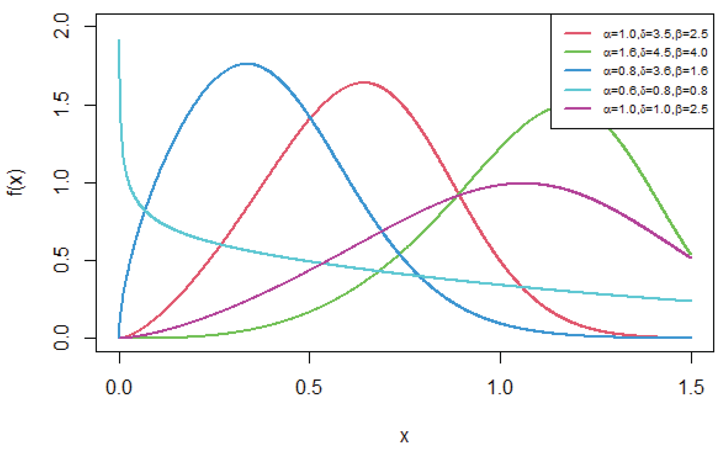
Figure 2.
Plots of the hazard rate function for different values of , and .
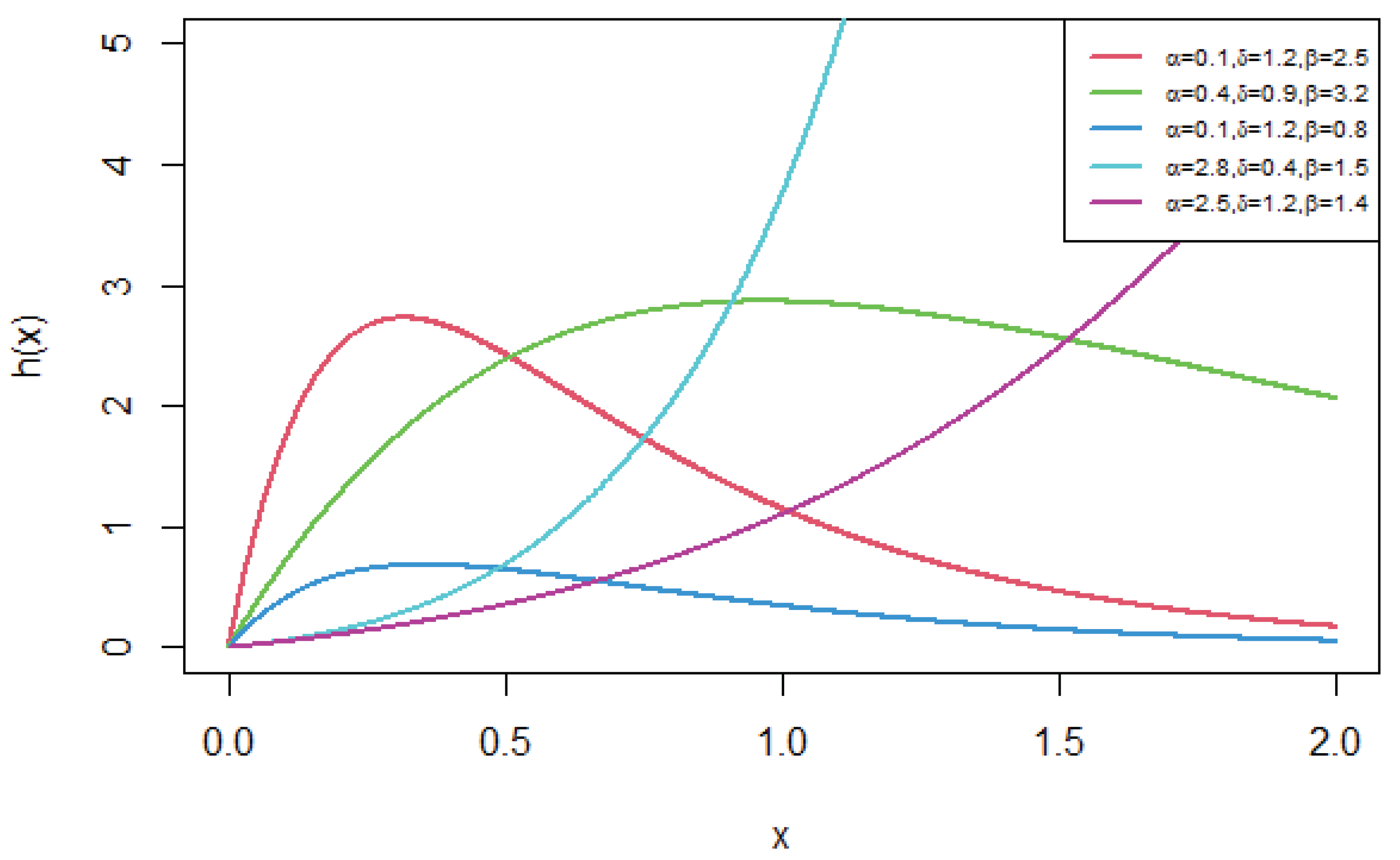
Figure 6.
Fitted PDFs for Covid-19 New Jersey Data
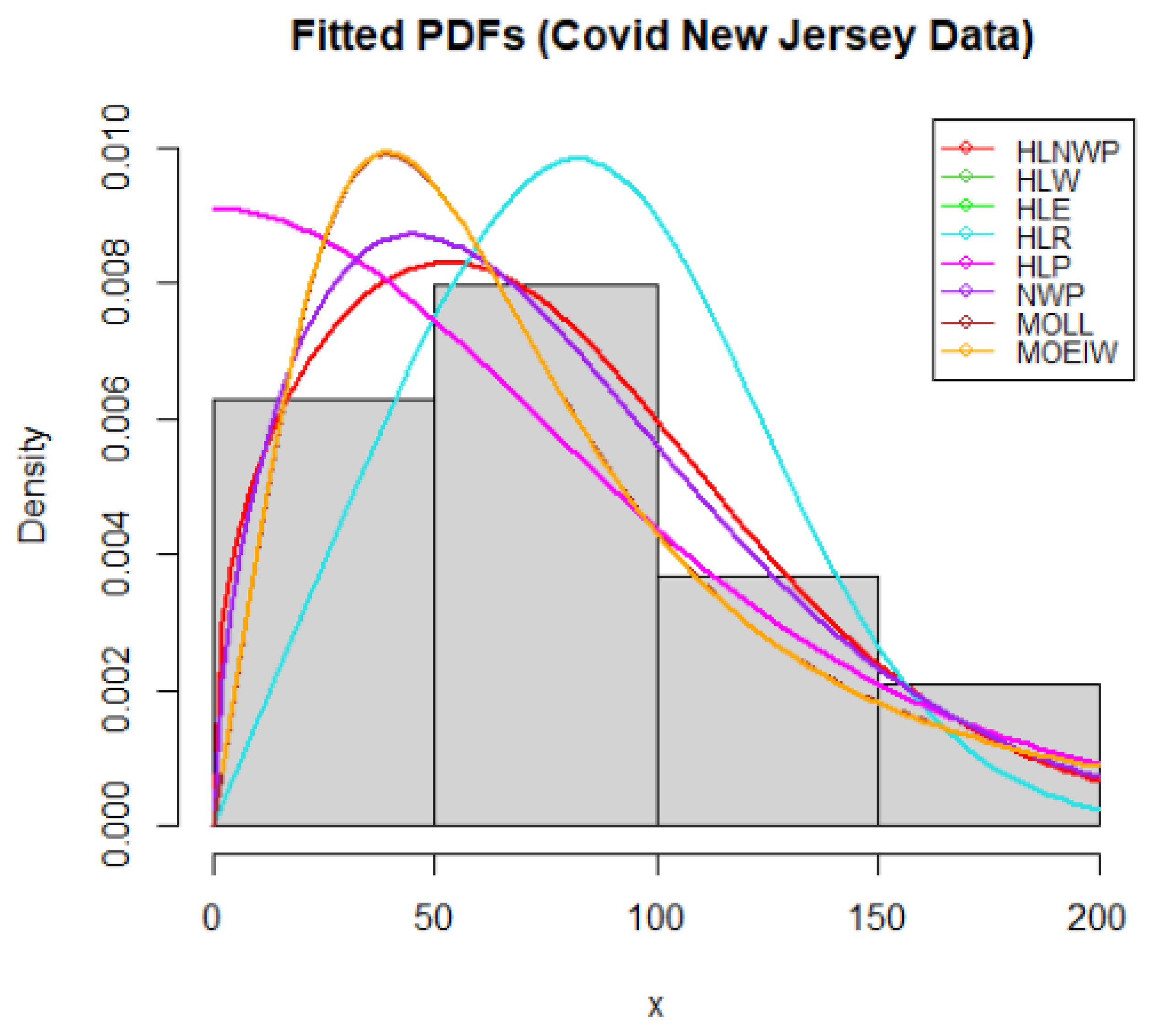
Figure 7.
Plot of Empirical cdf for Covid-19 New Jersey Data
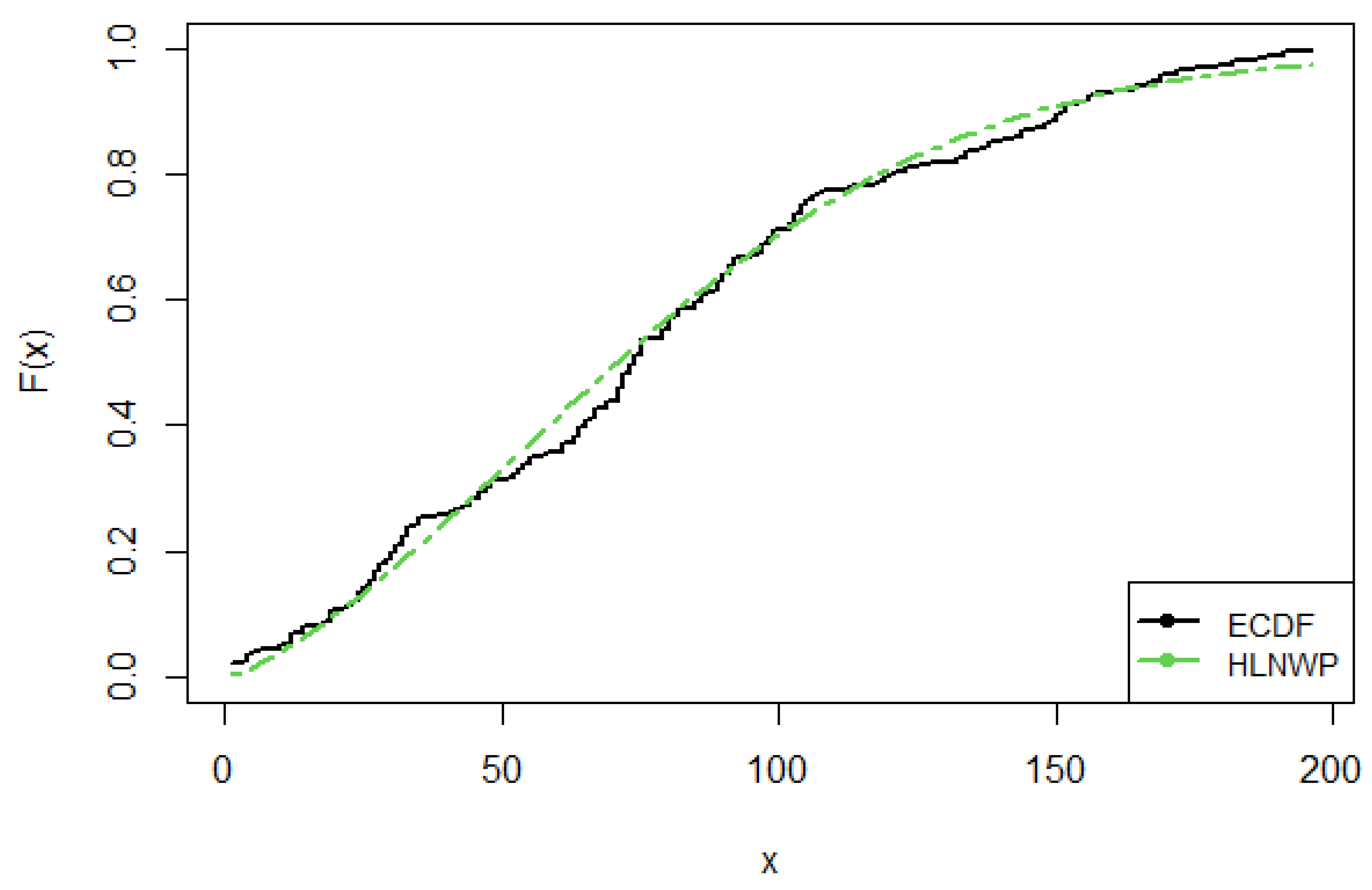
Figure 8.
Probability Plots for Covid-19 New Jersey Data
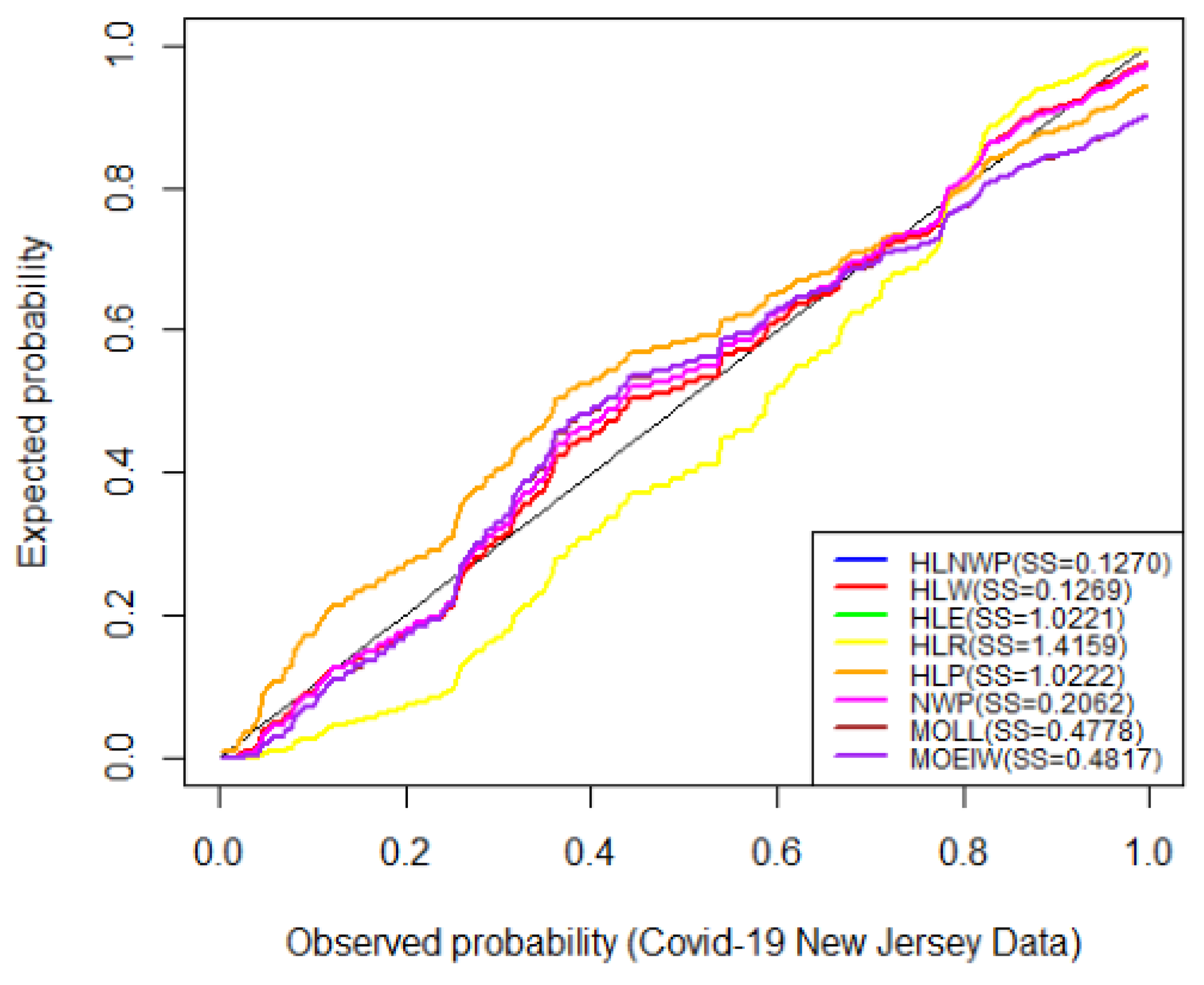
Figure 9.
KM Plot for Covid-19 New Jersey Data
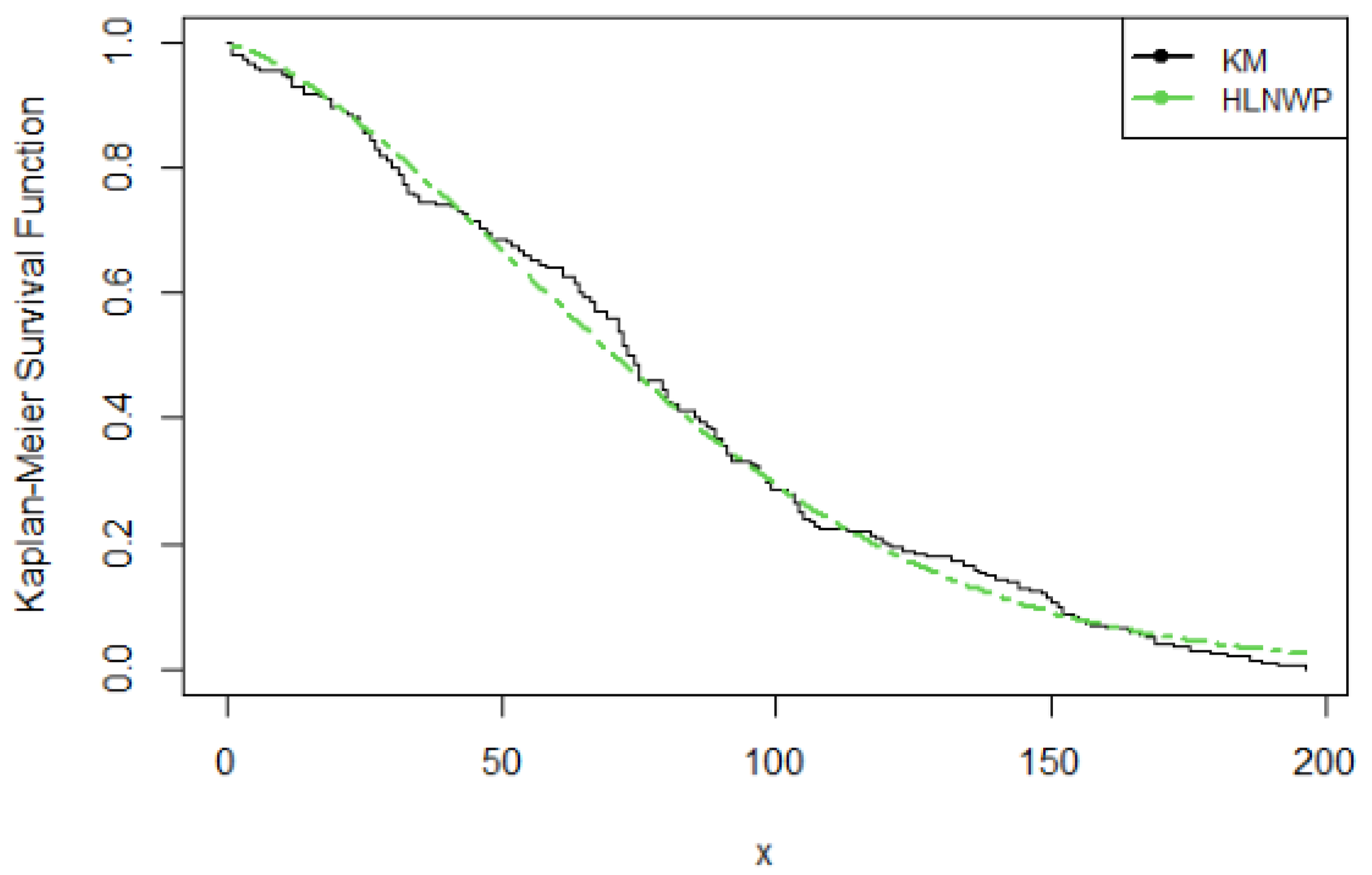
Figure 10.
Scaled TTT-Transform Plot for Covid-19 New Jersey Data
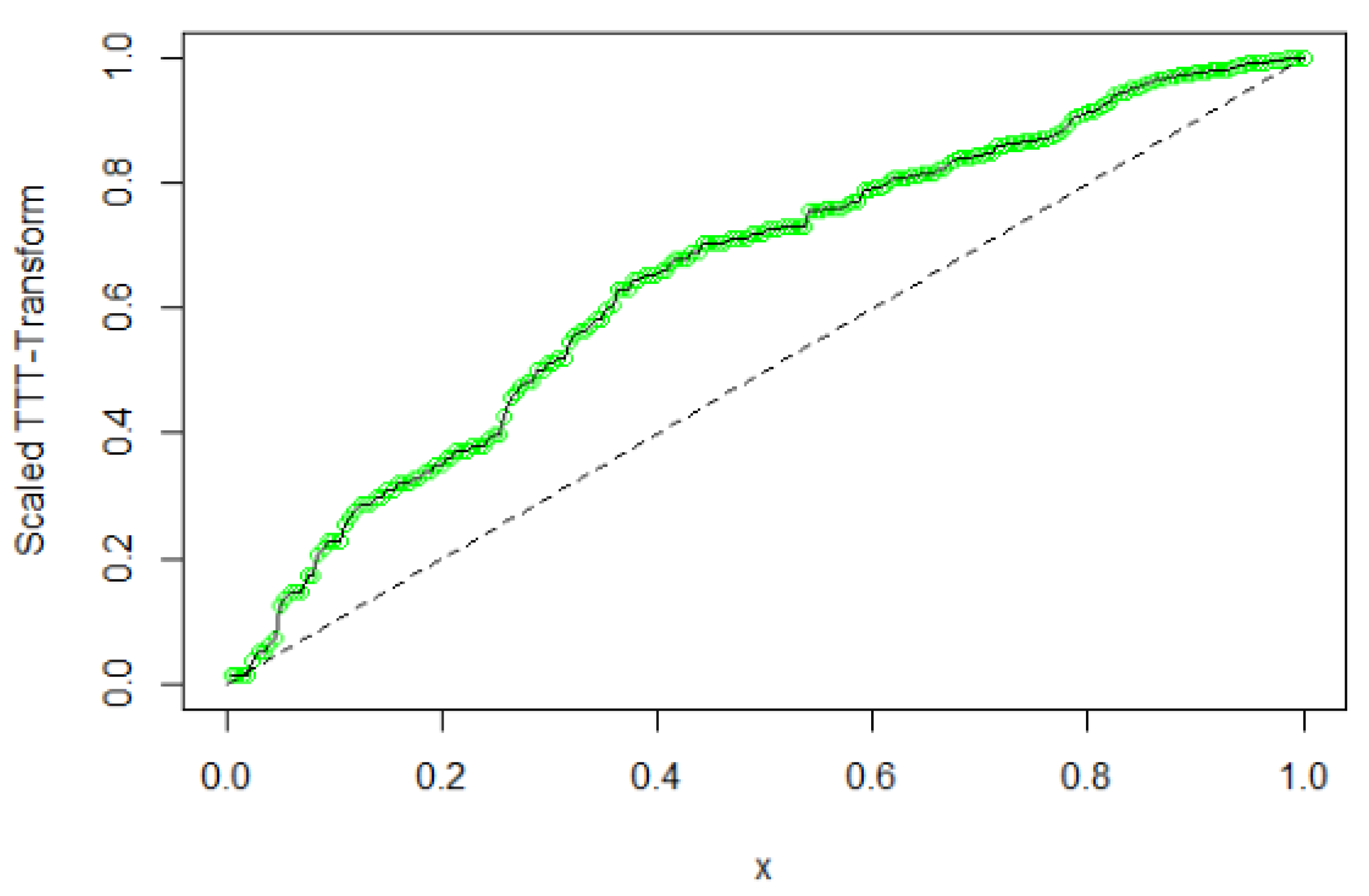
Figure 11.
Fitted hrf Plot for Covid-19 New Jersey Data
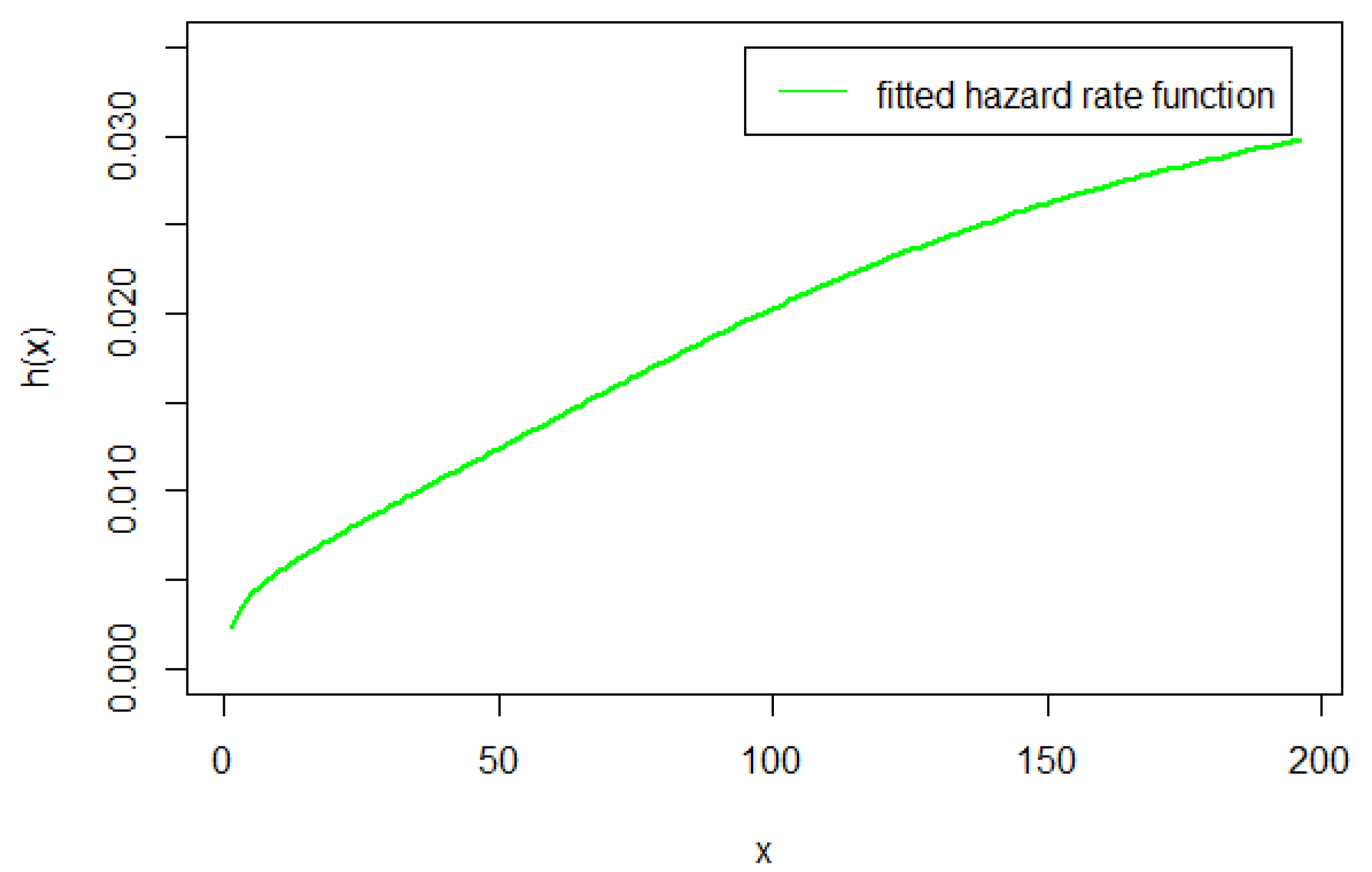
Figure 12.
Fitted PDFs for Kevlar70 Data
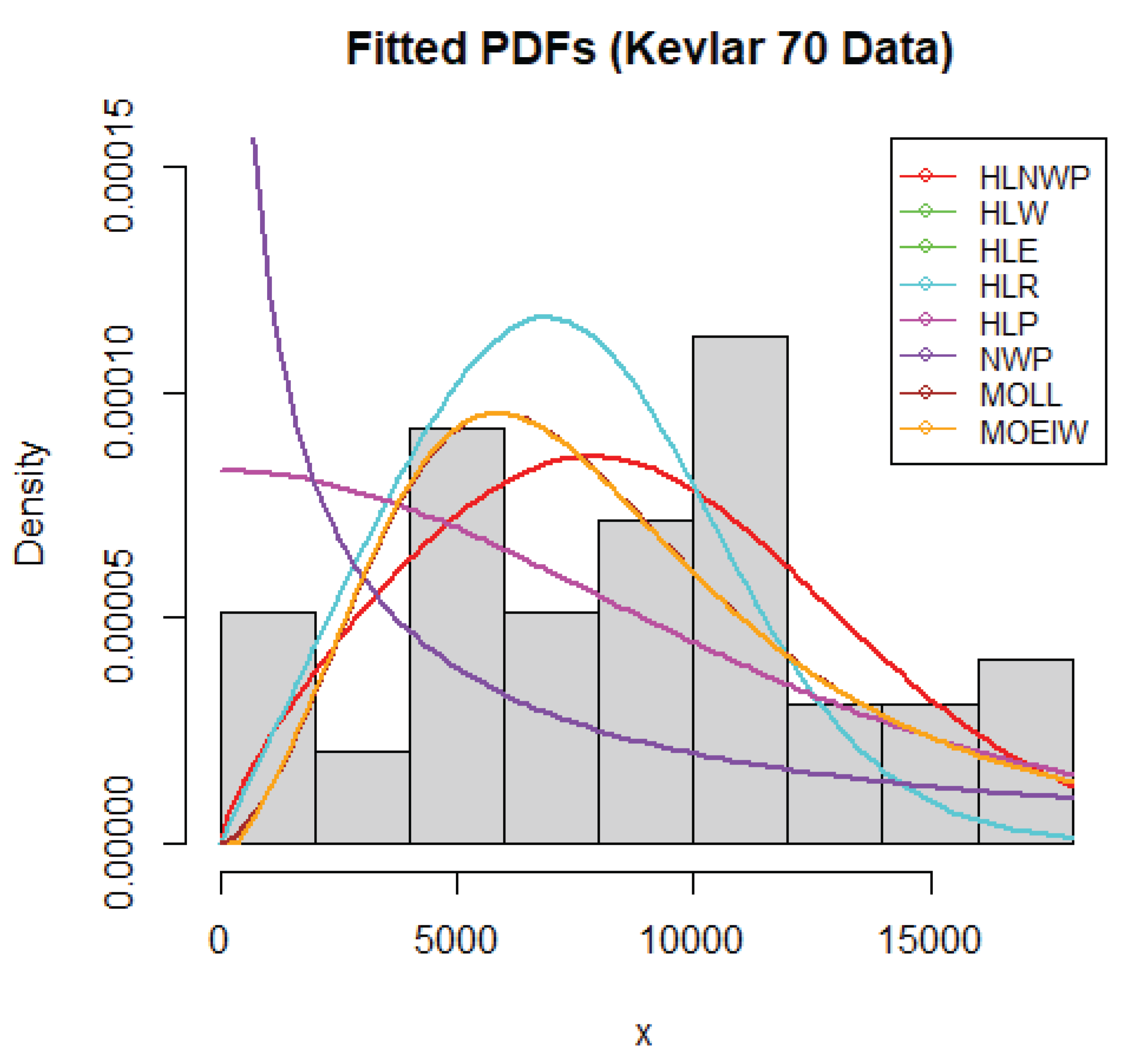
Figure 13.
Plot of Empirical cdf for Kevlar70 Data
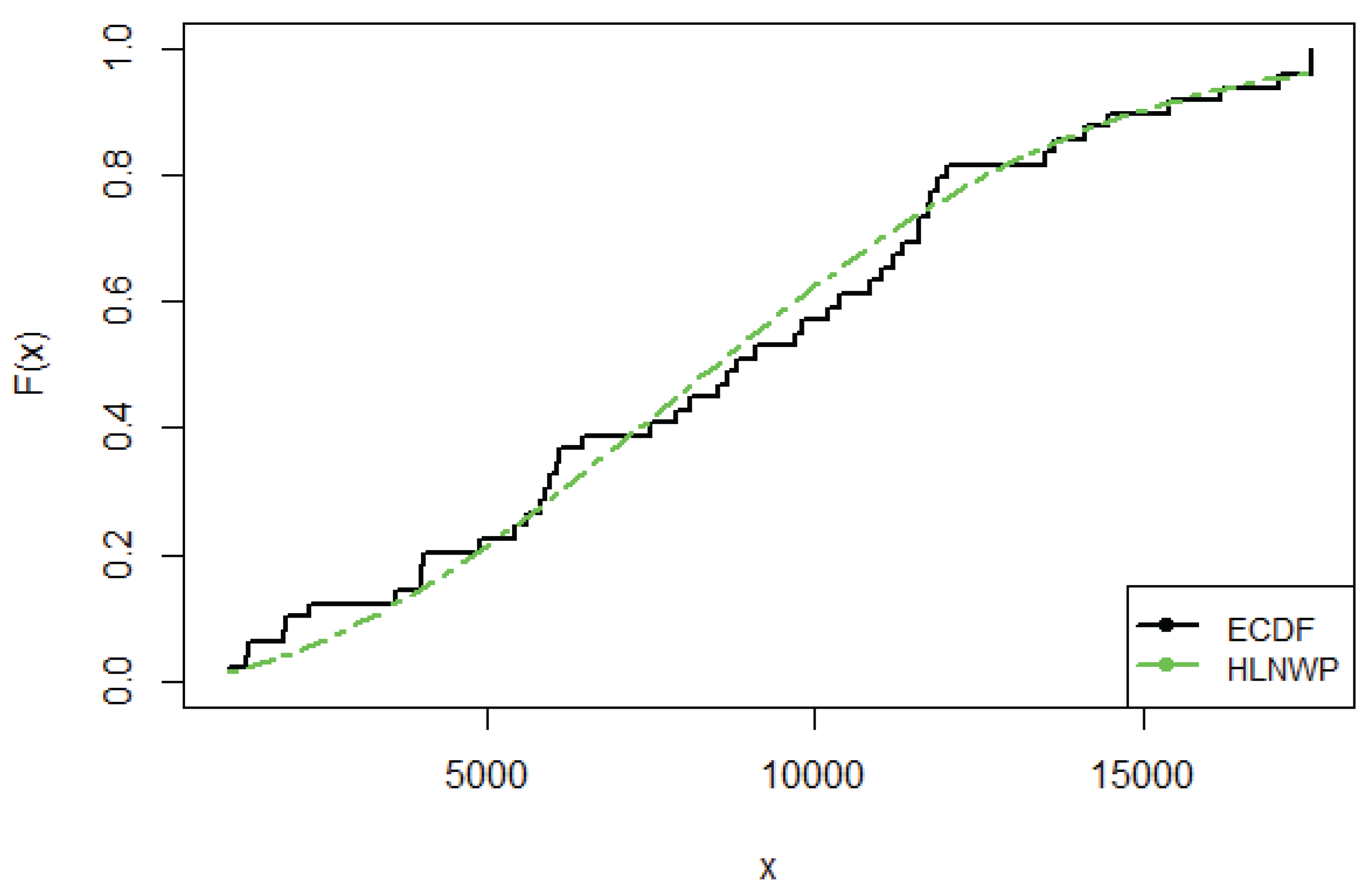
Figure 14.
Probability Plots for Kevlar70 Data
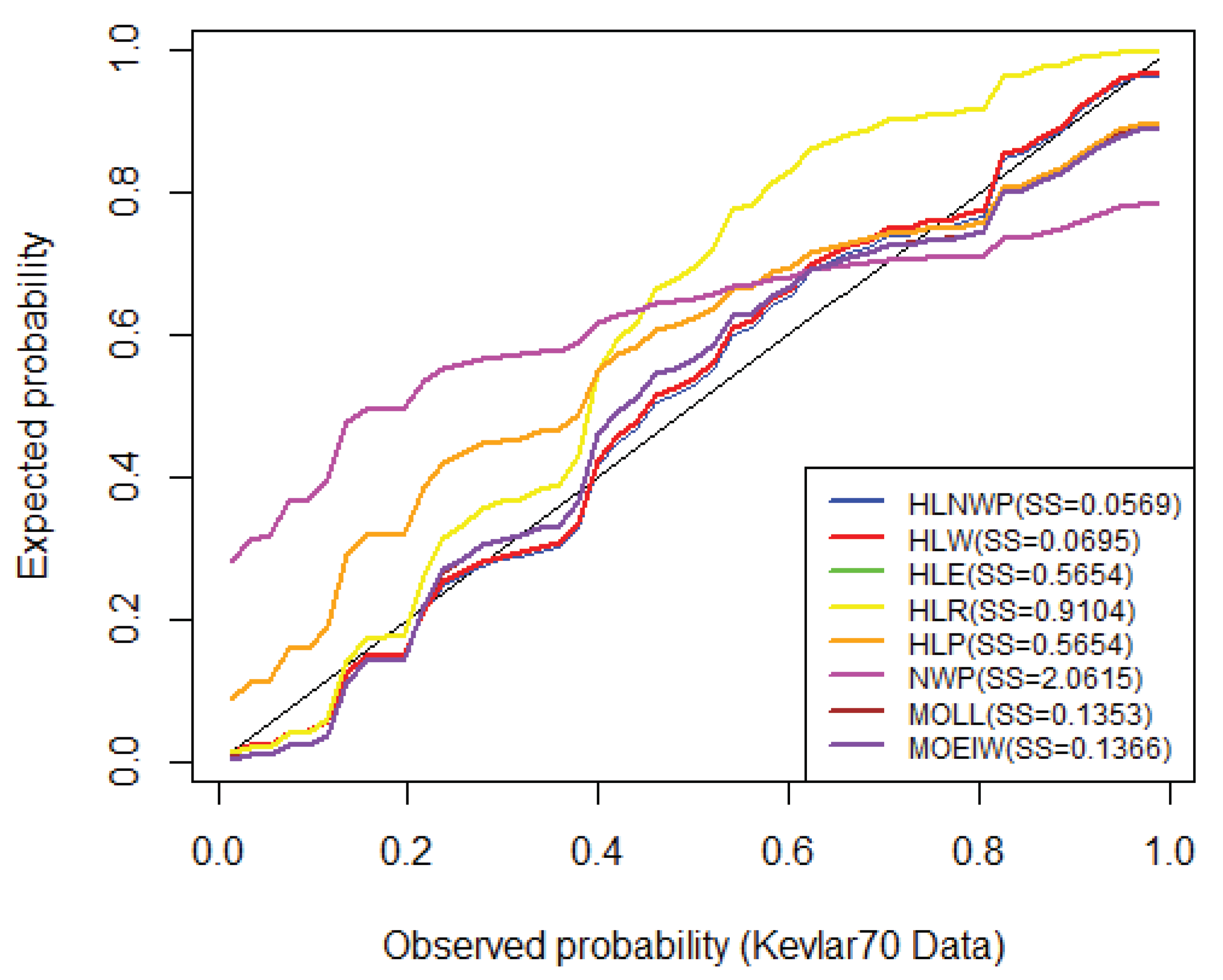
Figure 15.
KM Plot for Kevlar70 Data
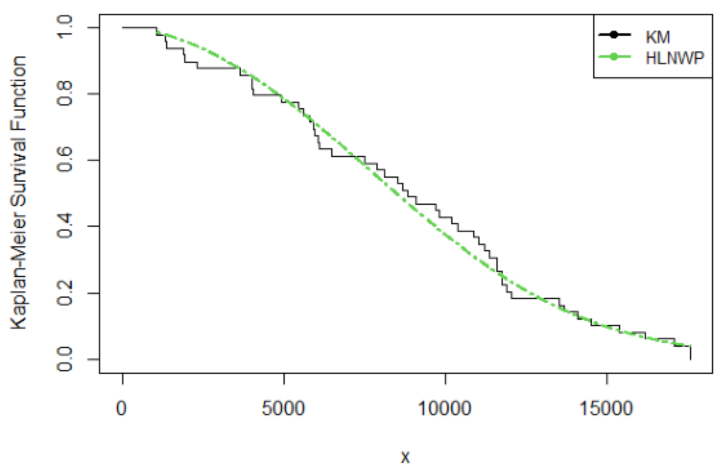
Figure 16.
Scaled TTT-Transform Plot for Kevlar70 Data
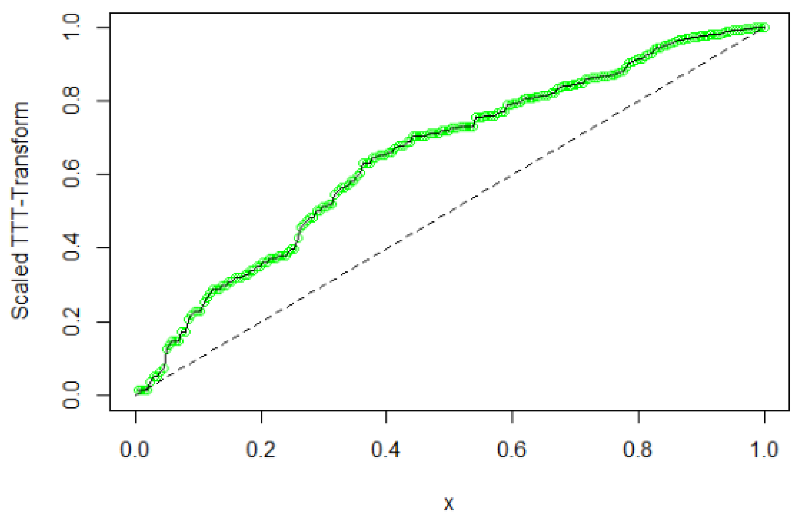
Figure 17.
Fitted hrf Plot for Kevlar70 Data
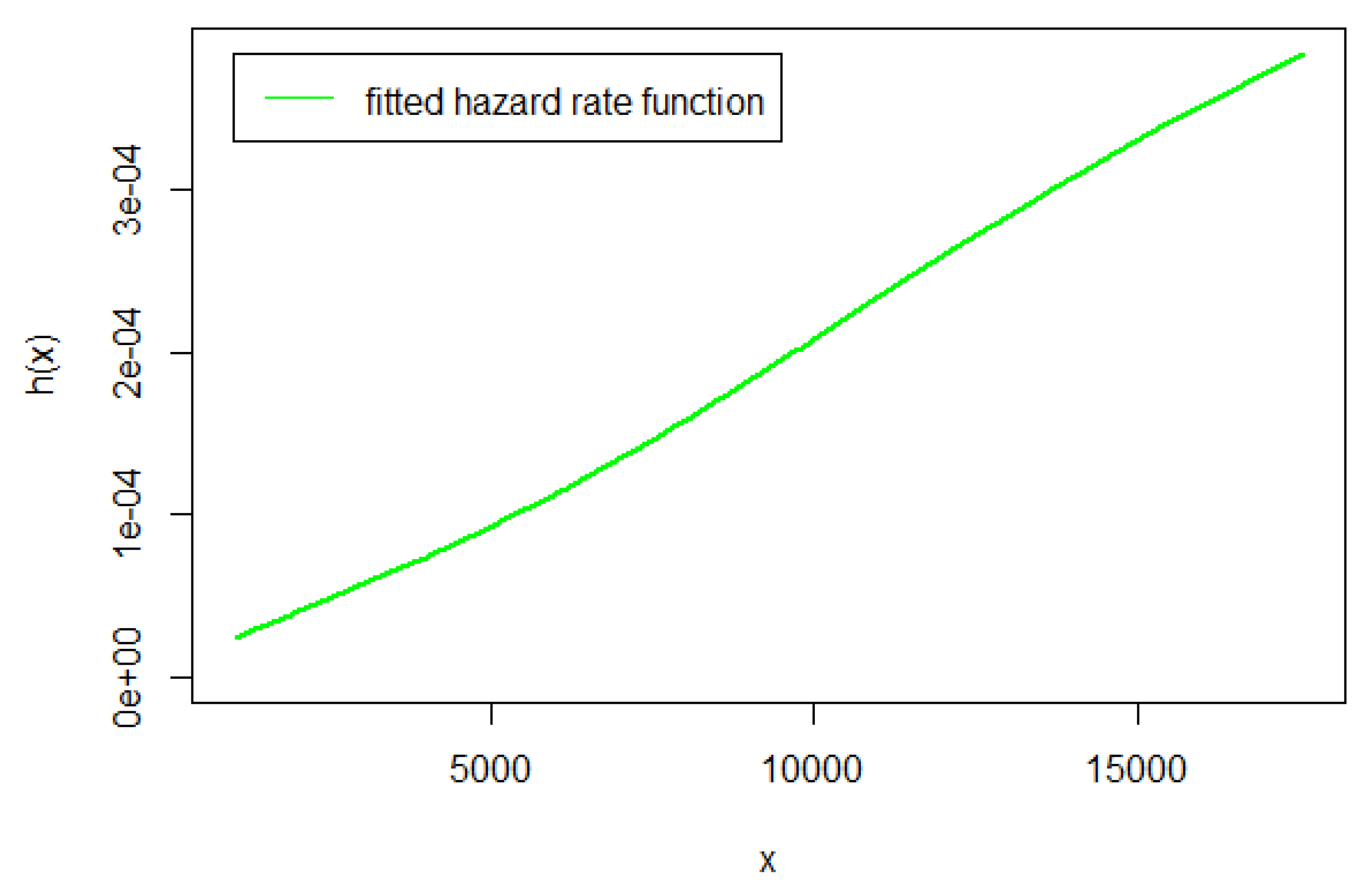

Table 1.
Quantiles of the HLNWP Distribution for Some Selected Values of Parameters , and
| () | () | () | () | () | |
| p-quantile | (0.2,1.5,0.5) | (2.6,0.6,1.1) | (1,1.1,1.2) | (1.5,0.4,2.1) | (0.5,0.9,1) |
| 0.1 | 0.5011 | 0.0154 | 0.2787 | 0.0137 | 0.3626 |
| 0.2 | 0.8009 | 0.0497 | 0.5282 | 0.0798 | 0.7923 |
| 0.3 | 1.0619 | 0.1006 | 0.7760 | 0.2298 | 1.2678 |
| 0.4 | 1.3091 | 0.1698 | 1.0322 | 0.5036 | 1.7969 |
| 0.5 | 1.5566 | 0.2617 | 1.3071 | 0.9641 | 2.3981 |
| 0.6 | 1.8177 | 0.3857 | 1.6149 | 1.7244 | 3.1052 |
| 0.7 | 2.1107 | 0.5603 | 1.9799 | 3.0199 | 3.9834 |
| 0.8 | 2.4710 | 0.8309 | 2.4546 | 5.4535 | 5.1801 |
| 0.9 | 3.0035 | 1.3534 | 3.2029 | 11.3370 | 7.1712 |
Table 2.
Moments of the HLNWP Distribution for Some Selected Values of Parameters , and .
| () | () | () | () | () | |
| (0.2,1.5,0.5) | (2.6,0.6,1.1) | (1,1.1,1.2) | (1.5,0.4,2.1) | (0.5,0.9,1) | |
| 0.1637 | 0.2312 | 0.1980 | 0.1320 | 0.1147 | |
| 0.1162 | 0.1220 | 0.1320 | 0.0744 | 0.0747 | |
| 0.0899 | 0.0806 | 0.0987 | 0.0516 | 0.0553 | |
| 0.0733 | 0.0596 | 0.0787 | 0.0394 | 0.0439 | |
| 0.0618 | 0.0471 | 0.0654 | 0.0319 | 0.0364 | |
| SD | 0.2989 | 0.2618 | 0.3046 | 0.2387 | 0.2480 |
| CV | 1.8257 | 1.1323 | 1.5386 | 1.8085 | 2.1620 |
| CS | 1.5582 | 1.1547 | 1.2678 | 1.9656 | 2.1376 |
| CK | 3.8732 | 3.3202 | 3.1341 | 5.8733 | 6.3114 |
Table 3.
Monte Carlo Simulation Results: Average Bias, RMSE, CP and AW
| I(=2.0, =2.5) | II(=0.5, =0.5) | |||||||||
| Parameter | n | Average Bias | RMSE | CP | AW | Average Bias | RMSE | CP | AW | |
| 25 | 0.04520 | 0.44965 | 0.9000 | 1.37242 | -0.02316 | 0.16337 | 0.9000 | 0.55275 | ||
| 50 | 0.04644 | 0.27205 | 0.9300 | 0.95906 | 0.00392 | 0.10158 | 0.9300 | 0.40736 | ||
| 100 | 0.04348 | 0.19837 | 0.9600 | 0.67701 | 0.00109 | 0.08169 | 0.9100 | 0.28715 | ||
| 200 | 0.01244 | 0.11401 | 0.9800 | 0.46829 | 0.00372 | 0.05405 | 0.9400 | 0.20401 | ||
| 400 | 0.00997 | 0.09441 | 0.9200 | 0.33075 | 0.00499 | 0.03912 | 0.9400 | 0.14466 | ||
| 800 | 0.00208 | 0.05984 | 0.9500 | 0.23260 | -0.00012 | 0.02664 | 0.9200 | 0.10174 | ||
| 25 | 0.19469 | 0.55050 | 0.9200 | 1.75557 | 0.03894 | 0.11010 | 0.9200 | 0.35111 | ||
| 50 | 0.05059 | 0.30160 | 0.9700 | 1.16858 | 0.01012 | 0.06032 | 0.9700 | 0.23372 | ||
| 100 | 0.05991 | 0.23210 | 0.9400 | 0.82731 | 0.01198 | 0.04642 | 0.9400 | 0.16546 | ||
| 200 | 0.00522 | 0.14750 | 0.9400 | 0.57269 | 0.00104 | 0.02950 | 0.9400 | 0.11454 | ||
| 400 | -0.00561 | 0.10749 | 0.9700 | 0.40284 | -0.00112 | 0.02150 | 0.9700 | 0.08057 | ||
| 800 | -0.00015 | 0.07587 | 0.9200 | 0.28574 | 0.00042 | 0.01517 | 0.9200 | 0.05715 | ||
Table 4.
Monte Carlo Simulation Results: Average Bias, RMSE, CP and AW
| III(=1.5,=0.5) | IV(=0.5,=1.5) | |||||||||
| Parameter | n | Average Bias | RMSE | CP | AW | Average Bias | RMSE | CP | AW | |
| 25 | 0.05737 | 0.32195 | 0.9000 | 1.08578 | -0.02315 | 0.16336 | 0.9000 | 0.55275 | ||
| 50 | 0.03005 | 0.19909 | 0.9400 | 0.75401 | 0.00391 | 0.10157 | 0.9300 | 0.40736 | ||
| 100 | 0.00353 | 0.15119 | 0.9100 | 0.52561 | 0.00109 | 0.08168 | 0.9100 | 0.28714 | ||
| 200 | -0.00749 | 0.10306 | 0.9400 | 0.36909 | 0.00372 | 0.05404 | 0.9400 | 0.20401 | ||
| 400 | 0.00003 | 0.06515 | 0.9600 | 0.26159 | 0.00499 | 0.03911 | 0.9400 | 0.14466 | ||
| 800 | 0.00003 | 0.04562 | 0.9600 | 0.18544 | -0.00012 | 0.02664 | 0.9200 | 0.10174 | ||
| 25 | 0.02705 | 0.08536 | 0.9800 | 0.34295 | 0.11681 | 0.33029 | 0.9200 | 1.05334 | ||
| 50 | 0.01475 | 0.07108 | 0.9300 | 0.23578 | 0.03035 | 0.18096 | 0.9700 | 0.70115 | ||
| 100 | 0.00859 | 0.04892 | 0.9500 | 0.16482 | 0.03594 | 0.13926 | 0.9400 | 0.49638 | ||
| 200 | 0.00201 | 0.02800 | 0.9500 | 0.11461 | 0.00313 | 0.08849 | 0.9400 | 0.34361 | ||
| 400 | 0.00428 | 0.01892 | 0.9800 | 0.08156 | -0.00336 | 0.06449 | 0.9700 | 0.24171 | ||
| 800 | 0.00046 | 0.01302 | 0.9600 | 0.05714 | 0.00125 | 0.04552 | 0.9200 | 0.17144 | ||
Table 5.
Covid-19 New Jersey Data
| 1 | 1 | 1 | 5 | 4 | 3 | 4 | 1 | 10 | 6 | 11 | 14 | 17 | 12 | 25 | 12 | 14 | 35 |
| 41 | 44 | 30 | 24 | 28 | 33 | 54 | 64 | 61 | 25 | 46 | 44 | 53 | 55 | 80 | 86 | 89 | 105 |
| 28 | 48 | 73 | 120 | 103 | 71 | 91 | 32 | 58 | 85 | 75 | 89 | 80 | 75 | 24 | 71 | 92 | 74 |
| 81 | 91 | 64 | 26 | 61 | 97 | 104 | 55 | 79 | 32 | 103 | 86 | 106 | 69 | 71 | 31 | 19 | 43 |
| 102 | 89 | 80 | 82 | 97 | 74 | 27 | 47 | 72 | 61 | 63 | 72 | 66 | 29 | 23 | 95 | 97 | 71 |
| 47 | 72 | 27 | 30 | 85 | 79 | 74 | 65 | 67 | 24 | 48 | 69 | 96 | 79 | 64 | 33 | 32 | 42 |
| 104 | 82 | 98 | 63 | 29 | 19 | 75 | 118 | 150 | 137 | 102 | 73 | 26 | 46 | 138 | 125 | 127 | 121 |
| 91 | 12 | 57 | 119 | 155 | 156 | 134 | 90 | 27 | 92 | 169 | 175 | 113 | 191 | 136 | 38 | 108 | 196 |
| 169 | 148 | 188 | 103 | 67 | 87 | 182 | 160 | 186 | 151 | 75 | 19 | 98 | 179 | 164 | 134 | 166 | 146 |
| 18 | 104 | 149 | 142 | 140 | 144 | 67 | 35 | 80 | 144 | 157 | 167 | 152 | 65 | 22 | 33 | 72 | 154 |
| 99 | 172 | 71 | 52 | 75 | 152 | 105 | 90 | 99 | 73 | 31 | 53 | 123 | 117 | 88 | 132 | 51 | 21 |
| 34 | 150 | 107 |
Table 6.
Estimates of Models for Covid-19 New Jersey Data
| Estimates | |||
| Distribution | |||
| HLNWP | 2.8384 | 0.0142 | 1.3532 |
| () | () | () | |
| HLW | 1 | 0.0035 | 1.3532 |
| (-) | (0.0013) | (0.0813) | |
| HLE | 1 | 0.0182 | 1 |
| (-) | (0.0010) | (-) | |
| HLR | 1 | 2 | |
| (-) | () | (-) | |
| HLP | 54.9957 | 1 | 1 |
| (3.1493) | (-) | (-) | |
| NWP | 5.8136 | 0.0147 | 1.5620 |
| () | () | () | |
| MOLL | 21.8981 | 2.0480 | 9.6746 |
| (0.9138) | (0.1227) | (1.0099) | |
| MOEIW | 2.0477 | ||
| () | () | (1.4130) | |
Table 7.
Goodness-of-fit Statistics of Models for Covid-19 New Jersey Data
| Statistics | ||||||||
| Distribution | AIC | CAIC | BIC | W* | A* | SS | KS-Pvalue | |
| HLNWP | 2101.3750 | 2107.3750 | 2107.4970 | 2117.2850 | 0.1414 | 0.9068 | 0.1270 | 0.3534 |
| HLW | 2101.3750 | 2105.3750 | 2105.4350 | 2111.9810 | 0.1415 | 0.9069 | 0.1269 | 0.3529 |
| HLE | 2123.7920 | 2125.7920 | 2125.8120 | 2129.0960 | 0.2442 | 1.5016 | 1.0221 | |
| HLR | 2151.4250 | 2153.4250 | 2153.4450 | 2156.7280 | 0.0873 | 0.5916 | 1.4159 | |
| HLP | 2123.7920 | 2125.7920 | 2125.8120 | 2129.0960 | 0.2442 | 1.5016 | 1.0222 | |
| NWP | 2107.1740 | 2113.1750 | 2113.2960 | 2123.0840 | 0.2186 | 1.3386 | 0.2062 | 0.1308 |
| MOLL | 2159.5680 | 2165.5680 | 2165.6900 | 2175.4780 | 0.8486 | 4.9632 | 0.4778 | 0.0343 |
| MOEIW | 2159.5690 | 2165.5690 | 2165.6910 | 2175.4790 | 0.8508 | 4.9762 | 0.4817 | 0.0318 |
Table 8.
Kevlar70 Data
| 1051 | 1337 | 1389 | 1921 | 1942 | 2322 | 3629 | 4006 | 4012 | 4063 | 4921 | 5445 | 5620 | 5817 |
| 5905 | 5956 | 6068 | 6121 | 6473 | 7501 | 7886 | 8108 | 8546 | 8666 | 8831 | 9106 | 9711 | 9806 |
| 10205 | 10396 | 10861 | 11026 | 11214 | 11362 | 11604 | 11608 | 11745 | 11762 | 11895 | 12044 | 13520 | 13670 |
| 14110 | 14496 | 15395 | 16179 | 17092 | 17568 | 17568 |
Table 9.
Estimates of Models for Kevlar70 Data
| Estimates | |||
| Distribution | |||
| HLNWP | 22.8770 | 1.7523 | |
| () | () | () | |
| HLW | 1 | 1.7523 | |
| (-) | () | () | |
| HLE | 1 | 1 | |
| (-) | () | (-) | |
| HLR | 1 | 2 | |
| (-) | () | (-) | |
| HLP | 6059.5500 | 1 | 1 |
| (693.0200) | (-) | (-) | |
| NWP | 0.5284 | 0.0052 | 0.5459 |
| (2.0061) | (0.0135) | (0.0912) | |
| MOLL | 631.4893 | 2.6196 | 770.5876 |
| (189.9811) | (0.3166) | (59.4308) | |
| MOEIW | 438.5400 | 2.6086 | 0.0013 |
| () | () | () | |
Table 10.
Goodness-of-fit statistics of Models for Kevlar70 Data
| Statistics | ||||||||
| Distribution | AIC | CAIC | BIC | W* | A* | SS | KS-Pvalue | |
| HLNWP | 960.6601 | 966.6601 | 967.1934 | 972.3356 | 0.0564 | 0.3719 | 0.0569 | 0.9371 |
| HLW | 960.6601 | 964.6996 | 964.9605 | 968.4833 | 0.0562 | 0.3706 | 0.0695 | 0.8539 |
| HLE | 977.4480 | 979.4480 | 979.5331 | 981.3398 | 0.1062 | 0.6906 | 0.5654 | 0.0449 |
| HLR | 979.2739 | 981.2730 | 981.3581 | 983.1648 | 0.0477 | 0.3148 | 0.9104 | 0.0049 |
| HLP | 977.4480 | 979.4480 | 979.5331 | 981.3398 | 0.1062 | 0.6906 | 0.5654 | 0.0449 |
| NWP | 1035.0300 | 1041.0300 | 1041.5630 | 1046.7050 | 0.1917 | 1.2372 | 2.0615 | |
| MOLL | 974.0705 | 980.0705 | 980.6038 | 985.7459 | 0.2216 | 1.4137 | 0.1353 | 0.5642 |
| MOEIW | 974.0160 | 980.0160 | 980.5493 | 985.6914 | 0.2267 | 1.4430 | 0.1366 | 0.5573 |
Disclaimer/Publisher’s Note: The statements, opinions and data contained in all publications are solely those of the individual author(s) and contributor(s) and not of MDPI and/or the editor(s). MDPI and/or the editor(s) disclaim responsibility for any injury to people or property resulting from any ideas, methods, instructions or products referred to in the content. |
© 2025 by the authors. Licensee MDPI, Basel, Switzerland. This article is an open access article distributed under the terms and conditions of the Creative Commons Attribution (CC BY) license (http://creativecommons.org/licenses/by/4.0/).
Copyright: This open access article is published under a Creative Commons CC BY 4.0 license, which permit the free download, distribution, and reuse, provided that the author and preprint are cited in any reuse.


