
Submitted:
07 August 2025
Posted:
08 August 2025
You are already at the latest version
Abstract
The main goal of the paper is to present a new, two-version flexible distribution that is a modification of the Weibull lifetime model. An innovative idea is to replace the Weibull shape parameter with a shape function. An additional goal is to propose an estimation method that measures the absolute values of the differences between the empirical and theoretical reliability functions. An extensive literature review is performed on 165 generalizations of the Weibull distribution, considering modalities and shapes of the hazard rate function (HRF). Properties of the proposed distribution and real data examples of the application of our proposal are presented. Cumulative failure functions of the bimodal models with a bathtub HRF are given.
Keywords:
lifetime models
; Weibull distribution
; bimodal distribution
; bathtub hazard rate function
1. Introduction
Without any particular exaggeration, one may say that nearly everything in a lifetime data analysis revolves around the hazard rate function (HRF). Lifetime models (LTMs) are categorized according to the shapes of their HRFs. Special attention is paid to LTMs of “flat-bottomed” HRFs that are commonly named bathtub HRFs. Unfortunately, over time, this name has been used to describe any HRF having a minimum but evidently not being flat-bottomed. The true, i.e. flat-bottomed bathtub hazard rate, is specific to a non-homogeneous population. This population consists of subpopulations of “weak” and “strong” items.
Categorized roughly, LTMs may fall into monolithic or hybrid categories. The most representative monolithic LTMs to be recalled here seem to be the Weibull (W), Gamma (G) and Gamma Weibull (GW). Their failure density functions (FDFs) are
where is the scale parameter, are the shape parameters, is the failure free time parameter and is the step function defined as
Please note that (3) LTM came into being by embedding (1) into (2). It makes (3) more flexible than both (1) and (2) owing to the second shape parameter, namely. However, none of LTMs in question is sufficiently flexible to be applicable to non-homogeneous populations. It is because they cannot be bimodal. The reader may check it on their own.
The prime example of hybrid LTM is the compound Weibull (CW) proposed by [48]. Its FDF is given by
where .
As mentioned above, monolithic LTMs are unimodal. In contrast, hybrid LTMs may be bimodal. Of course, they can also be unimodal when (1) or (2), to the great surprise of the analyst, turns out to be inapplicable to a homogeneous population. Struck by the superiority of (5) over (1), (2), (3) one must not overlook the fact that (5) has twice as many parameters than (3). Therefore, employing (5) one should have at its disposal much more input data than employing (3). It is essential to guarantee that (5) and (3) sets of estimates are at the same level of accuracy. We face the problem of equilibrating flexibility and data consumption.
To familiarize ourselves with the problem, let us consider the results of the following simple, but very instructive, Monte Carlo experiment. A set of input data that comprises one hundred samples each of 30 items were drawn from the exponential population. The population scale parameter was set equal to one. Then (1), (2), (3) LTMs were sequentially fitted to the data set. Parameters were estimated with the Maximum Likelihood (ML) Method. Table 1 shows standard deviations of scale parameter estimates.
The (3) LTM produced scale parameter estimates of standard deviation more than five times greater than the (1) LTM did. The explanation is simple. Saying freely, “underfeeding” of the scale parameter took place because the shape parameters have “eaten” most of the input data for their estimation purposes.
In general, no one disputes the need for LTM to be flexible. On the other hand, does LTM need to have as many as 8 parameters? The LTM below, called Kumaraswamy transmuted exponentiated additive Weibull (KTEAW) [66], satisfies the mentioned criterion. Cumulative failure function (CFF) of the KTEAW is defined as
where
In general, there are currently two techniques to increase flexibility of LTM: In the formula of the failure density function there are embed more parameters or the same parameter are embedded in more than one place. The reader is prompted to compare (1) with (2). The Weibull distribution turned out to be a little more flexible than the Gamma distribution in Monte Carlo experiments.
The shape parameter can be called static in a sense that it shapes the LTM identically at each time point. In this paper, we will be able to shape LTM dynamically owing to the following modification: we replace the shape parameter with the shape function. This is an innovative idea. The subject of modification, of course, will be the Weibull LTM further named the Weibull distribution with shape function (WDSF). The CFF and FDF take forms:
The above FDF is a sum of two components. This is a unique property of the LTM in question. Although born as a monolithic LTM the WDSF turns out to be hybrid-like LTM. Please note that WDSF is free of the fraction parameter , which is a data guzzler in (5). As it is easy to guess, we, further in this paper, consider the simplest version of WDSF that involves a linear shape function.
By the end of this section, let us return to the very origins of the reliability domain. Let us recall two books published by reliability pathfinders of that time. These are [39] and [46]. A device stops working properly, not because the Finger of Fate points it out and says “fail”. It does it because physical failure process reached its critical level. In mentioned books, commonly used LTM have assigned a particular mathematical failure mechanism or process.
For instance, both books assign the Weibull LTM to the model of weakest link of the chain of elements forming a very long series reliability structure. This point of view appears to be timeless. Therefore, in this paper we have the courage to extend the Weibull LTM assigning the following failure process: As time flows and wear-out process advances, series reliability structure steadily elongates causing device reliability to decrease. Referential mathematical consideration will be presented in Section Properties of Weibull distribution with shape function.
The main goal of our work is to complement the literature on the theory of reliability models by introducing a new distribution with a linear shape function, which is a modification of the Weibull LTM. The additional goal of our paper is to define an estimation method that measures the absolute values of the differences between the empirical and theoretical reliability functions (RF) (see Section Estimation methods).
The rest of the paper is organized as follows. Section A review of modified Weibull distributions is devoted to the review of modified Weibull distributions. The properties of the two-version WDSF such as the CFF, RF, FDF, HRF, hazard rate average function (HRAF), quantile (Q) and pseudo-random number generator (PRNG) are described in Section Properties of Weibull distribution with shape function. Used estimation methods are described in Section Estimation methods. Illustrative examples of applicability and flexibility of the WDSF are presented in Section Applications. Concluding remarks are provided in Conclusions. CFF formulas of bimodal LTMs defined with 5–8 parameters and having a bathtub HRF are provided in Appendix A. As the popularity of the R environment has increased significantly recently, main properties of the new distribution have been implemented in R software [75]. Their full codes are in Appendix B.
2. A Review of Modified Weibull Distributions
Generalized Weibull distributions can be constructed in many ways. The first, and in our opinion, the most important way is to define distributions with the Weibull distribution as their special case (including a mixture of two or more Weibull variables). Other ways are i.e.: adding a constant to the hazard rate of the Weibull model; transformations (linear, inverse or log) of the Weibull random variable; transformations of the CFF or survival function of the Weibull models in such a way that the new models remains a CFF or survival function. More details can be found in [54].
By reviewing the statistical literature, we found 165 generalized Weibull distributions with 2 – 8 parameters. Among them, four distributions have a domain different from . There are: reflected Weibull distribution [26] defined for as well as the Log-Weibull [41]; [11], modified odd Weibull Normal [25] and extended odd Weibull normal [7] distributions defined for .
In the rest of the Section, we will focus on such generalized Weibull distributions, for which the Swedish research’s distribution is their special case. In this case, the large family of generalized Weibull distributions reduces to 71 distributions with 3–8 parameters, named by the authors as modified Weibull distributions.
Modified Weibull distributions are divided into six groups, according to the number of their parameters. The list of these models is presented below. Information on hazard rate function shapes is provided in the superscript (1unimodal, 2increasing, 3decreasing, 4bathub). Pseudo-bimodal lifetime models with bathtub hazard rate function are in underline (22 models). Bimodal lifetime models with bathtub hazard rate function are in bold (7 models) and their CFFs are presented in Appendix A.
The group I includes 19 models with three parameters. There are: generalized gamma or gamma Weibull1−4 [87], generalization of gamma Weibull1−4 [88], exponentiated Weibull1−4 [60], Generalized Weibull1−4 [61], exponentiated Weibull1−4 [62], power generalized Weibull1−4 [20], modified Weibull extension2−4 [95], modified Weibull2−4 [52], Marshall-Olkin Extended Weibull1−4 [40], extended Weibull type1,4 [15], generalized power Weibull2−4 [65], Extended Weibull1−4 [96], Sarhan and Zaindin’s Modified Weibull2,3 [78], Weibull Geometric1−4 [23], transmuted Weibull1−4 [16], complementary Weibull geometric1−4 [91], Alpha power Weibull1−4 [63], MIT Weibull1−4 [55] and Semi Modified Alpha Power Weibull Distribution [18].
The group II includes 18 models with four parameters. There are: four-parameter generalized gamma1−4 [42], additive Weibull2−4 [93], Generalized Modified Weibull1,2,4 [24], Kumaraswamy Weibull1−4 [27], Exponentiated Generalized Gamma1,4 [28], exponentiated modified Weibull1−4 [36], Transmuted modified Weibull2 [50], Exponentiated transmuted Weibull2−4 [34], Generalized Weibull- Exponential [77]1−3, Weibull Lomax2,3 [89], generalized power generalized Weibull1−4 [80], Generalization of Generalized Gamma1−4 [84], Weibull Lomax2−4 [69], additive Chen-Weibull2,4 [90], Poisson modified Weibull1−4 [2], modified power generalized Weibull1−4 [83], Generalized New Extended Weibull [13] and new modified exponentiated Weibull (NMEW) [74]2,4.
The group III includes 27 models with five parameters. There are: Beta modified Weibull1−4 [86], Kumaraswamy generalized gamma1−4 [73], beta generalized Weibull1−4 [85], Transmuted Exponentiated Modified Weibull2,3 [38], Beta Generalized Gamma1−4 [29], transmuted additive Weibull2,4 [37], Exponentiated Kumaraswamy Weibull1−4 [35], new modified Weibull2−4 [10], Kumaraswamy modified Weibull1−4 [31], beta transmuted Weibull1−3 [70], McDonald Weibull1−4 (McW)[30], Exponentiated Transmuted Modified Weibull1,2.4 [71], exponentiated generalized modified Weibull2,4 [17], gamma generalized modified Weibull[67], generalized modified Weibull geometric4 [21], additive modified Weibull2−4 [44], transmuted exponentiated Weibull geometric1−4 [76], transmuted new generalized Weibull2−3 [51], Burr XII modified Weibull1−4 [56], log-logistic modified Weibull1,2,4 [68], Kumaraswamy alpha power Weibull1−4 [57], exponentiated additive Weibull1−4 (EAW) [9]; [4], generalized extended exponential Weibull1−4 [82], generalized Weibull generalized exponential [19]1−2, new generalized modified Weibull1−4 [8] and improved modified Weibull3,4 [47].
The group IV includes 7 models with six parameters. There are: the mixture of two Weibull4 [48], McDonald modified Weibull1−4 (McMW) [58], McDonald extended Weibull1−4 (McEW) [43], Additive Weibull log logistic1−4 [45], underbarBeta exponentiated modified Weibull1−4 [81], exponentiated power generalized Weibull binomial1−4 [6], and McDonald Generalized Power Weibull1−4 (McGPW) [79].
Concluding the review of modified Weibull distributions, we would like to mention two distributions with seven and eight parameters, respectively. Kumaraswamy transmuted exponentiated modified Weibull1−4 (KTEMW) with 54 special cases forms group V [5]. Kumaraswamy transmuted exponentiated additive Weibull1−4 (KTEAW) [66] with 79 special cases (including KTEMW) forms group VI.
3. Properties of Weibull Distribution with Shape Function
The main goal of the paper is to present the two-version Weibull distribution with the shape function previously denoted as WDSF. This section describes its properties such as CFF, RF, FDF, HRF, hazard rate average function (HRAF), quantile (Q), and pseudorandom number generator (PRNG). Both versions of our model will be used in Section Applications.
We assume that the device of our interest has a long series reliability structure. It makes the real lifetime distribution close to the Weibull distribution. The formula below is the Weibull LTM with the elongation coefficient of the device’s reliability structure.
We impose two weak conditions on with and . Owing to such weak conditions, a wide scope open itself for defining functions not only of reasonable forms but also of monstrous ones. One reasonable form is because it introduces only one parameter into the Weibull LTM and therefore equilibrates flexibility and data consumption. Thus, we get:
Definition 1.
Let from (7) or (8) be a linear shape function with two parameters given by then the CFF of the Weibull distribution with linear shape function in the first version (WDSFI) is defined as
where , is the scale parameter, are the shape parameters and (see the proof of Theorem 2). If then we get the Weibull distribution.
Definition 2.
Let from (7) or (8) be a linear shape function with three parameters given by then the CFF of the Weibull distribution with linear shape function in the second version (WDSFII) has the form
where , is the failure free time parameter, is the step function (4) and (see the proof of Theorem 2). If then we get the first vesion of our proposal.
Theorem 1.
The RFs of the WDSFI and WDSFII are defined, respectively, as
Proof of Theorem 1.
The proof based on the RF definition is trivial. □
Theorem 2.
The FDFs of the WDSFI and WDSFII are respectively given by
where .
Proof of Theorem 2.
By computing the derivatives based on (9) and (10) with respect to the lifetime t, we easily obtain formulas (13) and (14). Recall that and the formulas (13)-(14) are non-negative.
Let , then we have from (13)
Let , then we have from (14)
□
Figure 1 shows the RF of the WDSFI and WDSFII. Pseudo-bimodality or bimodality is visible here. The R codes (R Core Team 2021) for calculating the RF values of the WDSFII are provided in Appendix B.
Figure 2 shows the FDF of the WDSFI and WDSFII. We see the pseudo-bimodality (on the left) and bimodality (on the right). The R codes for calculating the FDF values of WDSFII are provided in Appendix B.
Theorem 3.
The HRFs of the WDSFI and WDSFII have respectively form
Proof of Theorem 3.
The proof based on the HRF defintion is trivial. □
Figure 3 shows the bathtub HRF of the WDSFI and WDSFII. The curves flatten as c decreases. The R codes for calculating the HRF values of WDSFII are provided in Appendix B.
Theorem 4.
The HRAFs of the WDSFI and WDSFII are respectively defined as (Barlow and Proschan 1996)
Proof of Theorem 4.
The proof based on the formula is trivial. □
Figure 4 shows the bathtub HRAF of the WDSFI and WDSFII. HRAF curves are flatter than HRF curves. The R codes for calculating the HARF values of WDSFII are provided in Appendix B.
Theorem 5.
Let . The Qs and of the WDSFI and WDSFII are respectively solutions of the equations
The R codes for calculating the values of WDSFII are provided in Appendix B.
Theorem 6.
Let , and follow the WDSFI and WDSFII, respectively. We can obtain the and in two ways.
The first way. The and are respectively solutions of the equations
The second way. The algorithm for obtaining the and is as follows:
- 1.
- Let , , .
- 2.
- Let
- 3.
- , .
- 4.
- If , then go to step 2.
- 5.
- Return , .
Proof of Theorem 6.
The R codes for the PRNG of the WDSFII are provided in Appendix B.
4. Estimation Methods
Additional goal for this article is outlined in this Section.
Looking through the literature in search of distributions that are modifications of the Weibull distribution, we find that the most dominant method of parameter estimation is the maximum likelihood (ML) method. However, the question remains whether this choice is right. The younger the paper, the more often the parameters are estimated using other methods, e.g. the ordinary least-squares (LS) and weighted least-squares (WLS) ones, see e.g. [3]; [64]; [14]; [12]; [83].
Let be parameter vectors and be a random sample of size n from the WDSFI and WDSFII. To estimate unknown values of parameters, we use estimation methods such as the ML, LS, WLS and least absolute values (LAW). The LAW, which is the first additional goal of the work, measures the absolute values of the differences between the empirical and theoretical RFs.
The likelihood functions (LFs) of the WDSFI and WDSFII, based on (13-14), are given by, respectively
where .
The log-likelihood functions (LLFs) of the WDSFI and WDSFII, based on ((25)-(26)), are defined as, respectively
Formulas have complex forms, so in practice we maximize the LF (27-28) or the LLFs (29-30) to obtain the ML estimates.
To obtain the OLS estimates of the WDSFI and WDSFII parameters, we minimize the following objective functions, respectively
To obtain the WLS estimates of the WDSFI and WDSFII parameters, we minimize the following objective functions, respectively
Let is the empirical RF. To obtain the LAW estimates of the WDSFI and WDSFII parameters, we minimize the following objective functions, respectively
Simulation study was performed with samples with a size of . The samples were drawn from the WDSFII with , where . To obtain highly accurate parameter estimates, the optimization procedure was run times with random initial values of for and for . Our estimates for a given sample are the values that minimize (29), (31), (33) and maximize (27).
The biases and the root mean squared errors (RMSEs) of the WDSFII estimates are shown in Table 2. We observe that as the sample size increases, the estimates approach the true values, which means that the estimates are consistent. Biases and RMSE values are the lowest for . The biases are the largest for ( and (. The RMSEs are the highest for . The biases increase with the value of c for . The RMSEs increase with the value of c for and decrease for . The biases are the lowest for the ML method associated with . The biases are lowest for the ML method associated with . The ML method is not suitable for estimating scale parameters.
5. Applications
In this section, we illustrate the importance of the WDSFI and WDSFII distributions using three real life data sets. The new models are compared with bimodal LTMs, characterized by unimodal, increasing, decreasing and bathub HRF, such as: exponentiated additive Weibull, McDonald Weibull, McDonald modified Weibull, McDonald extended Weibull, McDonald generalized Power Weibull, Compound Weibull, Kumaraswamy transmuted exponentiated modified Weibull, Kumaraswamy transmuted exponentiated additive Weibull. CFFs of mentioned models are presented in Appendix.
All calculations for comparison were performed in R software. To avoid local maxima, the optimization procedure was run times with random starting model parameter values that are widely scattered in the parameter space. The final parameter estimates are those parameter values that best maximize the log-likelihood function. AIC, BIC, HQIC criteria and the Kolmogorov-Smirnov (KS) statistic are calculated.
5.1. Failure times of devices
As the first real dataset, 50 failure times of devices ([1]; [53]) presented in Appendix C, is used. ML estimates (MLEs), AIC, BIC, HQIC and KS values are given in Table 3. Better values are marked in bold. Figure 5 shows the estimated FDFs for compared models. The WDSFII model is more appropriate based on information criteria and KS values. The adaptability of the WDSFII model can also be observed in Figure 5.
5.2. 500 MW generators
As the second real dataset, 36 times to the first failure of 500 MW generators collected over a 6-year period ([33]; [53]) presented in Appendix C, is used. ML estimates (MLE), AIC, BIC, HQIC and KS values are given in Table 4. The WDSFI model is more appropriate based on information criteria. The adaptability of the WDSFI model can also be observed in Figure 6.
6. Discussion
The results obtained in this study demonstrate that the proposed WDSFI and WDSFII models provide a flexible and accurate framework for modeling full-life-cycle data with a wide range of hazard ratio shapes, including monotonic, bathtub, and pseudobimodal patterns. Parameter estimation using OLS, WLS, and LAW methods yielded consistent results, with the LAW approach often demonstrating improved robustness in the presence of irregularities in the empirical reliability function.
From the perspective of previous research, our findings are consistent with, and even extend, previous work on generalizations of the Weibull distribution and its modified forms. Similar to these studies, we observed that introducing additional parameters can significantly improve model fit, allowing for more complex hazard ratio shapes. However, the WDSFI and WDSFII models differ in structure, offering better adaptation to datasets where existing models still exhibit systematic biases.
Regarding our working hypotheses, empirical analyses support the assumption that additional flexibility in scale structure and distribution shape leads to better data representation without sacrificing interpretability. The models’ performance on real-world datasets suggests they may be particularly well-suited for applications in engineering reliability, biomedical survival analysis, and materials degradation studies, where multi-phase failure mechanisms are present.
In a broader context, these findings contribute to the growing literature on extended-life models and highlight the continuing need for statistical tools capable of capturing a variety of hazardous behaviors. Such tools are crucial for risk assessment, preventive maintenance planning, and decision-making in safety-critical systems.
Future research directions include:
- Extending the proposed models to more precisely process censored, truncated, and interval data.
- Investigation of Bayesian inference methods to incorporate a priori information and quantify uncertainty.
- Development of multivariate or concatenated life-cycle models to capture inter-component dependencies.
- Incorporation of models into regression frameworks, such as proportional hazards or accelerated failure time models, to assess the impact of interdependent variables.
Overall, this study confirms the practical value of the WDSFI and WDSFII models and opens promising avenues for both theoretical development and applied research in reliability and survival analysis.
7. Conclusions
This article presents a three- and four-parameter flexible modified Weibull LTM called the Weibull distribution with a linear shape function. An innovative idea is to replace the Weibull shape parameter with a shape function. An estimation method based on theoretical and empirical reliability functions is proposed. An extensive literature review was performed, taking into account the modalities and shapes of the risk rate function. The simulation study is carried out using ML, LS, WLS and LAW methods. Furthermore, to check the suitability and flexibility, the new LTMs are validated with two real datasets and compared with other bimodal LTMs with a bathtub HRF.
The paper shows that even a three-parameter distribution can compete in data modeling with LTM distributions that have two or even almost three times more parameters.
Author Contributions
Conceptualization, P.S. and A.D.; methodology, P.S. and A.D.; software, P.S.; validation, P.S.; formal analysis, P.S and A.D.; investigation, P.S.; resources, P.S and A.D.; data curation, P.S.; writing—original draft preparation, P.S.; writing—review and editing, P.S. and A.D; visualization, P.S.; supervision, A.D.; project administration, P.S and A.D. All authors have read and agreed to the published version of the manuscript.
Institutional Review Board Statement
The study was conducted in accordance with the Declaration of Helsinki, and did not involve humans or animals.
Data Availability Statement
R codes for the RF, CFF, FDF, HRF, HRAF, quantile and pseudo-random number generator are available at github.com/PiotrSule/WDSF.
Conflicts of Interest
The authors declare no conflicts of interest. There were no funders.
Abbreviations
The following abbreviations are used in this manuscript:
| CFF | Cumulative failure function |
| CW | Compound Weibull |
| EAW | Exponentiated additive Weibull |
| FDF | Failure density function |
| G | Gamma |
| GW | Gamma Weibull |
| HRAF | Hazard rate average function |
| HRF | Hazard rate function |
| KTEAW | Kumaraswamy transmuted exponentiated additive Weibull |
| KTEAW | Kumaraswamy transmuted exponentiated additive Weibull |
| KTEMW | Kumaraswamy transmuted exponentiated modified Weibull |
| LAW | Least Absolute Weighted |
| LLF | Log-likelihood function |
| LTM | Lifetime model |
| McGPW | McDonald Generalized Power Weibull |
| McMW | McDonald modified Weibull |
| McW | McDonald Weibull |
| ML | Maximum Likelihood |
| NMEW | New modified exponentiated Weibull |
| OLS | Ordinary least squares |
| PRNG | Pseudo-random number generator |
| Q | Quantile |
| RF | Reliabity function |
| W | Weibull |
| WDSF | Weibull distribution with shape function |
| WLS | Weighted least squares |
Appendix A.
Let be the model parameters and
- 1.
- Beta function: ,
- 2.
- Lower incomplete beta function: ,
- 3.
- Regularized incomplete beta function: .
Below are the CFFs of bimodal LTMs with unimodal, increasing, decreasing and bathub HRF. The number of model parameters is given in parentheses.
- 1.
- exponentiated additive Weibull (5)
- 2.
- McDonald Weibull (5)
- 3.
- McDonald modified Weibull (6)
- 4.
- McDonald extended Weibull (6)
- 5.
- McDonald generalized Power Weibull (6)
- 6.
- Compound Weibull (6)
- 7.
- Kumaraswamy transmuted exponentiated modified Weibull (8)
- 8.
- Kumaraswamy transmuted exponentiated additive Weibull (8)
Appendix B.
R codes for the RF, CFF, FDF, HRF, HRAF, quantile and pseudo-random number generator are available at github.com/PiotrSule/WDSF.
Appendix C.
Dataset of failure times of 50 devices:
Dataset of 36 times to the first failure of 500 MW generators collected over a 6-year period:
References
- Aarset, M.V. How to identify a bathtub hazard rate. IEEE Trans. Reliab. 1987, 36, 106–108.
- Abd El-Monsef, M.M.E.; Marei, G.A.; Kilany, N.M. Poisson modified Weibull distribution with inferences on stress-strength reliability model. Qual. Reliab. Eng. Int. 2022, 38, 2649–2669.
- Afify, A.Z.; Mohamed, O.A. A new three-parameter exponential distribution with variable shapes for the hazard rate: Estimation and applications. Mathematics 2020, 8, 135.
- Ahmad, A.A.; Ghazal, M.G.M. Exponentiated additive Weibull distribution. Reliab. Eng. Syst. Saf. 2020, 193, 106663.
- Al-Babtain, A.; Fattah, A.A.; Ahmed, A.H.N.; Merovci, F. The Kumaraswamy-transmuted exponentiated modified Weibull distribution. Commun. Stat. Simul. Comput. 2017, 46, 3812–3832.
- Aldahlan, M.A.; Jamal, F.; Chesneau, C.; Elbatal, I.; Elgarhy, M. Exponentiated power generalized Weibull power series family of distributions: Properties, estimation and applications. PLoS One 2020, 15(3).
- Alizadeh, M.; Altun, E.; Afify, A.Z.; Ozel, G. The extended odd Weibull-G family: properties and applications. Commun. Fac. Sci. Univ. Ankara Ser. A1 Math. Stat. 2018, 68(1), 161–186.
- Alizadeh, M.; Khan, M.N.; Rasekhi, M.; Hamedani, G.G. A new generalized modified Weibull distribution. Stat. Optim. Inf. Comput. 2021, 9(1), 17–34.
- Aljouiee, A.; Elbatal, I.; Al-Mofleh, H. A new five-parameter lifetime model: Theory and applications. Pak. J. Stat. Oper. Res. 2018, 14(2), 403–420.
- Almalki, S.J.; Yuan, J. A new modified Weibull distribution. Reliab. Eng. Syst. Saf. 2013, 111, 164–170.
- Almalki, S.J.; Nadarajah, S. Modifications of the Weibull distribution: A review. Reliab. Eng. Syst. Saf. 2014, 124, 32–55.
- Almetwally, E.M. The odd Weibull inverse Topp–Leone distribution with applications to COVID-19 data. Ann. Data Sci. 2022, 9(1), 121–140.
- Al-Moisheer, A.S.; Sultan, K.S.; Radwan, H.M. A novel adaptable Weibull distribution and its applications. Axioms 2025, 14(7), 490.
- Almongy, H.M.; Almetwally, E.M.; Aljohani, H.M.; Alghamdi, A.S.; Hafez, E.H. A new extended Rayleigh distribution with applications of COVID-19 data. Results Phys. 2021, 23, 104012.
- Al-Saleh, J.A.; Agarwal, S.K. Extended Weibull type distribution and finite mixture of distributions. Stat. Methodol. 2006, 3, 224–233.
- Aryal, G.; Tsokos, C.P. Transmuted Weibull distribution: A generalization of the Weibull probability distribution. Eur. J. Pure Appl. Math. 2011, 4(2), 89–102.
- Aryal, G.; Elbatal, I. On the exponentiated generalized modified Weibull distribution. Commun. Stat. Appl. Methods 2015, 22(4), 333–348.
- Azam, S.; Iqbal, M.; Zaman, Q.; Ali, M. Semi Modified Alpha Power Weibull Distribution and Its Statistical Properties. Metall. Mater. Eng. 2025, 31(2), 104–113.
- Badmus, N.I.; Olanrewaju, F. Modeling lifetime data by generalized Weibull-generalized exponential distribution. Asian J. Probab. Stat. 2020, 9(4), 65–75.
- Bagdonavicius, V.; Nikulin, M. Accelerated Life Models: Modeling and Statistical Analysis; CRC Press: Boca Raton, FL, USA, 2001.
- Bagheri, S.F.; Samani, E.B.; Ganjali, M. The generalized modified Weibull power series distribution: Theory and applications. Comput. Statist. Data Anal. 2016, 94, 136–160.
- Barlow, R.E.; Proschan, F. Mathematical Theory of Reliability; SIAM: Philadelphia, PA, USA, 1996.
- Barreto-Souza, W.; de Morais, A.L.; Cordeiro, G.M. The Weibull-geometric distribution. J. Stat. Comput. Simul. 2011, 81(5), 645–657.
- Carrasco, J.M.; Ortega, E.M.; Cordeiro, G.M. A generalized modified Weibull distribution for lifetime modeling. Comput. Statist. Data Anal. 2008, 53(2), 450–462.
- Chesneau, C.; El Achi, T. Modified odd Weibull family of distributions: Properties and applications. J. Indian Soc. Probab. Stat. 2020, 21, 259–286.
- Cohen, A.C. The reflected Weibull distribution. Technometrics 1973, 15, 867–873.
- Cordeiro, G.M.; Ortega, E.M.; Nadarajah, S. The Kumaraswamy Weibull distribution with application to failure data. J. Franklin Inst. 2010, 347(8), 1399–1429.
- Cordeiro, G.M.; Ortega, E.M.; Silva, G.O. The exponentiated generalized gamma distribution with application to lifetime data. J. Stat. Comput. Simul. 2011, 81(7), 827–842.
- Cordeiro, G.M.; Castellares, F.; Montenegro, L.C.; de Castro, M. The beta generalized gamma distribution. Statistics 2013, 47(4), 888–900.
- Cordeiro, G.M.; Hashimoto, E.M.; Ortega, E.M. The McDonald Weibull model. Statistics 2014, 48(2), 256–278.
- Cordeiro, G.M.; Ortega, E.M.; Silva, G.O. The Kumaraswamy modified Weibull distribution: theory and applications. J. Stat. Comput. Simul. 2014, 84(7), 1387–1411.
- Davis, D.J.F. An analysis of some failure data. J. Amer. Statist. Assoc. 1952, 47(258), 113–150.
- Dhillon, B.S. Life distributions. IEEE Trans. Reliab. 1981, 30(5), 457–460.
- Ebraheim, A.N.E. Exponentiated transmuted Weibull distribution: A generalization of the Weibull distribution. Int. J. Math. Comput. Sci. 2014, 8(6), 903–911.
- Eissa, F.H.; Abdulaziz, R.K. The exponentiated Kumaraswamy–Weibull distribution with application to real data. Int. J. Stat. Probab. 2017, 6(6), 167–182.
- Elbatal, I. Exponentiated Modified Weibull distribution. Econ. Qual. Control 2011, 26(2), 189–200.
- Elbatal, I.; Aryal, G. On the transmuted additive Weibull distribution. Austrian J. Stat. 2013, 42(2), 117–132.
- Eltehiwy, M.; Ashour, S. Transmuted exponentiated modified Weibull distribution. Int. J. Basic Appl. Sci. 2013, 2(3), 258–269.
- Gertsbakh, I.; Kordonskiy, K.B. Models of Failure; Springer: Berlin/Heidelberg, Germany, 2012.
- Ghitany, M.E.; Al-Hussaini, E.K.; Al-Jarallah, R.A. Marshall–Olkin extended Weibull distribution and its application to censored data. J. Appl. Stat. 2005, 32(10), 1025–1034.
- Gumbel, E.J. Statistics of Extremes; Columbia University Press: New York, NY, USA, 1958.
- Harter, H.L. Maximum-likelihood estimation of the parameters of a four-parameter generalized gamma population from complete and censored samples. Technometrics 1967, 9, 159–165.
- Hashimoto, E.M.; Ortega, E.M.; Cordeiro, G.M.; Pascoa, M.A. The McDonald extended Weibull distribution. J. Stat. Theory Pract. 2015, 9, 608–632.
- He, B.; Cui, W.; Du, X. An additive modified Weibull distribution. Reliab. Eng. Syst. Saf. 2016, 145, 28–37.
- Hemeda, S. Additive Weibull log logistic distribution: properties and application. J. Adv. Res. Appl. Math. Stat. 2018, 3(4), 8–15.
- Ireson, W.G. Reliability Handbook. Part 2. By Kao, J.H.K.; McGraw-Hill: Toronto, ON, Canada; London, UK; Sydney, Australia, 1966.
- Jiang, D.; Han, Y.; Cui, W.; Wan, F.; Yu, T.; Song, B. An improved modified Weibull distribution applied to predict the reliability evolution of an aircraft lock mechanism. Probabilist. Eng. Mech. 2023, 72, 103449.
- Kao, J.H. A graphical estimation of mixed Weibull parameters in life-testing of electron tubes. Technometrics 1959, 1(4), 389–407.
- Kenney, J.; Keeping, E. Mathematics of Statistics, Vol. 1; D. Van Nostrand Company: Princeton, NJ, USA, 1962.
- Khan, M.S.; King, R. Transmuted modified Weibull distribution: A generalization of the modified Weibull probability distribution. Eur. J. Pure Appl. Math. 2013, 6(1), 66–88.
- Khan, M.S.; King, R.; Hudson, I.L. Transmuted new generalized Weibull distribution for lifetime modeling. Commun. Stat. Appl. Methods 2016, 23(5), 363–383.
- Lai, C.D.; Xie, M.; Murthy, D.N.P. A modified Weibull distribution. IEEE Trans. Reliab. 2003, 52(1), 33–37.
- Lai, C.D.; Xie, M. Stochastic Ageing and Dependence for Reliability; Springer: Berlin/Heidelberg, Germany, 2006.
- Lai, C.D. Generalized Weibull Distributions; Springer: Berlin/Heidelberg, Germany, 2014.
- Lone, M.A.; Dar, I.H.; Jan, T.R. A new family of generalized distributions with an application to Weibull distribution. Thailand Statistician 2024, 22(1), 1–16.
- Mdlongwa, P.; Oluyede, B.; Amey, A.; Huang, S. The Burr XII modified Weibull distribution: model, properties and applications. Electron. J. Appl. Stat. Anal. 2017, 10(1), 118–145.
- Mead, M.E.; Afify, A.; Butt, N.S. The modified Kumaraswamy Weibull distribution: properties and applications in reliability and engineering sciences. Pak. J. Stat. Oper. Res. 2020, 433–446.
- Merovci, F.; Elbatal, I. The McDonald modified Weibull distribution: properties and applications. arXiv 2013, arXiv:1309.2961.
- Moors, J.J.A. A quantile alternative for kurtosis. J. R. Stat. Soc. Ser. D 1988, 37(1), 25–32.
- Mudholkar, G.S.; Srivastava, D.K. Exponentiated Weibull family for analyzing bathtub failure-rate data. IEEE Trans. Reliab. 1993, 42(2), 299–302.
- Mudholkar, G.S.; Kollia, G.D. Generalized Weibull family: a structural analysis. Commun. Stat. Theory Methods 1994, 23(4), 1149–1171.
- Mudholkar, G.S.; Srivastava, D.K.; Freimer, M. The exponentiated Weibull family: A reanalysis of the bus-motor-failure data. Technometrics 1995, 37(4), 436–445.
- Nassar, M.; Alzaatreh, A.; Mead, M.; Abo-Kasem, O. Alpha power Weibull distribution: Properties and applications. Commun. Stat. Theory Methods 2017, 46(20), 10236–10252.
- Nassar, M.; Afify, A.Z.; Shakhatreh, M.K.; Dey, S. On a new extension of Weibull distribution: Properties, estimation, and applications to one and two causes of failures. Qual. Reliab. Eng. Int. 2020, 36(6), 2019–2043.
- Nikulin, M.; Haghighi, F. A chi-squared test for the generalized power Weibull family for the head-and-neck cancer censored data. J. Math. Sci. 2006, 133(3).
- Nofal, Z.M.; Afify, A.Z.; Yousof, H.M.; Granzotto, D.C.; Louzada, F. Kumaraswamy transmuted exponentiated additive Weibull distribution. Int. J. Stat. Probab. 2016, 5(2), 78–99.
- Oluyede, B.; Huang, S.; Yang, T. A new class of generalized modified Weibull distribution with applications. Austrian J. Stat. 2015, 44(3), 45–68.
- Oluyede, B.O.; Bindele, H.F.; Makubate, B.; Huang, S. A new generalized log-logistic and modified Weibull distribution with applications. Int. J. Stat. Probab. 2018, 7(3), 72–93.
- Osagie, S.A.; Osemwenkhae, J.E. Lomax-Weibull distribution with properties and applications in lifetime analysis. Int. J. Math. Sci. Optim. Theory Appl. 2020, 2020(1), 718–732.
- Pal, M.; Tiensuwan, M. The beta transmuted Weibull distribution. Austrian J. Stat. 2014, 43(2), 133–149.
- Pal, M.; Tiensuwan, M. Exponentiated transmuted modified Weibull distribution. Eur. J. Pure Appl. Math. 2015, 8(1), 1–14.
- Pamme, H.; Kunitz, H. Detection and modelling of aging properties in lifetime data. In Adv. Reliab.; Springer: Berlin/Heidelberg, Germany, 1993; pp. 291–302.
- Pascoa, M.A.P.; Ortega, E.M.M.; Cordeiro, G.M.; Paranaíba, P.F. The Kumaraswamy-generalized gamma distribution with application in survival analysis. Stat. Methodol. 2011, 8, 411–433.
- Rangoli, A.M.; Talawar, A.S.; Agadi, R.P.; et al. New modified exponentiated Weibull distribution: A survival analysis. Cureus 2025, 17(1).
- R Core Team. R: A Language and Environment for Statistical Computing; R Foundation for Statistical Computing: Vienna, Austria, 2021. Available online: https://www.R-project.org/ (accessed on 5 August 2025).
- Saboor, A.; Elbatal, I.; Cordeiro, G.M. The transmuted exponentiated Weibull geometric distribution: Theory and applications. Hacet. J. Math. Stat. 2016, 45(3), 973–987.
- Salem, H.M.; Selim, M.A. The generalized Weibull-exponential distribution: properties and applications. Int. J. Stat. Appl. 2014, 4(2), 102–112.
- Sarhan, A.M.; Zaindin, M. Modified Weibull distribution. Appl. Sci. 2009, 11, 123–136.
- Sayibu, S.B.; Luguterah, A.; Nasiru, S. McDonald generalized power Weibull distribution: Properties, and applications. J. Stat. Appl. Probab. 2024, 13, 297–322.
- Selim, M.A. The generalized power generalized Weibull distribution: properties and applications. arXiv 2018, arXiv:1807.10763.
- Shahzad, M.N.; Ullah, E.; Hussanan, A. Beta exponentiated modified Weibull distribution: Properties and application. Symmetry 2019, 11(6), 781.
- Shakhatreh, M.K.; Lemonte, A.J.; Cordeiro, G.M. On the generalized extended exponential-Weibull distribution: properties and different methods of estimation. Int. J. Comput. Math. 2020, 97(5), 1029–1057.
- Shama, M.S.; Alharthi, A.S.; Almulhim, F.A.; Gemeay, A.M.; Meraou, M.A.; Mustafa, M.S.; Aljohani, H.M. Modified generalized Weibull distribution: theory and applications. Sci. Rep. 2023, 13(1), 12828.
- Shanker, S.; Shukla, K.K. A generalization of generalized gamma distribution. Int. J. Comput. Theor. Stat. 2019, 6(1), 33–42.
- Singla, N.; Jain, K.; Sharma, S.K. The beta generalized Weibull distribution: properties and applications. Reliab. Eng. Syst. Saf. 2012, 102, 5–15.
- Silva, G.O.; Ortega, E.M.; Cordeiro, G.M. The beta modified Weibull distribution. Lifetime Data Anal. 2010, 16, 409–430.
- Stacy, E.W. A generalization of the gamma distribution. Ann. Math. Stat. 1962, 33, 1187–1192.
- Stacy, E.W.; Mihram, G.A. Parameter estimation for a generalized gamma distribution. Technometrics 1965, 7, 349–358.
- Tahir, M.H.; Cordeiro, G.M.; Mansoor, M.; Zubair, M. The Weibull-Lomax distribution: properties and applications. Hacet. J. Math. Stat. 2015, 44(2), 455–474.
- Thanh Thach, T.; Briš, R. An additive Chen-Weibull distribution and its applications in reliability modeling. Qual. Reliab. Eng. Int. 2021, 37(1), 352–373.
- Tojeiro, C.; Louzada, F.; Roman, M.; Borges, P. The complementary Weibull geometric distribution. J. Stat. Comput. Simul. 2014, 84(6), 1345–1362.
- Weibull, W. A statistical distribution function of wide applicability. J. Appl. Mech. 1951, 18, 293–297.
- Xie, M.; Lai, C.D. Reliability analysis using an additive Weibull model with bathtub failure rate function. Reliab. Eng. Syst. Saf. 1996, 52(1), 87–93.
- Xie, M.; Lai, C.D. On the increase of the expected lifetime by parallel redundancy. Asia-Pac. J. Oper. Res. 1996, 13(2), 171.
- Xie, M.; Tang, Y.; Goh, T.N. A modified Weibull extension with bathtub failure rate function. Reliab. Eng. Syst. Saf. 2002, 76(3), 279–285.
- Zhang, T.; Xie, M. Failure data analysis with extended Weibull distribution. Commun. Stat. Simul. Comput. 2007, 36, 579–592.
Figure 1.
RF of the WDSFI with the parameter vector (left) and the RF of WDSFII with the parameter vector (right).
Figure 1.
RF of the WDSFI with the parameter vector (left) and the RF of WDSFII with the parameter vector (right).
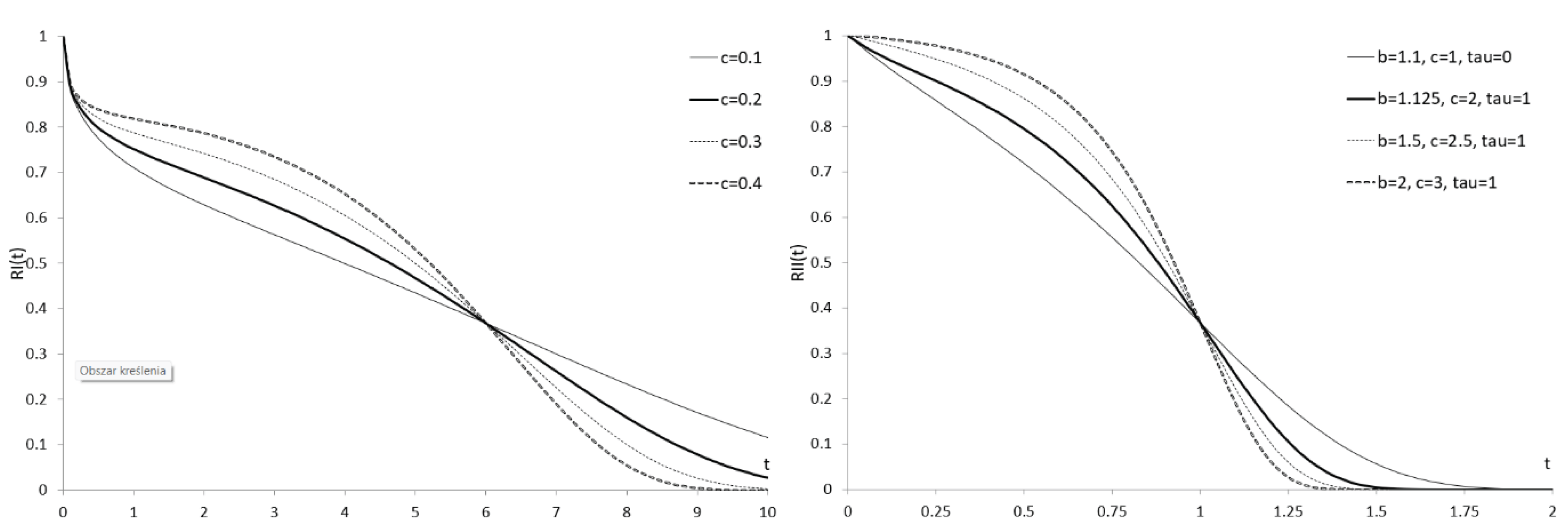
Figure 2.
FDF of the WDSFI with the parameter vector (left) and the FDF of WDSFII with the parameter vector (right).
Figure 2.
FDF of the WDSFI with the parameter vector (left) and the FDF of WDSFII with the parameter vector (right).
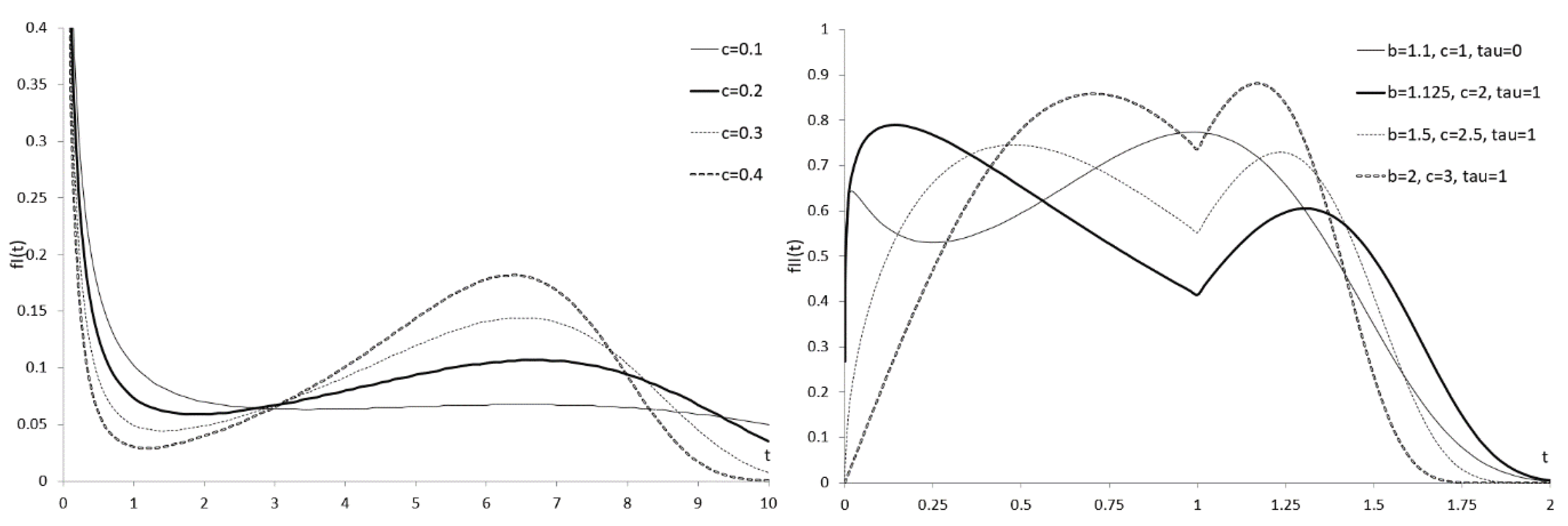
Figure 3.
HRF of the WDSFI with the parameter vector (left) and the HRF of WDSFII with the parameter vector (right).
Figure 3.
HRF of the WDSFI with the parameter vector (left) and the HRF of WDSFII with the parameter vector (right).

Figure 4.
HRAF of the WDSFI with the parameter vector (left) and the HRAF of WDSFII with the parameter vector (right).
Figure 4.
HRAF of the WDSFI with the parameter vector (left) and the HRAF of WDSFII with the parameter vector (right).
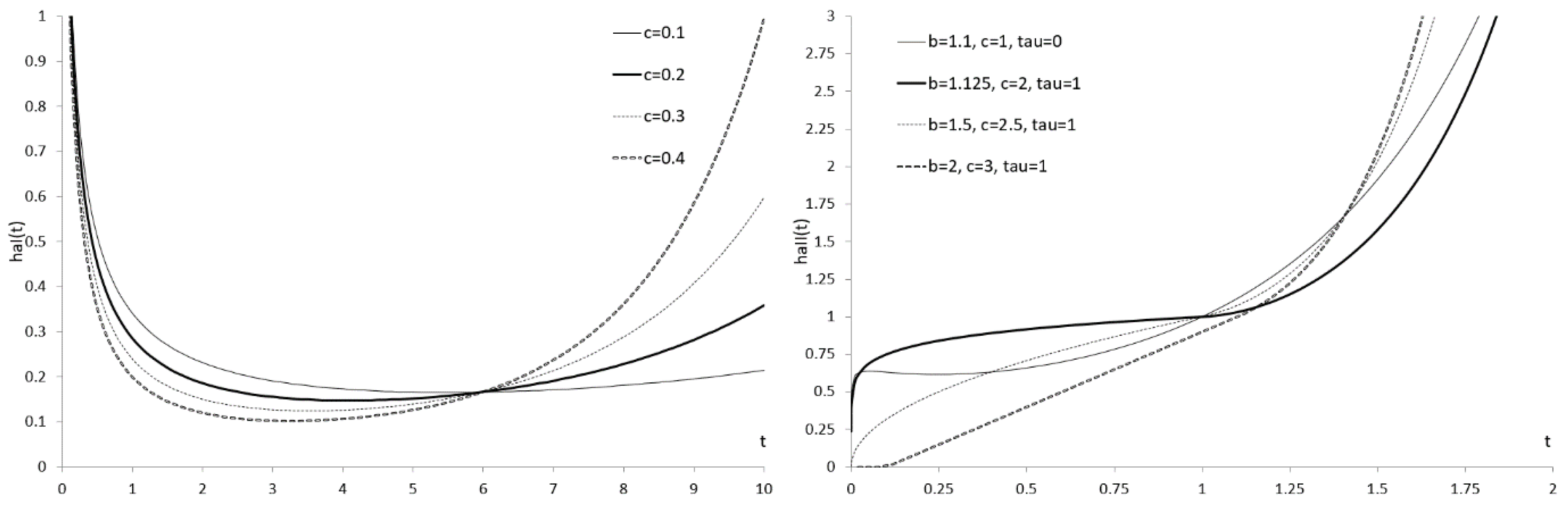
Figure 5.
Estimated FDFs for compared models for the failure times of devices
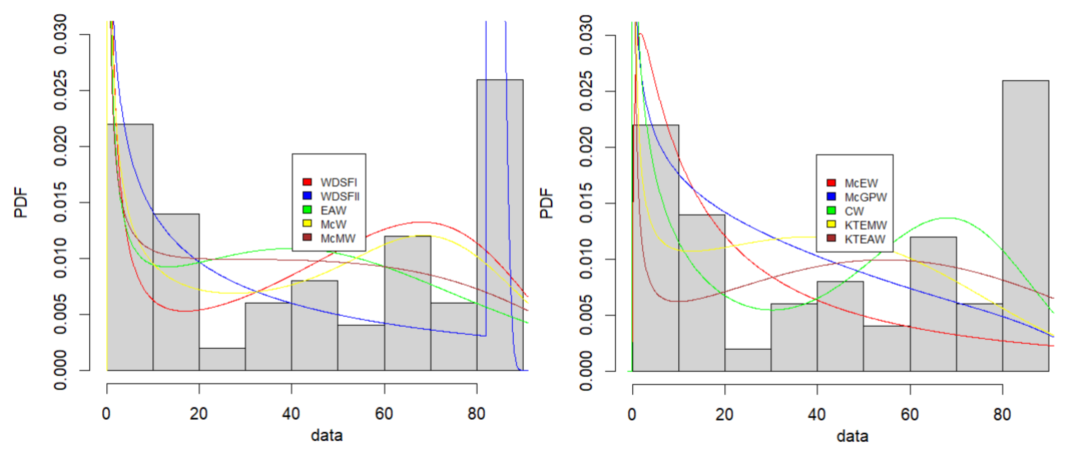
Figure 6.
Estimated PDFs for compared models for the times to the first failure of 500 MW generators
Figure 6.
Estimated PDFs for compared models for the times to the first failure of 500 MW generators
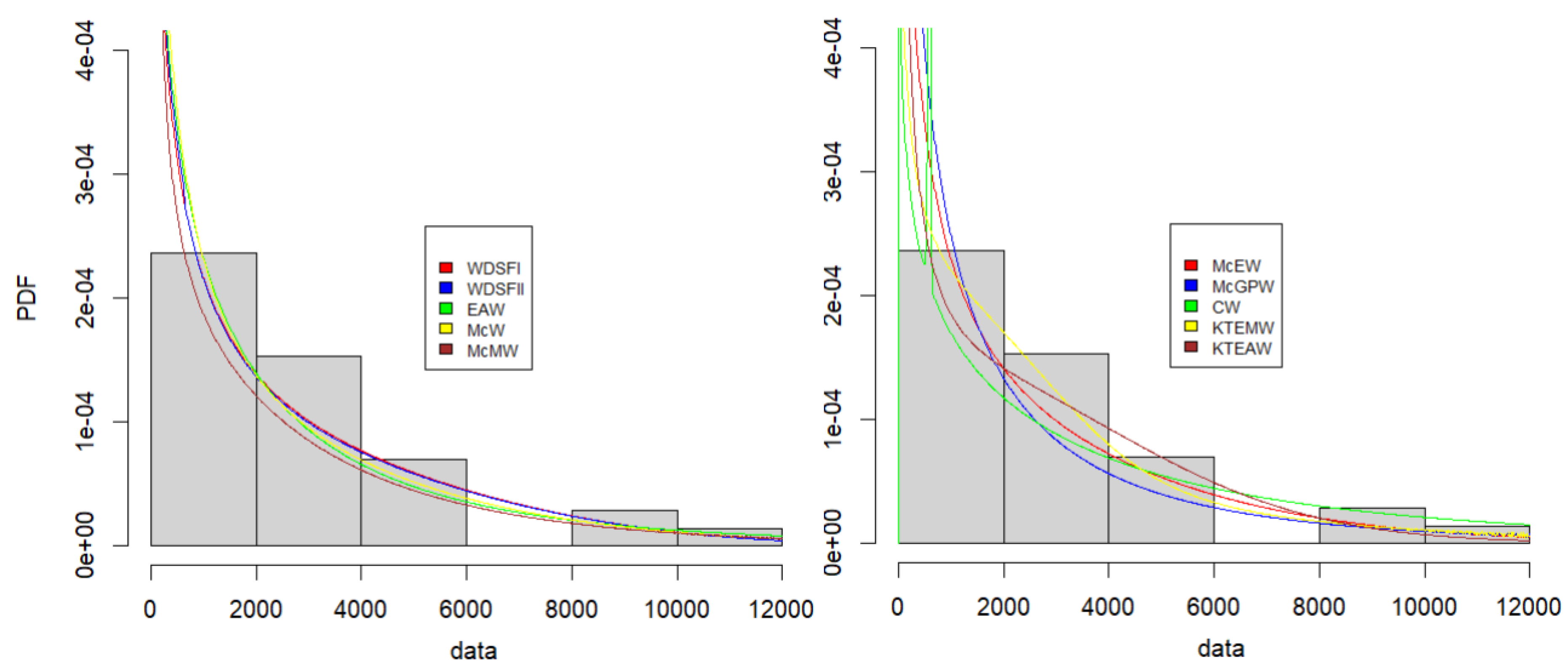

Table 1.
Standard deviation of scale parameter estimate for LTMs.
| LTM | a estimate |
|---|---|
| Exponential | 0.178 |
| Gamma | 0.242 |
| Weibull | 0.321 |
| Gamma Weibull | 0.937 |
Table 2.
Biases and RMSEs of the estimates obtained using various methods (M). Samples of size n were drawn from with .
Table 2.
Biases and RMSEs of the estimates obtained using various methods (M). Samples of size n were drawn from with .
| c | n | M | ||||||||
| BIAS | RMSE | BIAS | RMSE | BIAS | RMSE | BIAS | RMSE | |||
| 1 | 50 | ML | -0.0093 | 0.0847 | 0.1170 | 0.2658 | 0.0324 | 0.3247 | 0.1055 | 0.1508 |
| LS | 0.0018 | 0.0849 | 0.1184 | 0.2959 | 0.1120 | 0.5415 | 0.1571 | 0.2330 | ||
| WLS | 0.0013 | 0.0843 | 0.0908 | 0.2734 | 0.1270 | 0.5259 | 0.1392 | 0.2268 | ||
| LAW | -0.0024 | 0.0846 | 0.1552 | 0.3301 | 0.0306 | 0.4464 | 0.1663 | 0.2148 | ||
| 100 | ML | -0.0061 | 0.0575 | 0.0836 | 0.1886 | 0.0250 | 0.2409 | 0.0866 | 0.1342 | |
| LS | -0.0014 | 0.0555 | 0.1166 | 0.2270 | 0.0660 | 0.3680 | 0.1359 | 0.1974 | ||
| WLS | -0.0013 | 0.0550 | 0.0831 | 0.1934 | 0.0748 | 0.3380 | 0.1139 | 0.1807 | ||
| LAW | -0.0023 | 0.0558 | 0.1395 | 0.2562 | 0.0270 | 0.3430 | 0.1439 | 0.1884 | ||
| 200 | ML | -0.0009 | 0.0418 | 0.0594 | 0.1380 | 0.0249 | 0.1708 | 0.0721 | 0.1148 | |
| LS | 0.0012 | 0.0409 | 0.0949 | 0.1687 | 0.0435 | 0.2440 | 0.1122 | 0.1553 | ||
| WLS | 0.0012 | 0.0401 | 0.0636 | 0.1403 | 0.0516 | 0.2190 | 0.0888 | 0.1309 | ||
| LAW | 0.0019 | 0.0408 | 0.1103 | 0.1880 | 0.0269 | 0.2439 | 0.1285 | 0.1658 | ||
| 2 | 50 | ML | -0.0103 | 0.0558 | 0.1945 | 0.3719 | 0.0673 | 0.4724 | 0.0860 | 0.1267 |
| LS | -0.0101 | 0.0523 | 0.2871 | 0.5329 | 0.0708 | 0.8619 | 0.1339 | 0.1896 | ||
| WLS | -0.0080 | 0.0513 | 0.2265 | 0.4671 | 0.1225 | 0.7461 | 0.1221 | 0.1803 | ||
| LAW | -0.0075 | 0.0521 | 0.3303 | 0.5374 | 0.0576 | 0.7430 | 0.1544 | 0.1911 | ||
| 100 | ML | -0.0063 | 0.0423 | 0.1556 | 0.2762 | -0.0184 | 0.3740 | 0.0695 | 0.1095 | |
| LS | -0.0018 | 0.0385 | 0.2442 | 0.3704 | 0.0498 | 0.5900 | 0.1230 | 0.1606 | ||
| WLS | -0.0019 | 0.0380 | 0.1817 | 0.3139 | 0.0594 | 0.4483 | 0.0988 | 0.1331 | ||
| LAW | -0.0023 | 0.0385 | 0.2793 | 0.4055 | 0.0330 | 0.5268 | 0.1358 | 0.1660 | ||
| 200 | ML | -0.0045 | 0.0275 | 0.1127 | 0.2068 | -0.0101 | 0.2516 | 0.0556 | 0.0894 | |
| LS | -0.0016 | 0.0259 | 0.2165 | 0.2991 | 0.0407 | 0.3699 | 0.1142 | 0.1422 | ||
| WLS | -0.0015 | 0.0255 | 0.1521 | 0.2364 | 0.0500 | 0.3057 | 0.0869 | 0.1100 | ||
| LAW | -0.0016 | 0.0259 | 0.2533 | 0.3437 | 0.0294 | 0.3699 | 0.1292 | 0.1545 | ||
| 3 | 50 | ML | -0.0591 | 0.0561 | 0.2503 | 0.5285 | -0.1146 | 0.7230 | 0.0837 | 0.1741 |
| LS | 0.0025 | 0.0400 | 0.4460 | 0.7741 | -0.0951 | 1.1100 | 0.1307 | 0.1556 | ||
| WLS | 0.0022 | 0.0392 | 0.3795 | 0.6883 | -0.0782 | 0.9387 | 0.1040 | 0.1416 | ||
| LAW | 0.0027 | 0.0402 | 0.5165 | 0.8346 | -0.0772 | 1.0393 | 0.1456 | 0.1766 | ||
| 100 | ML | -0.0111 | 0.0493 | 0.1517 | 0.3145 | -0.1034 | 0.4895 | 0.0660 | 0.1184 | |
| LS | -0.0006 | 0.0288 | 0.3717 | 0.5462 | -0.0193 | 0.7243 | 0.1159 | 0.1485 | ||
| WLS | -0.0009 | 0.0284 | 0.2981 | 0.4545 | 0.0646 | 0.5678 | 0.1022 | 0.1290 | ||
| LAW | -0.0008 | 0.0290 | 0.4403 | 0.6089 | -0.0576 | 0.7586 | 0.1419 | 0.1721 | ||
| 200 | ML | -0.0078 | 0.0473 | 0.1212 | 0.2600 | -0.0650 | 0.3834 | 0.0409 | 0.0778 | |
| LS | -0.0003 | 0.0202 | 0.3340 | 0.4468 | 0.0154 | 0.4874 | 0.1099 | 0.1369 | ||
| WLS | -0.0004 | 0.0198 | 0.2655 | 0.3702 | 0.0496 | 0.3968 | 0.0941 | 0.1156 | ||
| LAW | -0.0003 | 0.0203 | 0.4135 | 0.5234 | 0.0335 | 0.5317 | 0.1381 | 0.1661 | ||
Table 3.
MLE, IC and KS values of models fitted to 50 failure times of devices.
| LTM | MLE | AIC | BIC | HQIC | KS | |||||||
|---|---|---|---|---|---|---|---|---|---|---|---|---|
| WDSFI | 63.296 | 0.591 | 0.026 | 448.826 | 454.562 | 451.011 | 0.133 | |||||
| WDSFII | 67.308 | 0.689 | 1.097 | 81.999 | 421.516 | 429.164 | 424.428 | 0.098 | ||||
| EAW | 3.660 | 0.046 | 0.002 | 1.571 | 107.658 | 469.737 | 479.297 | 473.377 | 0.154 | |||
| McW | 0.023 | 3.948 | 0.581 | 0.113 | 0.123 | 453.758 | 463.318 | 457.399 | 0.129 | |||
| McMW | 0.011 | 0.070 | 1.400 | 99.689 | 0.122 | 110.808 | 465.340 | 476.812 | 469.709 | 0.148 | ||
| McEW | 0.005 | 0.365 | 0.342 | 5.639 | 22.194 | 67.675 | 513.666 | 525.138 | 518.035 | 0.246 | ||
| McGPW | 0.004 | 0.975 | 3.756 | 30.574 | 0.026 | 43.588 | 473.988 | 485.460 | 478.357 | 0.269 | ||
| CW | 72.727 | 4.505 | 19.101 | 0.762 | 0.005 | 0.545 | 454.997 | 466.469 | 459.366 | 0.140 | ||
| KTEMW | 15.268 | 33.904 | 15.729 | 0.009 | 0.002 | 2.499 | 2.099 | 470.777 | 484.161 | 475.874 | 0.146 | |
| KTEAW | 0.092 | 1.608 | 0.0002 | 0.120 | 2.290 | 3.200 | 0.744 | 2.197 | 488.172 | 503.468 | 493.997 | 0.280 |
Table 4.
MLE, IC and KS values of models fitted to 36 times to the first failure of 500 MW generators.
Table 4.
MLE, IC and KS values of models fitted to 36 times to the first failure of 500 MW generators.
| LTM | MLE | AIC | BIC | HQIC | KS | |||||||
|---|---|---|---|---|---|---|---|---|---|---|---|---|
| WDSFI | 2615.140 | 0.725 | 0.00003 | 639.431 | 644.181 | 641.089 | 0.100 | |||||
| WDSFII | 2567.828 | 0.731 | 0.00003 | 644.846 | 641.410 | 647.744 | 643.621 | 0.100 | ||||
| EAW | 1.858 | 0.092 | 0.002 | 0.766 | 46.659 | 644.581 | 652.498 | 647.344 | 0.116 | |||
| McW | 0.016 | 0.212 | 64.343 | 7.5670 | 32.539 | 642.722 | 650.639 | 645.485 | 0.114 | |||
| McMW | 0.0007 | 0.068 | 3.047 | 4.772 | 8.793 | 0.386 | 652.555 | 662.056 | 655.871 | 0.175 | ||
| McEW | 0.073 | 0.371 | 21.007 | 0.104 | 0.126 | 23.577 | 645.083 | 654.584 | 648.399 | 0.109 | ||
| McGPW | 0.025 | 0.676 | 1.008 | 3.438 | 0.535 | 0.247 | 646.477 | 655.978 | 649.793 | 0.165 | ||
| CW | 4343.488 | 8.000 | 549.686 | 34.468 | 55.643 | 0.935 | 645.011 | 654.512 | 648.327 | 0.111 | ||
| KTEMW | 0.068 | 0.248 | 8.454 | 0.048 | 0.001 | 0.025 | 0.890 | 651.727 | 662.812 | 655.596 | 0.114 | |
| KTEAW | 0.923 | 1.417 | 3E-06 | 0.096 | 4.952 | 0.282 | 2.850 | 3.101 | 650.268 | 662.936 | 654.689 | 0.082 |
Disclaimer/Publisher’s Note: The statements, opinions and data contained in all publications are solely those of the individual author(s) and contributor(s) and not of MDPI and/or the editor(s). MDPI and/or the editor(s) disclaim responsibility for any injury to people or property resulting from any ideas, methods, instructions or products referred to in the content. |
© 2025 by the authors. Licensee MDPI, Basel, Switzerland. This article is an open access article distributed under the terms and conditions of the Creative Commons Attribution (CC BY) license (http://creativecommons.org/licenses/by/4.0/).
Copyright: This open access article is published under a Creative Commons CC BY 4.0 license, which permit the free download, distribution, and reuse, provided that the author and preprint are cited in any reuse.


