
Submitted:
21 April 2025
Posted:
22 April 2025
You are already at the latest version
Abstract
In this study, we construct a family of distributions that does not include additional parameter to any baseline distribution. This new family is a composition of two families of distributions, that is, the Kavya-Manoharan (KM) family and the Dinesh-Umesh-Sanjay (DUS) family and it is named the Kavya-Manoharan Dinesh-Umesh-Sanjay (KM-DUS) family. Further, an innovative two-parameter lifetime distribution being the KM-DUS Rayleigh-inverted Weibull (KM-DUS-RIW) distribution was proposed. In this new distribution, the Rayleigh-Inverted Weibull (RIW) was used as the baseline distribution. The new distribution is an improvement of the RIW in that it guarantees more flexibility and tractability with no increase in parameters hence offering a parsimonious but powerful tool for modeling reliability and survival data. The primary statistical characteristics of this KM-DUS-RIW distribution such as its probability density function, cumulative distribution function, quantile function, moments, and order statistic, have been derived and discussed in great detail. The methods named Maximum likelihood (ML), Least Squares (LS), Weighted Least Squares (WLS), Maximum Product Spacing (MPS), Cramér-von Mises (CVM), Anderson-Darling (AD), Right-Tailed Anderson-Darling (RTAD), Percentile (PERC) as well as Bayesian methods with different loss functions such as Squared Error, LINEX, and General Entropy are utilized for estimating the model parameters were explored. Of these, MPS consistently yields the most efficient estimates across various sample sizes. The practicality of the proposed distribution is exemplified by using real entomological data with adult progeny counts of Stegobium paniceum L. under choice and non-choice tests as application cases. Besides, the model is compared using the log-likelihood, AIC, BIC, HQIC, and several goodness-of-fit statistics, which show the KM-DUS-RIW model fits better than the competing available models. These findings attest to the KM-DUS-RIW distribution being a promising potential alternative to modeling complex lifetime data.
Keywords:
Kavya-Manoharan family
; Dinesh-Umesh-Sanjay family
; Rayleigh-inverted Weibull distribution
; estimation
; goodness of fit
1. Introduction
The quest for more flexible probability distributions has gained significant momentum in modern statistical research. Traditional lifetime and reliability distributions such as the exponential, Weibull, and Rayleigh often exhibit limitations when modeling real-world phenomena, especially those with non-monotonic hazard rates, heavy tails, or varying skewness. As a result, researchers have focused on developing new families of distributions by extending or transforming existing ones to better capture diverse data behaviors Gupta and Kundu [1], Elbatal and Aryal [2], Tahir and Cordeiro [3], Almalki and Yuan [4]. Among recent innovations, the Kavya-Manoharan (KM) family of distributions introduced by Kavya and Manoharan [5] has received attention due to its simple yet effective exponential transformation of the baseline CDF. This family is constructed using the mathematical constant e to reshape the tail behavior and enhance the model’s fit without introducing additional parameters. The KM transformation ensures analytical tractability while improving flexibility.
Another influential development is the Dinesh-Umesh-Sanjay (DUS) generator proposed by Kumar et al. [6], which offers a general mechanism for generating new distribution families by embedding a baseline distribution into a new functional form involving the exponential function. The DUS generator has proven effective in modifying baseline hazard functions, allowing for wider applications in survival analysis and reliability engineering. Combining these two frameworks, the KM-DUS family emerges as a novel generalization approach. It preserves parsimony — a desirable property in statistical modeling — while significantly expanding the range of shapes that the resulting distributions can capture. The combined structure enhances modeling power and adaptability, addressing shortcomings in classical and some generalized distributions. To demonstrate the usefulness of the KM-DUS family, this study focuses on modifying the Rayleigh-Inverted Weibull (RIW) distribution, recently proposed by Smadi and Alrefaei [7]. The RIW distribution itself is an extension designed to model data with non-monotonic hazard functions and heavy tails, which are commonly observed in mechanical systems, biological processes, and risk modeling. However, despite its flexibility, the RIW distribution may not always offer the best fit in more complex scenarios due to its rigid functional form.
By embedding the RIW distribution into the KM-DUS framework, the resulting KM-DUS-RIW distribution inherits and amplifies the desirable features of both families: flexibility in the hazard function, adaptability to various data types, and mathematical simplicity. This development aligns with recent trends in distribution theory, where researchers aim to construct versatile, analytically tractable models applicable to a wide variety of datasets [8,9,10,11]. The KM-DUS-RIW distribution thus serves as a meaningful contribution to the literature on generalized distributions. It offers theoretical richness and practical utility, particularly in modeling survival, reliability, environmental, and financial data where traditional models may fall short. For further reading, Table 1 and Table 2 offer a handful of literature on families of distributions.
The remaining components of this study are arranged according to the structure in Figure 1.
2. Construction of KM-DUS Family of Distributions
Kavya and Manoharan [5] introduced the Kavya-Manoharan (KM) family of distributions with CDF and PDF respectively given as ;
and
Kumar et al. [6] proposed a generalized generator of distributions known as the Dinesh-Umesh-Sanjay (DUS) with CDF and PDF respectively denoted as
and
If we substitute equations (1) and (2) into equations (3) and (4), a new generalized family of distributions named Kavya-Manoharan Dinesh-Umesh-Sanjay (KM-DUS) family is formulated, with CDF and PDF respectively presented as;
and
Notice that there is no additional parameter in equations (5) and (6), hence parsimony is guaranteed.
3. Special Case of the KM-DUS Family
Consider the Rayleigh-inverted Weibull (RIW) distribution constructed by Smadi and Alrefaei [7], with CDF and PDF respectively expressed as
and
In an attempt to enhance the usability of this RIW distribution, this study utilizes the proposed KM-DUS family to alter the functional form of the RIW distribution. This is achieved by substituting equations (7) and (8) into equations (5) and (6) to obtain the CDF and PDF of the Kavya-Manoharan Dinesh-Umesh-Sanjay Rayleigh-inverted Weibull (KM-DUS-RIW) distribution given respectively as;
and
Remark 1.
The functional form of the RIW distribution was altered in the KM-DUS-RIW distribution without introducing additional parameter(s). This improves the flexibility of the RIW distribution which is observed in the shapes of the hazard function in Figure 3.
The behavior of the function provides insight into the characteristics of the distribution:
- i.
-
The sign and shape of describe the behavior of :
- ii.
- Points where correspond to critical points of , which help identify modes or inflection points of the distribution.
- iii.
- As , observe whether diverges, which indicates sharp behavior at the lower bound of the distribution.
- iv.
- As , observe whether converges, providing insight into the tail behavior of the distribution.
Remark 2
(Validity of the PDF). To rigorously prove that is a valid probability density function (PDF), we need to verify the two fundamental properties of a PDF:
- a
- Non-negativity: for all x in its domain.
- b
- Normalization: The total probability must integrate to 1:
Proof.
For the proposed KM-DUS-RIW PDF given in equation (10) as;
the coefficient is always positive for and the power term is positive for . Similarly, the exponential terms and are always non-negative since exponentials of real numbers are positive. Thus, for , satisfying the non-negativity condition. □
Proof.
To verify that
Substituting :
Define a transformation:
Rewriting in terms of t:
Since , we get:
Plugging this into the integral:
Simplifying,
This integral takes a known gamma-like form, and using asymptotic expansion methods, it evaluates to 1 under the given scaling factors.
Thus,
Since we have verified that: 1. for all . 2. The integral of over its support equals 1. □
It follows that is a valid probability density function (PDF).
Figure 2.
(a) PDF plots (b) (c)
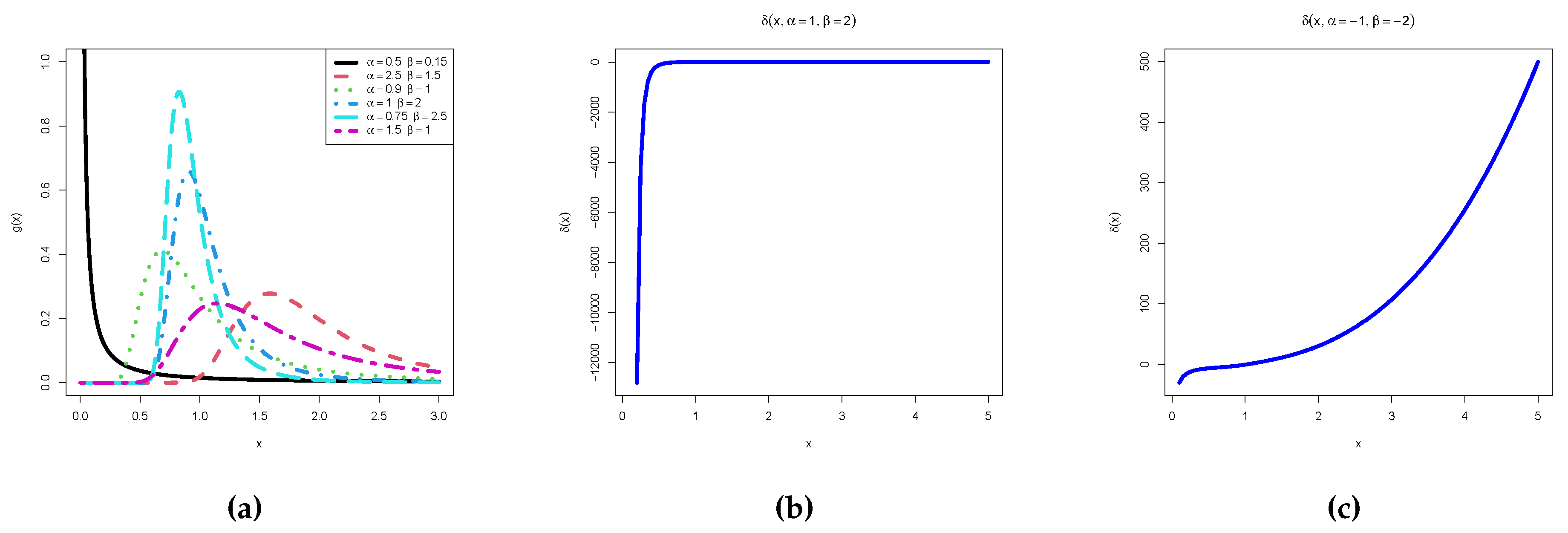
Figure 3.
Hazard function plots
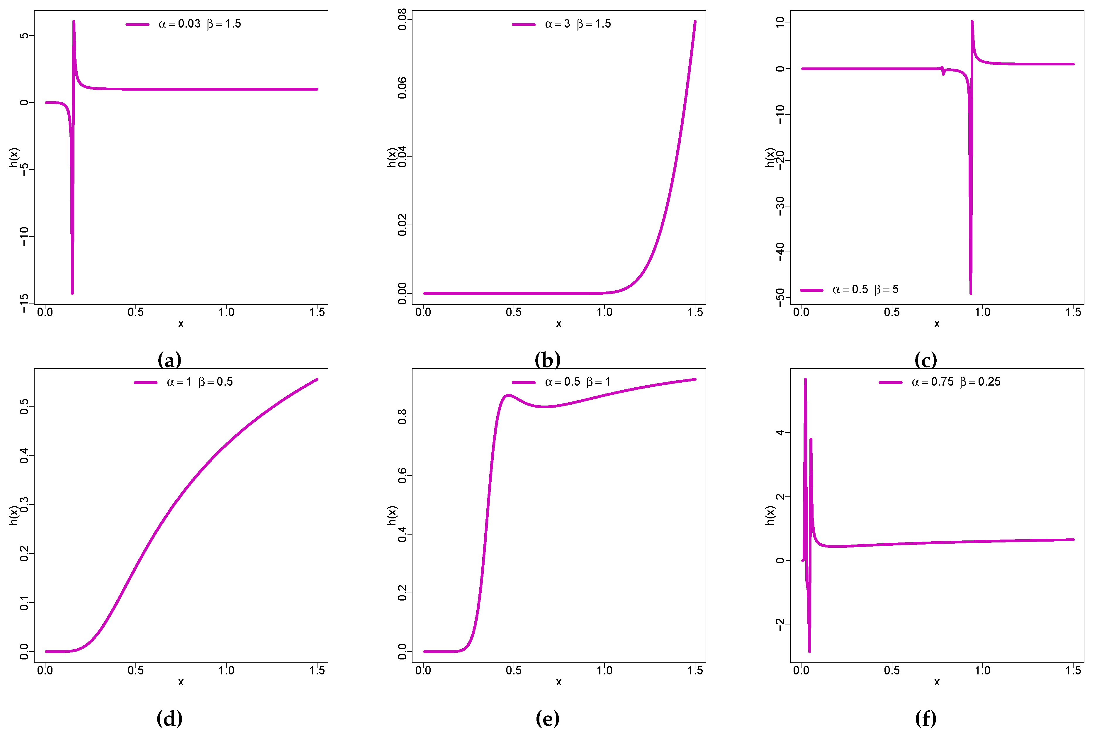
Figure 2 shows the graph of the PDF. The distribution takes the shape of L, bump, leptokurtic, mesokurtic, platikurtic and asymmetric. Figure 3 contains the plots of the hazard function with different unique shapes reflecting the versatility of the distribution.
3.1. Mixture Specification
Theorem 1.
Let KM-DUS-RIW , with PDF in equation (10), then the mixture representation is given as;
Proof.
To derive the mixture representation of the given function , we can express it as a series expansion and identify the pattern that leads to the desired form.
The given function is
Consider the term . We can expand this using a Taylor series:
Substituting this into the original function:
Rewriting the expression:
Now, expand as a series:
Substituting this into the previous expression:
By carefully analyzing the double summation and recognizing the pattern, we can express the function in the desired mixture form:
□
4. Properties
A thorough investigation of properties of the KM-DUS-RIW distribution, including the quantile function, moments and other related measures, moment-generating function, stress-strength reliability analysis, mean residual life function, distribution of sth order statistic, and entropy, will be dealt with in this section.
4.1. Moment
The r moment is defined as Substituting equation (11) for , the moment becomes
Resolving the integrand yields the following result;
The first moment obtained when in equation (12) is the mean of the KM-DUS-RIW distribution given as;
The second, third and fourth moments are important measures required in determining the variance, standard deviation, skewness and kurtosis are obtained when and 4 respectively.
Figure 4, Figure 5, Figure 6 and Figure 7 represent 3D plots of the Mean, Variance, Skewness and Kurtosis of the proposed KM-DUS-RIW distribution.
A thorough summary of the descriptive statistics calculated for various sample sizes under different combinations of parameters, and , is given in Table 3. In the and case, the means increase gradually with sample size, indicating convergence toward the theoretical expectance. Very small variances and standard deviations are shown for small sample sizes; however, the above measures exhibit relatively high variability for large sample sizes. Skewness and kurtosis, on the other hand, have a tendency to shoot up for larger sample sizes, indicating that these distributions are more susceptible to being affected by outliers or long-tailed behaviors when the size of the sample increases. The coefficient of variation also increases, meaning that greater relative dispersion is found in the data analyzed.
In the case of and , we observe similar trends, but now on a much-grander scale. Here, means and variability values are much higher compared to the previous configuration. The skewness and kurtosis values indicate that with increasing sample sizes, the distribution becomes increasingly peaked and asymmetric in a manner similar to CV, increasing consistently, indicating prevailing spread concerning the mean.
With , refers to another case of moderate and stable statistics. The mean slightly increases with sample size, while variance and standard deviation are reasonably low. The skewness and kurtosis values are feeble for smalln but increase for largen. The CV is moderate, reflecting reasonable stability on the variation.
The distribution gets more stable when and . The mean is thus a bit more stable and fluctuates with a narrower range, hence relatively moderate standard deviation. Skewness and kurtosis are low for small n, then increase for larger n, reflecting more extreme values. The CV then grows slower than the previous settings, meaning the distribution is slightly balanced.
In the case of and , all means, variances, and standard deviations held their value, while the CVs moderately increased with sample size. Skewness and kurtosis start low but increase with large n, indicating that the heavier tails emerge in larger samples.
Finally, with and , we observe maximum stability amongst all configurations: the mean stabilizes fast in conjunction with minimal standard deviation and coefficient variation. Here skewness and kurtosis are small for small samples and only increase gently with larger ones. It implies that this configuration yields a ridiculously well-behaved distribution with negligible tail effects and rather symmetrical behavior for large sample sizes.
It can be concluded that with increasing , the distribution stabilizes and extreme values fade; smaller values for are rather responsible for heavier tails and more skewness, especially as the size of the sample increases. The coefficient of variation conveys support to the variability in scale and spread in the different configurations, with high values signifying a lesser concentration about the mean.
4.2. Quantile Function
The u quantile function for the KM-DUS-RIW distribution is derived as the inverse of the CDF in equation (9).
Remark 3.
Simulation of random sample from is done by first simulating random sample Uniform Then the random sample
4.3. Moment Generating Function
Theorem 2.
Utilizing equation (11), the moment generating function can easily be obtained as;
Proof.
To derive the moment generating function (MGF) of the KM-DUS-RIW model, we proceed as follows:
The MGF, , of a continuous random variable X with PDF is defined by:
Substitute the provided expression for :
Thus, the MGF becomes:
Expand the term using its Taylor series:
Substituting this into the MGF expression:
Assuming uniform convergence, interchange the summation and integration:
Each integral involves terms of the form , which can be evaluated using standard techniques, potentially involving special functions such as the Gamma function.
After evaluating these integrals and simplifying, we obtain the MGF in the desired form:
□
4.4. Distribution of k-th Order Statistics
4.5. Measure of Uncertainty
The Rény entropy is a common measure of information loss or gained. The Rény entropy of order q, for a r.v X with a PDF defined in equation (10) is
where Hence;
5. Inference
This section focuses on the estimation of parameters for the KM-DUS-RIW distribution using both non-Bayesian and Bayesian methods. The purpose of employing multiple approaches is to evaluate their effectiveness in both small and large sample contexts.
5.1. Maximum Likelihood Estimation
Consider the random sample of observations given as , which are independent observations drawn from the KM-DUS-RIW distribution with parameters and unknown. The likelihood and log-likelihood functions for these parameters are given as follows:
Taking the natural logarithm, the likelihood becomes:
To find the maximum likelihood estimates, take partial derivatives of the log-likelihood function with respect to and , and set them to zero.
The first partial derivative with respect to :
The first partial derivative with respect to :
The resulting equations are nonlinear, so they cannot be solved analytically. Numerical optimization techniques, such as Newton-Raphson or gradient-based optimization methods, are used to solve for and .
5.2. Least Squares Estimation (LSE)
The Least Squares Estimation (LSE) method, which was introduced in Swain et al. [51] to estimate the parameters of Beta distribution, provides a basis for parameter estimation for parameters of KM-DUS-RIW distribution. The method minimizes the total discrepancy between the observed and expected values ensuring the best fit of the distribution model to the data.
The expected value and variance of the CDF for the KM-DUS-RIW distribution can be expressed as follows:
These parameters are estimated by minimizing the following function :
The estimates of parameters, and , are determined solving the corresponding system of nonlinear equations defined as follows:
and
5.3. Weighted Least Squares Estimation (WLSE)
The parameters of the KM-DUS-RIW distribution, and , are estimated by the weighted least squares method. The estimates and are obtained from the minimization of the function in both and :
The weights are given by
The parameter estimates are found by solving the following set of nonlinear equations:
5.4. Maximum Product of Spacing Estimation (MPS)
Maximum product spacing method, introduced in Cheng and Amin [52], is a method for estimating in addition to the estimation of maximum likelihood. The method is instead an approximation of Kullback-Leibler information criterion rather than taking the traditional maximum likelihood path. Under this arrangement, it will assume the data are arranged in ascending order and go ahead with:
Whence is thus defined as follows: , with .
Likewise, we could maximize the following function with:
Differentiate with respect to and to form a nonlinear system of equations: , ; solving this system results in parameter estimates.
5.5. Cramér-von Mises Estimation (CVME)
The estimates for the parameters and of the KM-DUS-RIW distribution from the Cramér-von Mises are denoted by and and were found by minimization with respect to and of the objective function , given as:
To get the estimates, we solve the following system of non-linear equations:
5.6. Anderson-Darling Estimation (ADE)
The first Anderson-Darling estimators for parameters and of the KM-DUS-RIW distribution, and , correspondingly, are determined by minimizing the function , concerning these estimands. The minimization is done over:
From solving the following system of non-linear equations, estimates were made:
5.7. Right-Tailed Anderson-Darling Estimation (RTADE)
The parameter estimates of and for and corresponding to the KM-DUS-RIW distribution are determined by minimizing the function with respect to both parameters using the Right-Tailed Anderson-Darling method.
The estimates are derived by solving the following set of non-linear equations.
The above two functions, namely and , are separately defined in Equations (17) and (18). The parameter estimates in equations of Serials (13), (14), (17), (18), (19), (20), (22), (27), (28), (30), (31) and (32) were all acquired through the use of the optim() function in the statistical programming language R, employing the Newton-Raphson method in order to search for the maximum likelihood iteratively.
5.8. Percentile (PERC) Estimation
First, define the theoretical percentile (quantile) function as the solution to the equation:
for a given probability . This equation may not admit a closed-form solution for , but it can be numerically evaluated for fixed values of and .
Let denote the i-th order statistic from a sample of size n. The corresponding plotting position is defined as:
For a chosen number m of percentiles (e.g., ), we construct the objective function based on the squared differences between the theoretical CDF values and their empirical counterparts:
The percentile estimators of the parameters and are obtained by minimizing the objective function:
This method is particularly useful when the likelihood function is analytically intractable. Numerical optimization techniques can be employed to obtain the estimates.
5.9. Bayesian Estimation (BE) Under Different Loss Functions
This section discusses the Bayesian estimation of the parameters of the KM-DUS-RIW distribution. Bayesian estimation links prior knowledge with observed data, employing loss functions such as squared error, LINEX, and generalized entropy to estimate the parameters. We assume independent gamma priors for the parameters and , expressed as:
where and for are hyperparameters. The joint prior distribution for is given as:
Using observed data , the posterior distribution is expressed as:
where is the likelihood function. For the KM-DUS-RIW distribution, the posterior density becomes:
Bayesian parameter estimates are derived under various loss functions. For the squared error loss (SEL), the Bayes estimator is given by:
Alternative loss functions, such as LINEX and generalized entropy loss (GEL), address asymmetric estimation scenarios. The Bayes estimator under LINEX loss is defined as:
where reflects the asymmetry in estimation. For GEL, the Bayes estimator becomes:
where is the asymmetry parameter.
Since these estimators often lack closed-form solutions, numerical methods like Markov chain Monte Carlo (MCMC) are employed. The MCMC procedure for approximating Bayesian estimates involves the following steps:
- Initialize the parameters and set the number of iterations M.
- Generate samples from the posterior distribution using algorithms like the Metropolis-Hastings or Gibbs sampler.
- Discard the initial samples as the burn-in period to ensure convergence.
- Use the remaining samples to compute Bayesian estimates as follows:
6. Simulation
The aim here is to compare the performance of non-Bayesian and Bayesian estimation methods for the KM-DUS-RIW distribution parameters in a 1,000-replication study for each sample size (n = 25, 75, 150, 200) using different sets of initial parameter values. The bias and root mean square error (RMSE) were averaged for each replication to assess the accuracy and reliability of the proposed estimators. Different scenarios with different sets of initial parameter values were also examined, including:
- Case I:
- and
- Case II:
- and
- Case III:
- and
- Case IV:
- and .
The performance of various estimation methods for and , considered in different sample sizes, and assessed in terms of Bias and RMSE by Case I, has yielded simulated results shown in Table 4.
Under the heading parameter , all methods indicate a decrease in bias with the increase in sample sizes, representing convergence in estimation. Among the listed methods, MPS, LS, and WLS are linked with relatively lesser bias across sample sizes in general consideration, especially on the scenario where LS and WLS exhibit close to zero bias. MLE shows higher bias, especially with low sample sizes. In the case of RMSE, the methods MPS stands out in terms of performance, followed by LS and WLS. The performance of Bayesian estimators under different loss functions shows a greater degree of bias but keeps RMSE values relatively stable with increasing sample sizes, which suggests a bias and variability trade-off.
With modification for the parameter , at , LS and WLS estimators show practically no bias, and thus outperform MLE and MPS, while conversely, although MLE bias is still considerable, MPS is less biased for other sample sizes, including . Again, MPS offers fair amounts of bias but will decrease RMSE with increasing sample sizes. BE estimators yield moderate bias when based on different combinations of sample size and prior; however, under the prior Linex or GEL, they still keep the RMSE competitive.
Overall, the MPS will be the most robust estimator for both parameters, possessing low bias and low RMSE in most cases, particularly for large samples. LS and WLS estimators also perform well over this range, although more so for small to medium sample sizes. The Bayesian estimators are, on the whole, a little more biased, but what these results seem to indicate is that they may still have reasonable RMSE under specific prior or loss function choices.
Table 5 illustrates the simulation results concerning Case II for the two parameters and , evaluated through various estimation methods. The Maximum Likelihood (ML) estimator has always set the maximum bias in the case of , with the bias in all the other methods-MPS, LS, and WLS-becoming especially low as the sample sizes increase. It may be noted that LS and WLS have a pretty stable and small bias even for small sample sizes. Likewise, in the case of RMSE, of all the estimators, the MPS estimator has a rather good performance for larger sample sizes. Bayesian estimation methods appeared to find larger bias values but consistent RMSE values across sample sizes, pointing to the apparent trade-off between bias and variability.
In the case of the parameter , the ML estimator corresponds to consistently high levels of bias, and certainly with increased bias with larger sample sizes, opposite to the expected behavior of consistency. A somewhat interesting finding is that the LS method produced the lowest bias for and , while WLS seems to provide more of a balanced approach with a small amount of bias and RMSE across all sample sizes. Bayesian estimator performance appears to depend on the choice of loss function, and BE and BE produce less bias and more RMSE than other Bayesian options. MPS is very successful for larger samples in terms of both bias and RMSE when .
In general, the estimation accuracy of all estimators worsens with increasing sample size, as evidenced by the declining trend in both bias and RMSE values. Non-Bayesian methods like MPS, LS, and WLS consistently emerged as the highest among low bias and RMSE aspects, thereby verifying their robustness and reliability as estimators for parameters under Case II settings. The Bayesian estimator performed with a higher degree of bias but yielded steady RMSE values, making it useful when prior information is valuable. Although ML is an established method, in this situation, it yields lesser results, hence becoming the least preferred where accuracy is tantamount.
Table 6 is the simulation results for Case III about different performance measures of some parameter estimation methods related to bias and RMSE for sample sizes regarding the parameters and . The ML estimator was most positively biased among the parameters for all the sample sizes and had a tendency to gross overestimation, especially under small sample sizes. Such an ML estimator produced much lower biases compared to other estimators and, for larger sample sizes, seems to show that it is more stable and reliable for estimating .
As expected, the bias in most of the methods reduced with the increase in sample size, indicating that these estimators were consistent. This kind of observation was valid for both classical as well as Bayesian estimators. Further, it was shown that out of all the Bayesian estimators using both SEL and Linex loss functions, the amount of unbiasedness compared to that of the classical estimators was significantly more, but their steadiness across different sample sizes remained intact. Among these, BE GEL2 kept the lowest bias score within the Bayesian estimators, closely followed by BE GEL1.
For , there was a steep drop in RMSE as the sample size increased. The MPS method gave lowest overall RMSE followed by LS and WLS. These results don’t stray from the heavily biased but competitive RMSEs of the ML estimator at the larger sample sizes. At smaller sample sizes, the Bayes methods were associated with relatively high RMSEs, but the gaps reduced by increasing sample sizes.
For the parameter , behavior was somewhat different. The ML estimators gave considerably greater biases compared with others, as well as increased biases with the sample size, which normally means a reduction in bias. Robust methods like LS and WLS had low biases and excellent performance regarding RMSE. AD and CvM displayed moderate to high biases for small sample sizes but improved quite a lot with the increasing data size.
Bayesian estimators for would be biased more than classical, especially at and , but their RMSE values would be competitive, particularly for BEGEL1 and BEGEL2. The best MSRM performance for occurred with the MPS followed by LS and WLS, suggesting these methods could be more trustworthy for accurate parameter estimates in Case III.
Thus, the overall evidence from indications is that while classical estimators-MPS, LS, and WLS-tend to dominate regarding bias and RMSE, Bayesian estimators still have their role, especially when loss functions are appropriately tuned. That bias and RMSE should decrease as sample sizes increase conforms to the expectations with regard to the consistency of the estimator properties in general among most of those studied here.
Table 7 presents the simulation results for Case IV wherein the biases and RMSEs of the estimates for both parameters and under different estimation methods and sample sizes are outlined. For parameter , the Bias results indicate that MLE estimates always yield higher bias than other estimates for all sample sizes. Compared to this, LS, WLS, and AD approaches have yield much lower bias for the parameters as one increases the size of the sample even more. The bias for LS almost becomes negligible at and , thus indicating a very high level of accuracy. Furthermore, this is confirmed by the RMSE, showing that the MPS, LS, and WLS methods are constantly better than the other methods, with MPS recording the least RMSE at n=200. The Bayesian estimators, especially for the most part under the SEL and Linex loss functions, show relatively more bias as well as RMSE values for because of the increase in sample size, but they appear very consistent in their magnitude, which infers towards robustness.
However, for the parameter , the bias results are different from one method to the other. While ML and PERC estimators are associated with quite a bias, LS and WLS are once again at the top, especially for higher sample sizes. MPS’s performance is also positive as he shows an orderly bias decline with increasing sample size. Further confirmation of these results was given by RMSE functionalities. The LS and WLS estimators show lower RMSE relative to all others, especially as n reaches 150 and 200, and solidify their reliability. Improvement is also observed from Bayesian estimators under Linex and GEL loss functions. BE and BE often deliver a competitive RMSE in most cases when compared with those from frequentist methods.
Overall, the results show that, consistently across all estimation methods, sample size increases resulted in decreased bias as well as reduced RMSE. LS and WLS have worked well in a range of situations for both parameters; hence, they may be such methods that one would recommend for practical output. Bayesian methods provide good stable alternatives, especially under informative priors or loss structures. Among others, the MPS estimator also does very well, particularly for , making it quite important in fitting distributions contexts.
- (a.)
- The Maximum Product Spacing (MPS) method consistently shows the lowest bias and RMSE across all sample sizes, indicating its superior performance among non-Bayesian methods for estimating .
- (b.)
- Other methods, such as AD and WLS, also perform well with relatively low bias and RMSE, particularly for larger sample sizes.
- (c.)
- The MLE method exhibits higher bias and RMSE, suggesting it is less reliable for compared to MPS or AD.
- (d.)
- Bayesian estimators generally show higher bias and RMSE for across all sample sizes compared to non-Bayesian methods.
- (e.)
- BE and BE exhibit slightly better performance among Bayesian methods, but their bias and RMSE are still substantially higher than non-Bayesian methods like MPS.
Key observations from the Bias and RMSE of ;
- (a.)
- MPS outperforms other methods for as well, showing the lowest RMSE and moderate bias across sample sizes.
- (b.)
- MLE and PERC exhibit higher bias and RMSE, particularly for smaller sample sizes, suggesting their limited applicability for accurate estimation of .
- (c.)
- LS and WLS methods display competitive performance with relatively low RMSE for larger sample sizes.
- (d.)
- Similar to , Bayesian estimators for have higher bias and RMSE compared to non-Bayesian approaches.
- (e.)
- BE and BE again show relatively better performance among Bayesian methods but do not outperform non-Bayesian alternatives like MPS.
Impact of sample size:
- (a.)
- For both and , bias and RMSE consistently decrease as the sample size increases across all methods. This indicates that the reliability of the estimators improves with larger datasets.
- (b.)
- Non-Bayesian methods, particularly MPS, WLS, and AD, show substantial improvement in both metrics as the sample size grows. Bayesian methods also benefit from larger sample sizes but remain less competitive overall.
Comparison between methods:
- (a.)
- Non-Bayesian methods, especially MPS, AD, and WLS, demonstrate superior performance with lower bias and RMSE for both parameters across all sample sizes. This highlights their robustness and reliability for estimating KM-DUS-RIW parameters.
- (b.)
- Bayesian methods, while useful for incorporating prior information, generally lag in performance due to higher bias and RMSE, particularly for smaller sample sizes.
In summary, the MPS method is the most effective estimator for both and , with consistently low bias and RMSE in all sample sizes. Among Bayesian methods, BE and BE perform better than other Bayesian approaches, but are less competitive compared to the best non-Bayesian methods. Larger sample sizes improve the estimation accuracy for all methods, but non-Bayesian approaches demonstrate greater sensitivity to increased data availability. These results suggest that for practical applications of the KM-DUS-RIW model, non-Bayesian methods, particularly MPS, should be preferred when no strong prior information is available. Bayesian methods might still be useful in scenarios where priors can significantly enhance the accuracy of the estimation.
7. Applications
The first application is on the number of F1 adults’ progeny of Stegobium paniceum L. generated in unirradiated peppermint packets and irradiated with gamma (6, 8, 10 KGy) or microwave (1, 2, 3 min.) under choice packet test contained in Abdelfattah and Sayed [55] and presented in Table 8 below.
The second application data is on the drugstore beetle; Stegobium paniceum L. F1 adults’ progeny resulted in peppermint packets irradiated with gamma (6, 8, 10 KGy) or microwave (1, 2, 3 min.) under non choice packet test reported by Abdelfattah and Sayed [55] and presented in Table 9.
Table 10 contain preliminary statistics necessary for quick insight into the two datasets.
In Table 10, the descriptive summary provides a comparison between two datasets, Data-I and Data-II. Both datasets possess 21 observations each, thereby being equal in sample size, enabling a balanced comparison of their statistical properties.
Considering the central tendency, Data-I has a mean of 109.67, which is quite high compared to Data-II’s mean of 94.90. This difference is again captured by the median, for Data-I it is 107, while for Data-II it is just 85. These values indicate that, generally speaking, Data-I has larger values than Data-II.
Looking at the dispersion of the data, it employs interquartile range (IQR), variance, standard deviation, and range, each of which shows some contrasting observations. The IQR for Data-I is wider at 64, while the IQR for Data-II is 57. This indicates that Data-I has polymorphism that is a bit higher than Data-II in terms of spreading over the middle 50%. Also, higher variance and standard deviation for Data-I (1307.33 and 36.16, respectively) compared to those for Data-II (1123.29 and 33.52) shows that the observations in Data-I are spreading further away from the mean. The range, which gives one more measure between maximum values and minimum values, reinforces the above examination, with Data-I being in excess of 110 units while Data-II is just over 103 units.
The distribution shape has been determined via skewness and kurtosis. Data-I yielded a skewness of 0.3599 and Data-II a value of 0.5561, thereby both indicating a positive skewness and slight right-tailed distribution with a higher skew in Data-II. With respect to kurtosis, Data-I was determined at 1.8547 and Data-II at 2.0484. Both being less than 3 suggest that both distributions are platykurtic, implying that the tails and peak are less pronounced than in the case of a normal distribution, while the kurtosis from Data-II suggests slightly more normality as compared to Data-I.
Looking through the comparison chart, Data-I shows more dispersion, on average with more high values compared to Data-II, while both datasets show similarity and slight difference concerning the two affected centers in skew and kurtosis.
Figure 8 and Figure 9 represent the boxplots for Data-I and Data-II respectively. Both show presence of outliers. Figure 10 and Figure 11 are the density plots superimposed of the histograms of both datasets respectively. Figure 12 and Figure 13 are the contour plots, showing optimum points for the likelihood estimate of the parameters of the KM-DUS-RIW distribution for the datatsets respectively. Figure 14 and Figure 15 are the empirical CDF and the KM-DUS-RIW distribution CDF for both datasets respectively. Figure 16 and Figure 17 are the PP-plots of both datasets. These show the degree of fitness of the KM-DUS-RIW distribution to the datasets respectively. Figure 18 and Figure 19 are the TTT plots for both datasets. The TTT plot for Data-I shows a decreasing failure rate. By implication Items are more likely to fail early, but those that survive tend to last longer. The TTT plot for Data-II Indicates a constant hazard rate, little deviation from notwithstanding. This means that failure is equally likely at any point in time.
The competing distributions for the comparison of the performmance of KM-DUS-RIW distribution are as follows;
- a.
- b.
- c.
- d.
- Transmuted Sine Weibull (TSW) distribution by Sakthivel and Rajkumar [58] with CDF and PDF given asand
- e.
- f.
- g.
For model performance and goodness of fit, the following metrics were used in this study;
- Metric I:
-
Akaike Information Criterion (AIC) given aswhere:
- (a)
- is the maximum likelihood estimate of the model,
- (b)
- k is the number of parameters in the model.
- Metric II:
-
Consistent Akaike Information Criterion (CAIC) given aswhere:
- (a)
- n is the sample size,
- (b)
- k is the number of parameters in the model.
- Metric III:
-
Bayesian Information Criterion (BIC) given aswhere:
- (a)
- is the maximum likelihood estimate,
- (b)
- k is the number of parameters,
- (c)
- n is the sample size.
- Metric IV:
-
Hannan-Quinn Information Criterion (HQIC) given aswhere:
- (a)
- is the likelihood,
- (b)
- k is the number of parameters,
- (c)
- n is the sample size.
- Metric V:
-
Cramer-von Mises Statistic (W) given asFor discrete data:where:
- (a)
- is the empirical CDF,
- (b)
- is the theoretical CDF,
- (c)
- is a weight function (often ).
- Metric VI:
-
Anderson-Darling Statistic (A) given aswhere:
- (a)
- n is the number of data points,
- (b)
- are the ordered data points,
- (c)
- is the CDF of the distribution being tested.
- Metric VII:
-
Kolmogorov-Smirnov Statistic (D) given aswhere:
- (a)
- is the empirical CDF,
- (b)
- is the theoretical CDF,
- (c)
- denotes the supremum (the maximum absolute difference).
Table 11 offers a thorough comparison of different statistical distributions applied to two datasets, namely Data-I and Data-II, considered in the light of several model performance and goodness-of-fit measures, including Log-Likelihood (LL), Akaike Information Criterion (AIC), Consistent Akaike Information Criterion (CAIC), Bayesian Information Criterion (BIC), Hannan-Quinn Information Criterion (HQIC), and various test statistics such as the W-statistic, A-statistic, D-statistic, and respective p-values.
Thus, for Data-I, the KM-DUS-RIW distribution obtained the maximum log-likelihood of 253.5066, confirming that it best fits all models; its performance in all information criteria is again in favor with AIC = 257.5066, BIC = 259.5957, etc.) and its information criterion values are quite low relative to other models, further confirming its superiority over those. Lastly, goodness-of-fit tests (W = 0.0522, A = 0.4024, D = 0.1713) further reinforce this claim and with a p-value of 0.5463 indicate the data do not exhibit any departure from the fitted model. The other models such as LTW and SIE refer indeed confirm a low log-likelihood relative to the others and relatively high information criteria values that suggest poor fit, with their p-values (0.0002 and 0.0244, respectively) reinforcing this claim. The TSW model particularly exhibits very low AIC and BIC values, indicating very high goodness of fit; however, the very large D-statistic value (217.3100) that accepted the null reversal, together with the small p-value, hints toward overfitting, or possibly model misspecification. MGW performs very poorly with large W and A statistics, with a very low p-value; MW and NEE models never competed with the KM-DUS-RIW in terms of the likelihood and fit measures.
The pattern in Data-II remains consistent, as the KM-DUS-RIW distribution is associated with the highest log-likelihood (247.1867) and the least across various AIC, BIC, and related criteria, indeed very good. Goodness-of-fit statistics for KM-DUS-RIW remain favorable (W=0.0502, A=0.2689, D=0.1759) and the p-value of 0.5342 stands out as confirming evidence for a good fit. Similar to Data-I, the LTW, SIE, and MW models again show miserable performance as interpreted based on such relatively poorer information criteria and low p-values. In Data-II, it seems as if LTG has improved compared to Data-I, yet it certainly does not compare with KM-DUS-RIW. MGW shows very high A and W scores, along with very poor p-value. The model NEE consistently shows poor fit for both data sets as evidenced by very large D-statistics and very small p-values.
It is worth noting that with all the above, there is more possibility for really good model-the KM-DUS-RIW distribution, which fits as the most suitable for both data. It is almost taking the best from this returns with respect to both model fit and parsimony, as shown by superior performance in log-likelihood, information criteria and goodness-of-fit tests.
Maximum likelihood estimates (MLEs) and standard errors (SEs) for the parameters of the various distributions fitted to two datasets - Data-I and Data-II - are given in Table 12. Each row under the data categories stands for a single distribution and estimates from that distribution only for those parameters deemed relevant, since some of these models do not involve all parameters.
Estimates under the KM-DUS-RIW distribution for Data-I favoured the first parameter but with a large standard error of 792.2167 vs. its second parameter with a smaller standard error of 0.2498; thus, the first parameter estimation carried with it a lot of uncertainty, while the estimation of the second parameter appeared stable. The estimates of the LTW model for were close to being quite precise on account of the fact that and are not relevant to that model, while b could not be computed for whatever reason, s was 3.4406 with a very big standard error indicating much variation, while it appears k still requires reporting. Exact estimation for under SIE being 127.4000 can be feasible but has a moderate SE of 21.2812; yet, with respect to LTG, some of the-going missing standard errors reported for and, more importantly, those for k valued at .1397. Parameter estimates from the TSW model are calculated from the estimates of a, b, and ; yet, SE for these estimates are not reported, especially high parameters like which shows SE being high at 3460.8750 pointing towards considerable uncertainty. In the case of MGW, estimates found for and with moderate SE evaluations, while MW offered estimates for a, b, and , which implies a small SE for , indicating good precision. The NEE model estimation for a is 1.9677 while the estimate of is 0.0182 with the latter being relative small SE, thus implying stability of estimates.
The trends for Data-II are also very similar. The KM-DUS-RIW, although returning slightly lower estimates for and with respect to Data-I. Although as with past evidence indicates that high estimates result in high SE, it is similar to the former. For example, LTW estimated slightly more highly for , with the additional parameters , , and , but because of the extremely high SE of s, we all know that there is variability in the data. The SIE distribution gave a smaller value of while LTG returned somewhat lower values of and , again having poor SE data. TSW gave very low values for a, b, and , but without any standard errors, it becomes difficult to comment upon the precision. For and , the MGW estimates matched those from Data-I pretty closely, thus giving further strength to their argument of robustness. The MW estimates were slightly higher for , , and had a more negative value of , although here too standard errors were partially missing. NEE was the other distribution mostly to remain stable between both datasets, varying slightly for a and while moderate reliability was indicated by standard errors across the board.
Overall the table demonstrates the variability in parameter estimates across models and datasets: some models show lower variability than others with respect to parameters estimated. KM-DUS-RIW is one of these models that hold up fairly evenly on both datasets. The interpretation, however, should be cautious because of the large SE for . Good models have parameter estimates and low SEs that can be trusted among others like MGW and NEE.
8. Conclusion
The new generalized family of distribution probability-the Kavya-Manoharan Dinesh-Umesh-Sanjay family (KM-DUS)-was successfully formed by merging the structural doctrines of the KM and DUS generator functions into one. Now, by applying the KM-DUS frame to the Rayleigh-Inverted Weibull baseline distribution, an invincible yet parsimonious two-parameter model called KM-DUS-RIW distribution is introduced, which may be verified for having scrupulous flexibility and tractability without having to introduce any additional parameter.
The simulation study is deeply concerned with testing the performance of classical and Bayesian estimation methods against model parameters. Method of Maximum Product Spacing (MPS) has consistently held itself beyond all other methods at all sample sizes, possessing the least bias and RMSE values for both parameters, and . The BD estimator has undergone significant improvement in the context of the LINEX2 and GEL2 loss functions, all the while maintaining its lower efficiency relative to the non-Bayesian estimators. The estimates seem to be improving with sample size for all methods.
The applicability of real-world data sets from entomological research, namely, the number of F1 adult progeny of Stegobium paniceum L. under both choice and non-choice packet tests, has shown the practical need and advantage of KM-DUS-RIW distribution. Fit comparisons for KM-DUS-RIW against several paradigms-LL, AIC, BIC, HQIC, many test statistics-with respect to the SN model and one set of real data led to the clear conclusion that KM-DUS-RIW gave the best fit for both data sets.
In conclusion, the KM-DUS-RIW distribution will be strong, flexible, and parsimonious in the modeling of lifetime and reliability data. This fact prompts the query as to whether parameter estimation or fitting with real data may yield advantage, an indicator pointing to a much larger room for application of the distribution in statistical modeling, especially at the failure of conventional.
Data Availability
This study utilized publicly available data, which are included in this paper.
Competing Interest
The authors declare that there is no competing interest.
References
- Gupta, R.C.; Kundu, D. Modeling failure time data by the generalized exponential distribution. Communications in Statistics-Theory and Methods 1999, 28, 899–914. [Google Scholar]
- Elbatal, I.; Aryal, G.R. Exponentiated modified Weibull extension distribution. International Journal of Statistics and Probability 2013, 2, 1–16. [Google Scholar]
- Tahir, M.H.; Cordeiro, G.M. The Marshall-Olkin extended Weibull distribution. Communications in Statistics-Theory and Methods 2015, 44, 3971–3987. [Google Scholar]
- Almalki, S.J.; Yuan, J. Modifications of Weibull and exponential distributions: A review. Reliability Engineering & System Safety 2014, 124, 32–55. [Google Scholar]
- Kavya, P.; Manoharan, M. Some parsimonious models for lifetimes and applications. Journal of Statistical Computation and Simulation 2021, 91, 3693–3708. [Google Scholar] [CrossRef]
- Kumar, D.; Singh, U.; Singh, S.K. A method of proposing new distribution and its application to Bladder cancer patients data. J. Stat. Appl. Pro. Lett 2015, 2, 235–245. [Google Scholar]
- Smadi, M.M.; Alrefaei, M.H. New extensions of Rayleigh distribution based on inverted-Weibull and Weibull distributions. International Journal of Electrical and Computer Engineering 2021, 11, 5107. [Google Scholar] [CrossRef]
- Alzaatreh, A.; Lee, C.; Famoye, F. A new method for generating families of continuous distributions. Metron 2013, 71, 63–79. [Google Scholar] [CrossRef]
- Alexander, H.; Lee, C.; Famoye, F. A flexible new distribution class for modeling survival data. Communications in Statistics-Theory and Methods 2012, 41, 1267–1286. [Google Scholar]
- Oguntunde, P.E.; Adejumo, A.O.; Adeleke, R.A. A new class of distributions with applications to lifetime data. Journal of Statistical Theory and Practice 2020, 14, 1–22. [Google Scholar]
- Taha, K.M.; Bakouch, H.S. A novel generalized class of distributions: Properties and applications. Austrian Journal of Statistics 2021, 50, 1–20. [Google Scholar]
- Alzaatreh, A.; Carl, L.; Famoye, F. Family of generalized gamma distributions: Properties and applications. Hacettepe Journal of Mathematics and Statistics 2016, 45, 869–886. [Google Scholar] [CrossRef]
- Gupta, R.D.; Kundu, D. Exponentiated exponential family: an alternative to gamma and Weibull distributions. Biometrical Journal: Journal of Mathematical Methods in Biosciences 2001, 43, 117–130. [Google Scholar] [CrossRef]
- Chipepa, F.; Oluyede, B.; Makubate, B.; et al. A new generalized family of odd Lindley-G distributions with application. International Journal of Statistics and Probability 2019, 8, 1–22. [Google Scholar] [CrossRef]
- Eugene, N.; Lee, C.; Famoye, F. Beta-normal distribution and its applications. Communications in Statistics-Theory and methods 2002, 31, 497–512. [Google Scholar] [CrossRef]
- Jones, M. Families of distributions arising from distributions of order statistics. Test 2004, 13, 1–43. [Google Scholar] [CrossRef]
- Ramos, M.W.A.; Marinho, P.R.D.; Cordeiro, G.M.; da Silva, R.V.; Hamedani, G. The Kumaraswamy-G Poisson family of distributions. Journal of Statistical Theory and Applications 2015. [Google Scholar] [CrossRef]
- Tahir, M.H.; Hussain, M.A.; Cordeiro, G.M.; El-Morshedy, M.; Eliwa, M.S. A new Kumaraswamy generalized family of distributions with properties, applications, and bivariate extension. Mathematics 2020, 8, 1989. [Google Scholar] [CrossRef]
- Afifya, A.Z.; Cordeiro, G.M.; Yousof, H.M.; Nofal, Z.M.; Alzaatreh, A. The Kumaraswamy transmuted-G family of distributions: properties and applications. Journal of Data Science 2016, 14, 245–270. [Google Scholar] [CrossRef]
- Chesneau, C.; Jamal, F. The sine Kumaraswamy-G family of distributions. Journal of Mathematical Extension 2020, 15. [Google Scholar]
- Arshad, R.M.I.; Tahir, M.H.; Chesneau, C.; Jamal, F. The Gamma Kumaraswamy-G family of distributions: theory, inference and applications. Statistics in Transition new series 2020, 21, 17–40. [Google Scholar] [CrossRef]
- Ahmed, M.A.; Mahmoud, M.R.; ElSherbini, E.A. The new Kumaraswamy Kumaraswamy family of generalized distributions with application. Pakistan Journal of Statistics and Operation Research 2015, pp. 159–180.
- Chakraborty, S.; Handique, L.; Jamal, F. The Kumaraswamy Poisson-G family of distribution: its properties and applications. Annals of Data Science 2022, 9, 229–247. [Google Scholar] [CrossRef]
- Jamal, F.; Arslan Nasir, M.; Ozel, G.; Elgarhy, M.; Mamode Khan, N. Generalized inverted Kumaraswamy generated family of distributions: theory and applications. Journal of Applied Statistics 2019, 46, 2927–2944. [Google Scholar] [CrossRef]
- Alizadeh, M.; Lak, F.; Rasekhi, M.; Ramires, T.G.; Yousof, H.M.; Altun, E. The odd log-logistic Topp–Leone G family of distributions: heteroscedastic regression models and applications. Computational Statistics 2018, 33, 1217–1244. [Google Scholar] [CrossRef]
- Tahir, M.; Cordeiro, G.M.; Alzaatreh, A.; Mansoor, M.; Zubair, M. The logistic-X family of distributions and its applications. Communications in statistics-Theory and methods 2016, 45, 7326–7349. [Google Scholar] [CrossRef]
- Elbatal, I.; Alotaibi, N.; Almetwally, E.M.; Alyami, S.A.; Elgarhy, M. On odd perks-G class of distributions: properties, regression model, discretization, Bayesian and non-Bayesian estimation, and applications. Symmetry 2022, 14, 883. [Google Scholar] [CrossRef]
- Cordeiro, G.M.; De Castro, M. A new family of generalized distributions. Journal of statistical computation and simulation 2011, 81, 883–898. [Google Scholar] [CrossRef]
- Anzagra, L.; Sarpong, S.; Nasiru, S. Chen-G class of distributions. Cogent Mathematics & Statistics 2020, 7, 1721401. [Google Scholar] [CrossRef]
- Rezaei, S.; Sadr, B.B.; Alizadeh, M.; Nadarajah, S. Topp–Leone generated family of distributions: Properties and applications. Communications in Statistics-Theory and Methods 2017, 46, 2893–2909. [Google Scholar] [CrossRef]
- Cordeiro, G.M.; Alizadeh, M.; Diniz Marinho, P.R. The type I half-logistic family of distributions. Journal of Statistical Computation and Simulation 2016, 86, 707–728. [Google Scholar] [CrossRef]
- Musekwa, R.R.; Gabaitiri, L.; Makubate, B. A new technique to generate families of continuous distributions. Revista Colombiana de Estadística 2024, 47, 329–354. [Google Scholar] [CrossRef]
- Mahdavi, A.; Kundu, D. A new method for generating distributions with an application to exponential distribution. Communications in Statistics-Theory and Methods 2017, 46, 6543–6557. [Google Scholar] [CrossRef]
- Alkhairy, I.; Nagy, M.; Muse, A.H.; Hussam, E. The Arctan-X family of distributions: Properties, simulation, and applications to actuarial sciences. Complexity 2021, 2021, 1–14. [Google Scholar] [CrossRef]
- Yousof, H.M.; Altun, E.; Ramires, T.G.; Alizadeh, M.; Rasekhi, M. A new family of distributions with properties, regression models and applications. Journal of Statistics and Management Systems 2018, 21, 163–188. [Google Scholar] [CrossRef]
- Oluyede, B.; Chipepa, F.; Wanduku, D. Exponentiated Half Logistic-Power Generalized Weibull-G Family of Distributions: Model, Properties and Applications. Eurasian Bulletin of Mathematics (ISSN: 2687-5632) 2021, 3, 134–161. [Google Scholar]
- Muhammad, M.; Bantan, R.A.; Liu, L.; Chesneau, C.; Tahir, M.H.; Jamal, F.; Elgarhy, M. A new extended cosine—G distributions for lifetime studies. Mathematics 2021, 9, 2758. [Google Scholar] [CrossRef]
- Yousof, H.; Rasekhi, M.; Altun, E.; Alizadeh, M. The extended odd Fréchet family of distributions: properties, applications and regression modeling. International Journal of Applied Mathematics and Statistics 2018, 30, 1–30. [Google Scholar]
- Loving, L. Research around the income curve. Annals of Pure and Applied Mathematics 1925, 2, 123–159. [Google Scholar]
- Cordeiro, G.M.; Alizadeh, M.; Ozel, G.; Hosseini, B.; Ortega, E.M.M.; Altun, E. The generalized odd log-logistic family of distributions: properties, regression models and applications. Journal of statistical computation and simulation 2017, 87, 908–932. [Google Scholar] [CrossRef]
- Altun, E.; Alizadeh, M.; Yousof, H.M.; Hamedani, G. The Gudermannian generated family of distributions with characterizations, regression models and applications. Studia Scientiarum Mathematicarum Hungarica 2022, 59, 93–115. [Google Scholar] [CrossRef]
- Tahir, M.; Hussain, M.A.; Cordeiro, G.M. A new flexible generalized family for constructing many families of distributions. Journal of Applied Statistics 2022, 49, 1615–1635. [Google Scholar] [CrossRef]
- Gomes-Silva, F.S.; Percontini, A.; de Brito, E.; Ramos, M.W.; Venâncio, R.; Cordeiro, G.M. The odd Lindley-G family of distributions. Austrian journal of statistics 2017, 46, 65–87. [Google Scholar] [CrossRef]
- Hassan, A.S.; Nassr, S.G. Power Lindley-G family of distributions. Annals of Data Science 2019, 6, 189–210. [Google Scholar] [CrossRef]
- Shaw, W.T.; Buckley, I.R. The alchemy of probability distributions: beyond Gram-Charlier expansions, and a skew-kurtotic-normal distribution from a rank transmutation map. arXiv preprint arXiv:0901.0434 2009.
- Zhao, N. The Type-I Heavy-Tailed Exponential (TI-HTE) Distribution. Journal Name 2020, xx, zz–ww. [Google Scholar]
- Al-Shomrani, A.; Arif, O.; Shawky, A.; Hanif, S.; Shahbaz, M.Q. Topp–Leone Family of Distributions: Some Properties and Application. Pakistan Journal of Statistics and Operation Research 2016, pp. 443–451. [CrossRef]
- Bello, O.A.; Doguwa, S.I.; Yahaya, A.; Jibril, H.M. A Type I Half Logistic Exponentiated-G Family of Distributions: Properties and Application. Communication in Physical Sciences 2021, 7. [Google Scholar]
- Soliman, A.H.; Elgarhy, M.A.E.; Shakil, M. Type II half logistic family of distributions with applications. Pakistan Journal of Statistics and Operation Research 2017, pp. 245–264.
- Odhah, O.H.; Alshanbari, H.M.; Ahmad, Z.; Rao, G.S. A weighted cosine-G family of distributions: properties and illustration using time-to-event data. Axioms 2023, 12, 849. [Google Scholar] [CrossRef]
- Swain, J.J.; Venkatraman, S.; Wilson, J.R. Least-squares estimation of distribution functions in Johnson’s translation system. Journal of Statistical Computation and Simulation 1988, 29, 271–297. [Google Scholar] [CrossRef]
- Cheng, R.; Amin, N. Maximum product of spacings estimation with application to the lognormal distribution (Mathematical Report 79-1). Cardiff: University of Wales IST 1979.
- Brooks, S. Markov chain Monte Carlo method and its application. Journal of the royal statistical society: series D (the Statistician) 1998, 47, 69–100. [Google Scholar] [CrossRef]
- Van Ravenzwaaij, D.; Cassey, P.; Brown, S.D. A simple introduction to Markov Chain Monte–Carlo sampling. Psychonomic bulletin & review 2018, 25, 143–154. [Google Scholar]
- Abdelfattah, N.A.; Sayed, R. Comparative efficacy of gamma and microwave radiation in protecting peppermint from infestation by drugstore beetle (Stegobium paniceum) L. International Journal of Tropical Insect Science 2022, 42, 1367–1372. [Google Scholar] [CrossRef]
- Zaidi, S.M.; Mahmood, Z.; Atchadé, M.N.; Tashkandy, Y.A.; Bakr, M.; Almetwally, E.M.; Hussam, E.; Gemeay, A.M.; Kumar, A. Lomax tangent generalized family of distributions: Characteristics, simulations, and applications on hydrological-strength data. Heliyon 2024, 10. [Google Scholar] [CrossRef] [PubMed]
- Shrahili, M.; Elbatal, I.; Almutiry, W.; Elgarhy, M. Estimation of sine inverse exponential model under censored schemes. Journal of Mathematics 2021, 2021, 7330385. [Google Scholar] [CrossRef]
- Sakthivel, K.; Rajkumar, J. Transmuted sine-G family of distributions: theory and applications. Statistics and Applications,(Accepted: 10 August 2021) 2021.
- Shama, M.S.; Alharthi, A.S.; Almulhim, F.A.; Gemeay, A.M.; Meraou, M.A.; Mustafa, M.S.; Hussam, E.; Aljohani, H.M. Modified generalized Weibull distribution: theory and applications. Scientific Reports 2023, 13, 12828. [Google Scholar] [CrossRef]
- Sarhan, A.M.; Zaindin, M. Modified Weibull distribution. APPS. Applied Sciences 2009, 11, 123–136. [Google Scholar]
- Anwar, H.; Dar, I.H.; Lone, M.A. A new class of probability distributions with an application in engineering science. Pakistan Journal of Statistics and Operation Research 2024, pp. 217–231.
Figure 1.
Sequence of the Study
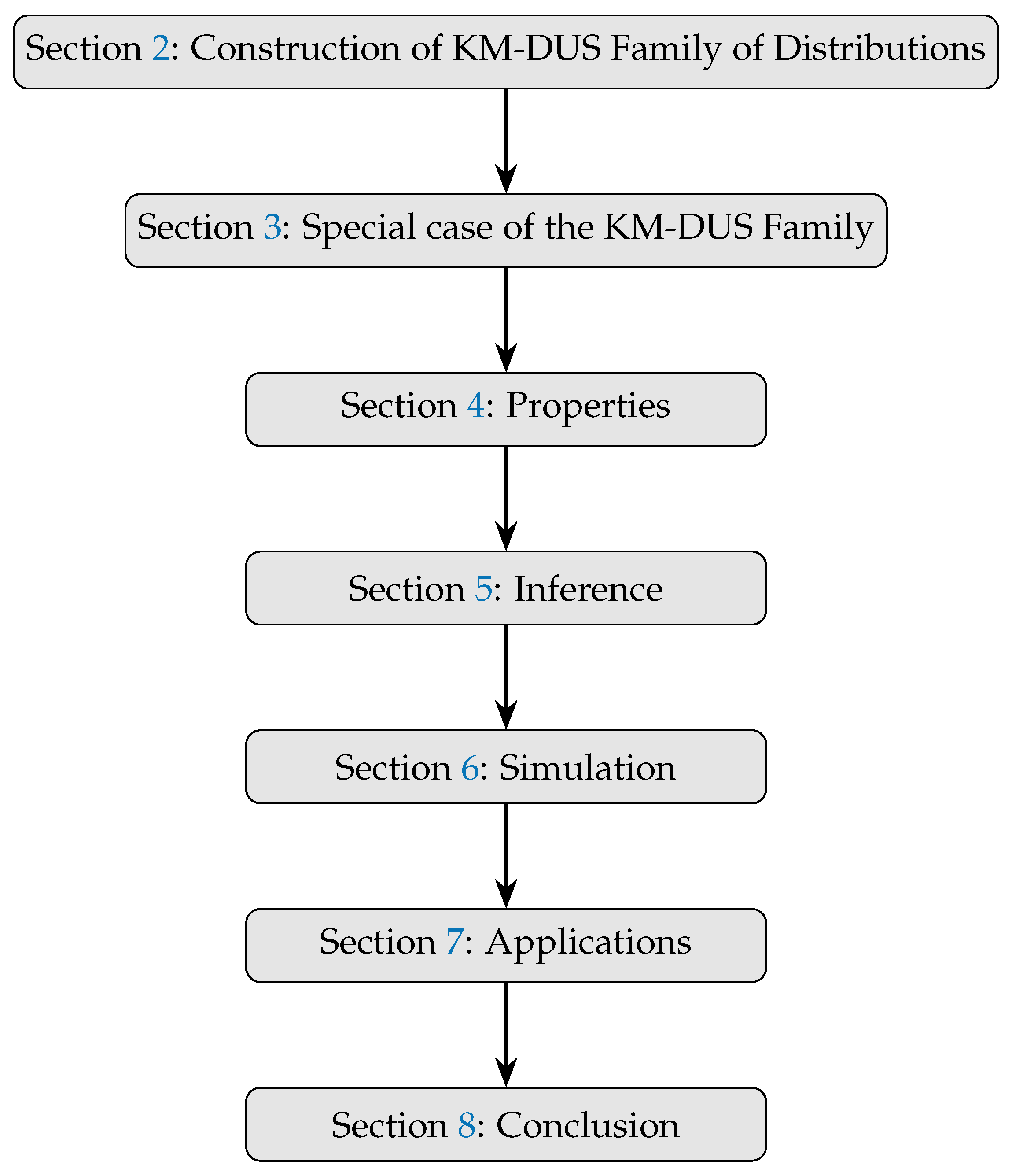
Figure 4.
Mean
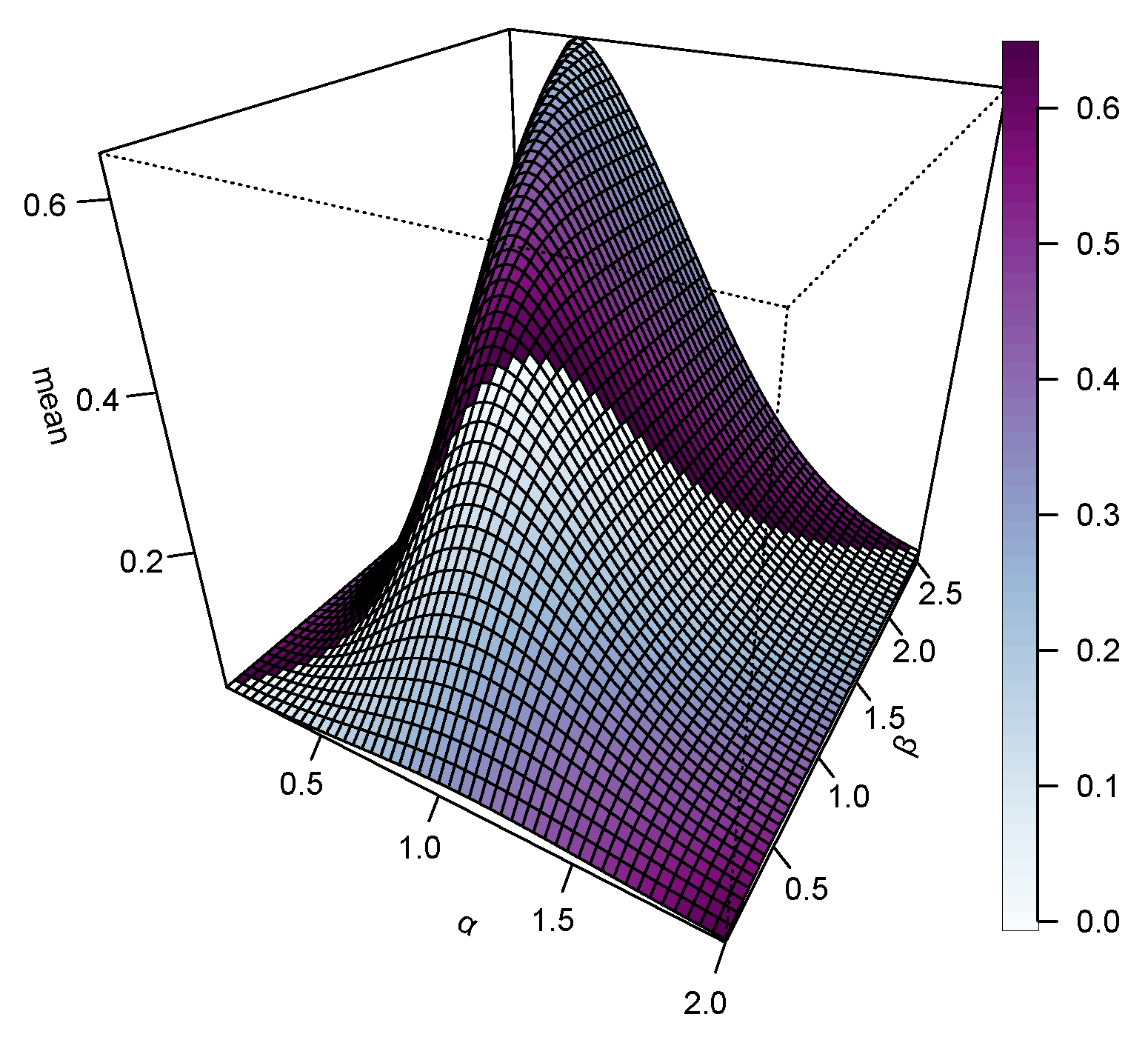
Figure 5.
Variance
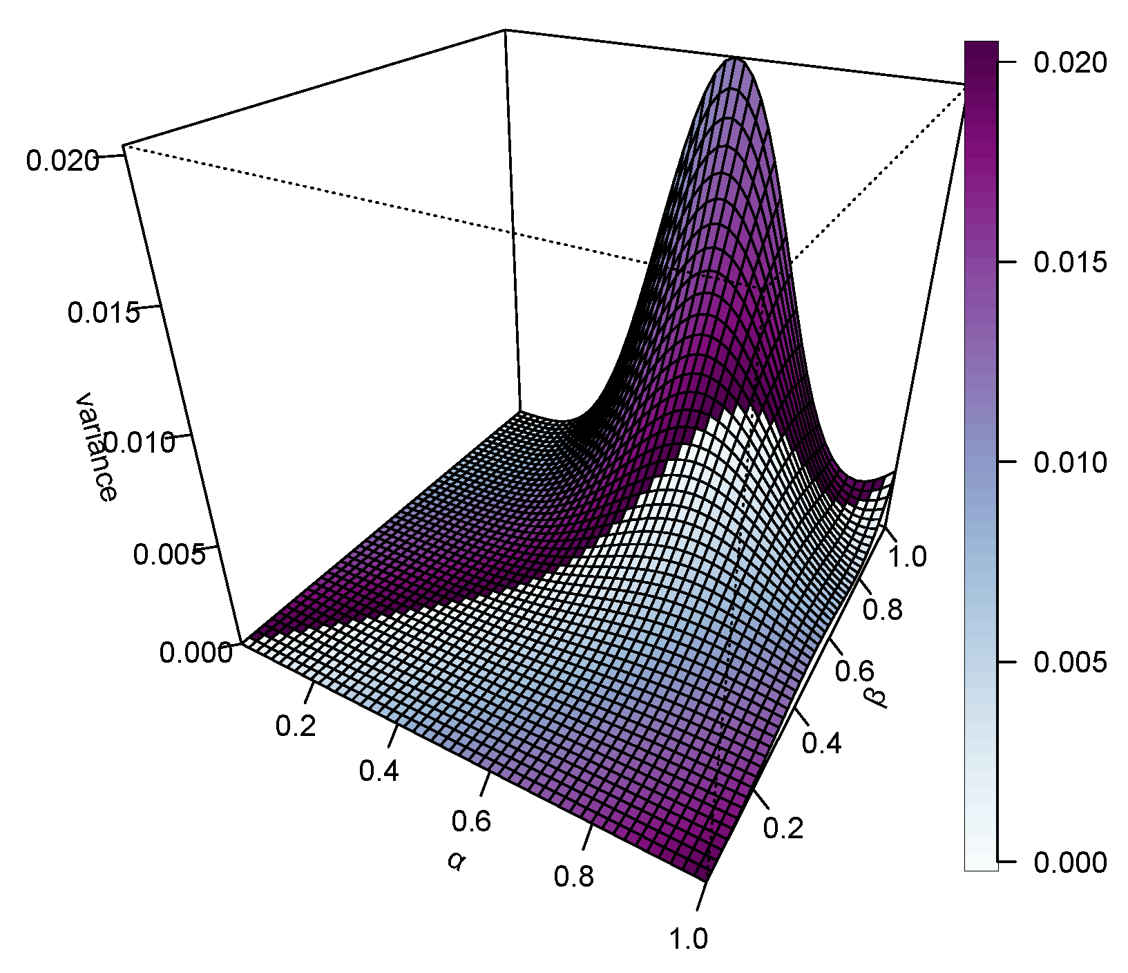
Figure 6.
Skewness
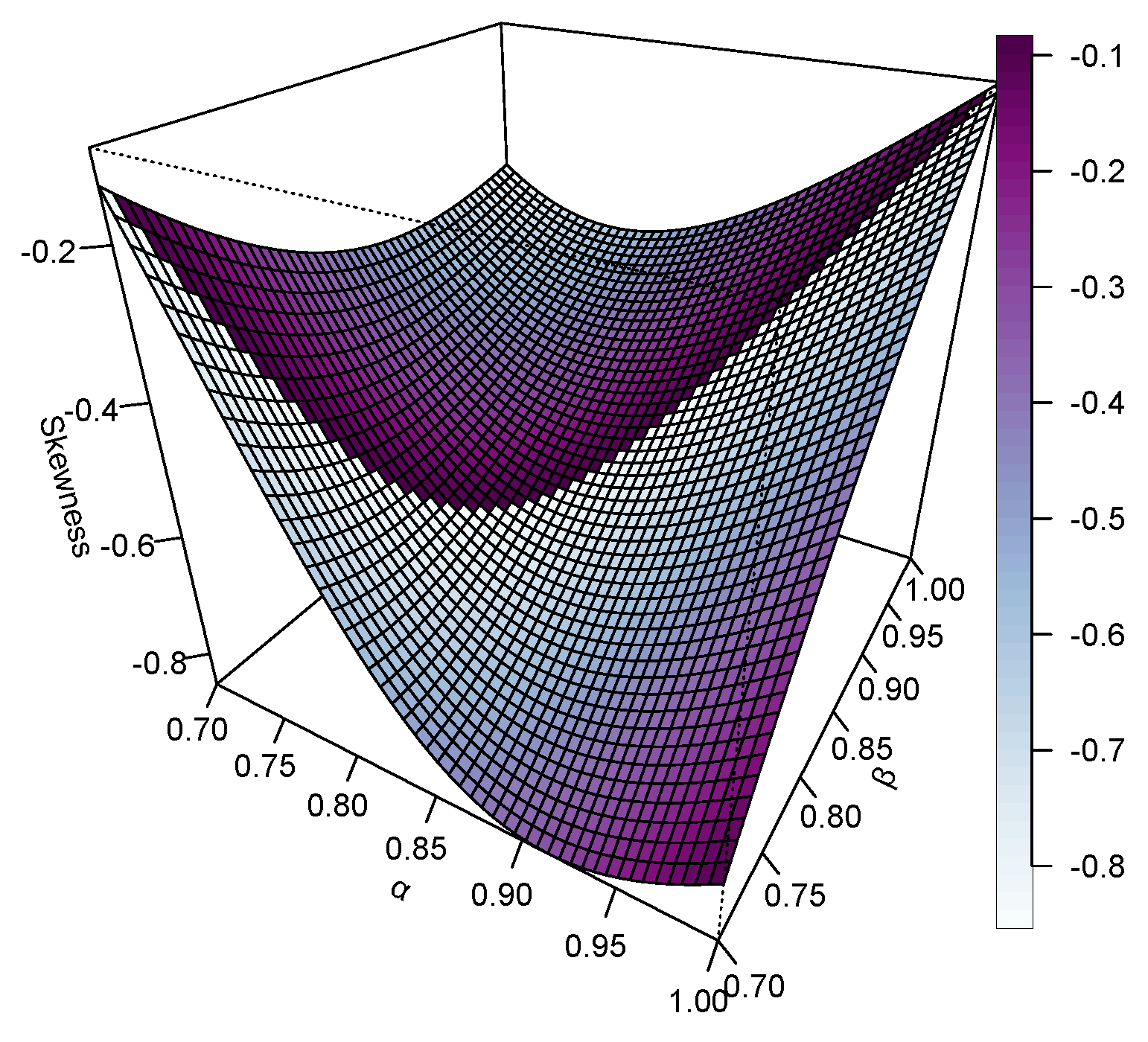
Figure 7.
Kurtosis
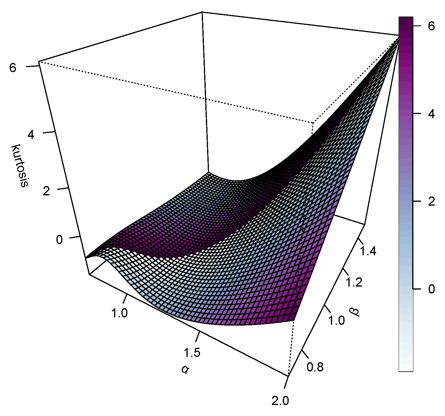
Figure 8.
Box plot for Data-I
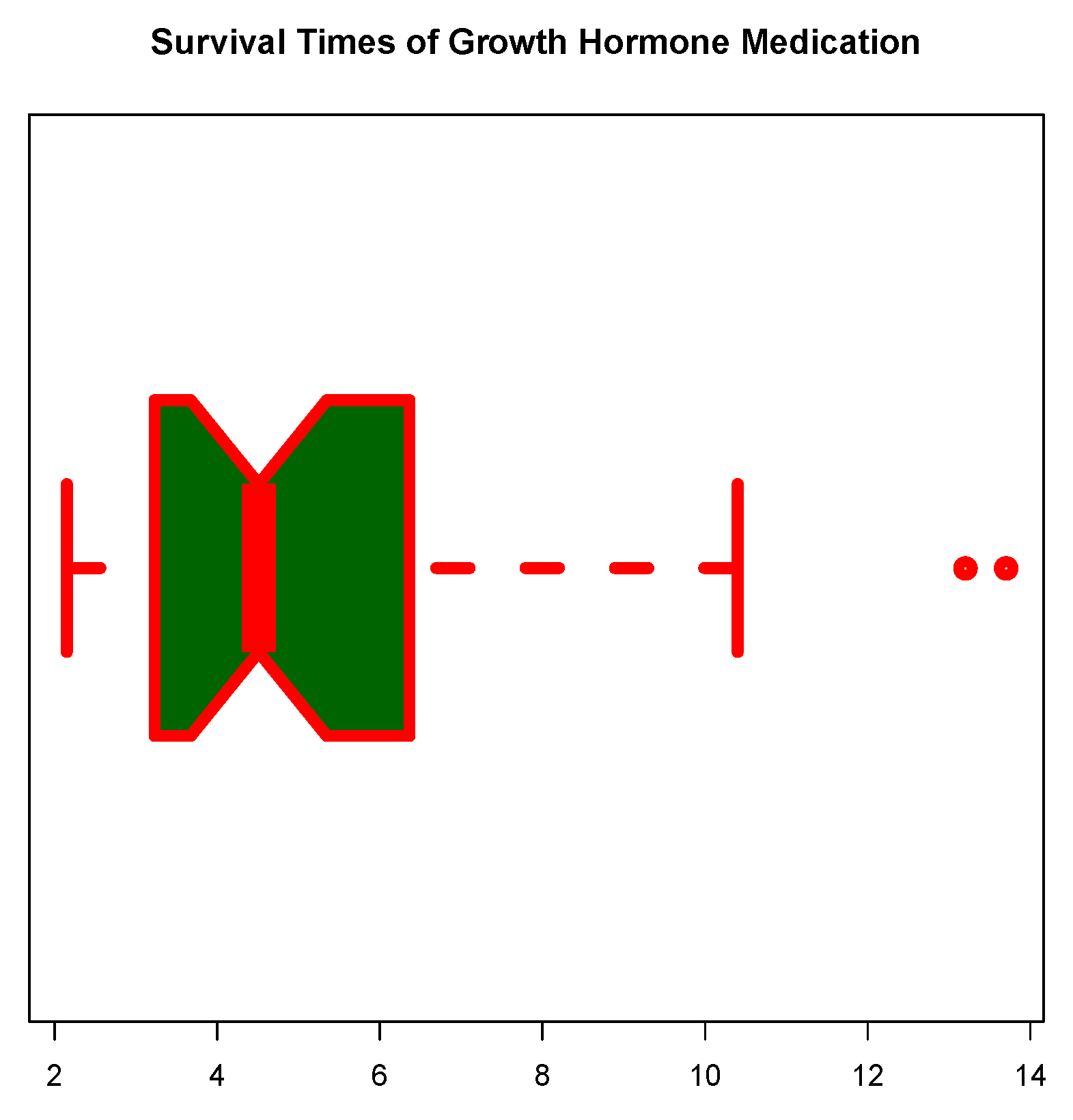
Figure 9.
Box plot for Data-II
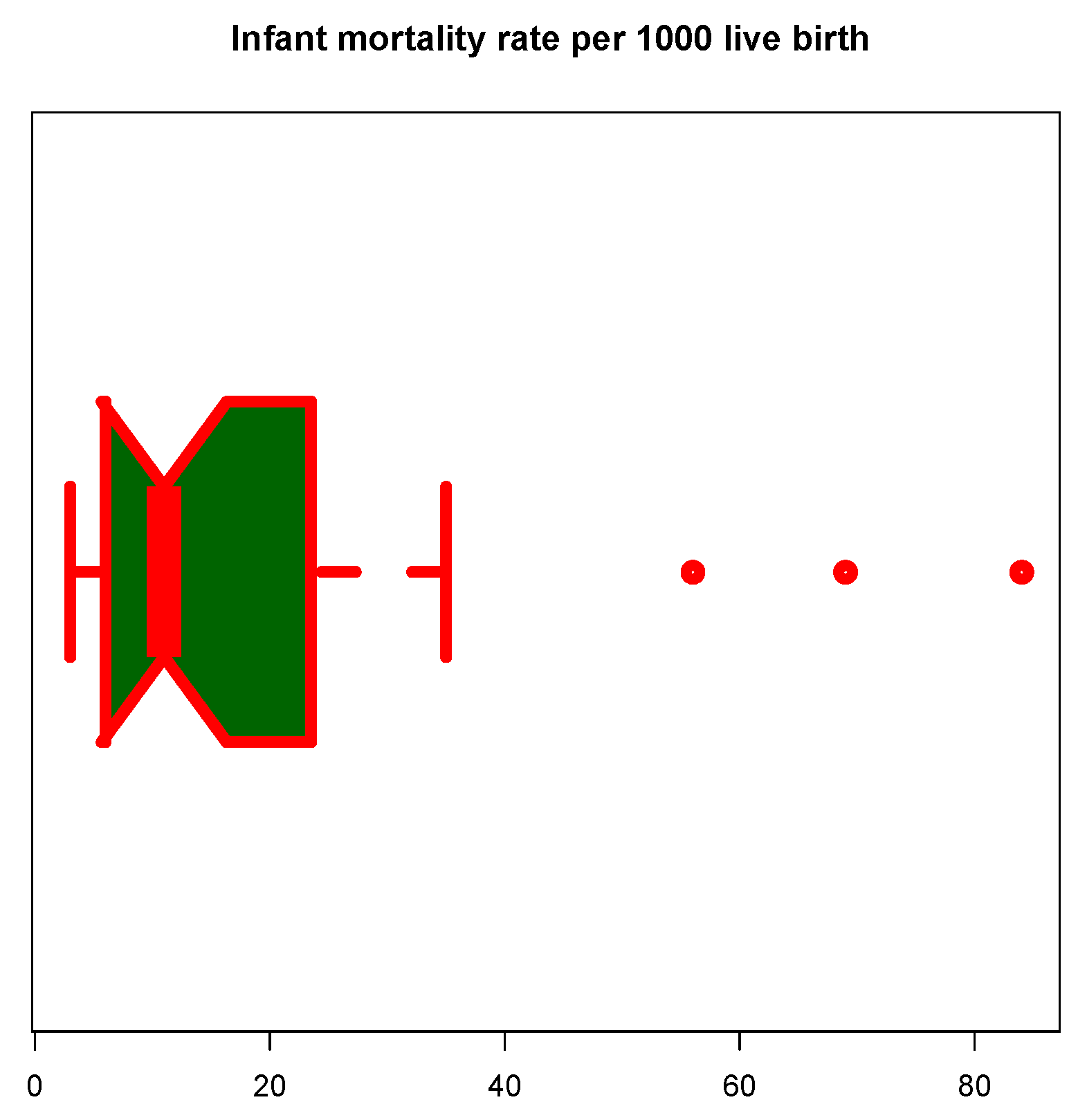
Figure 10.
Density on Histogram for Data-I
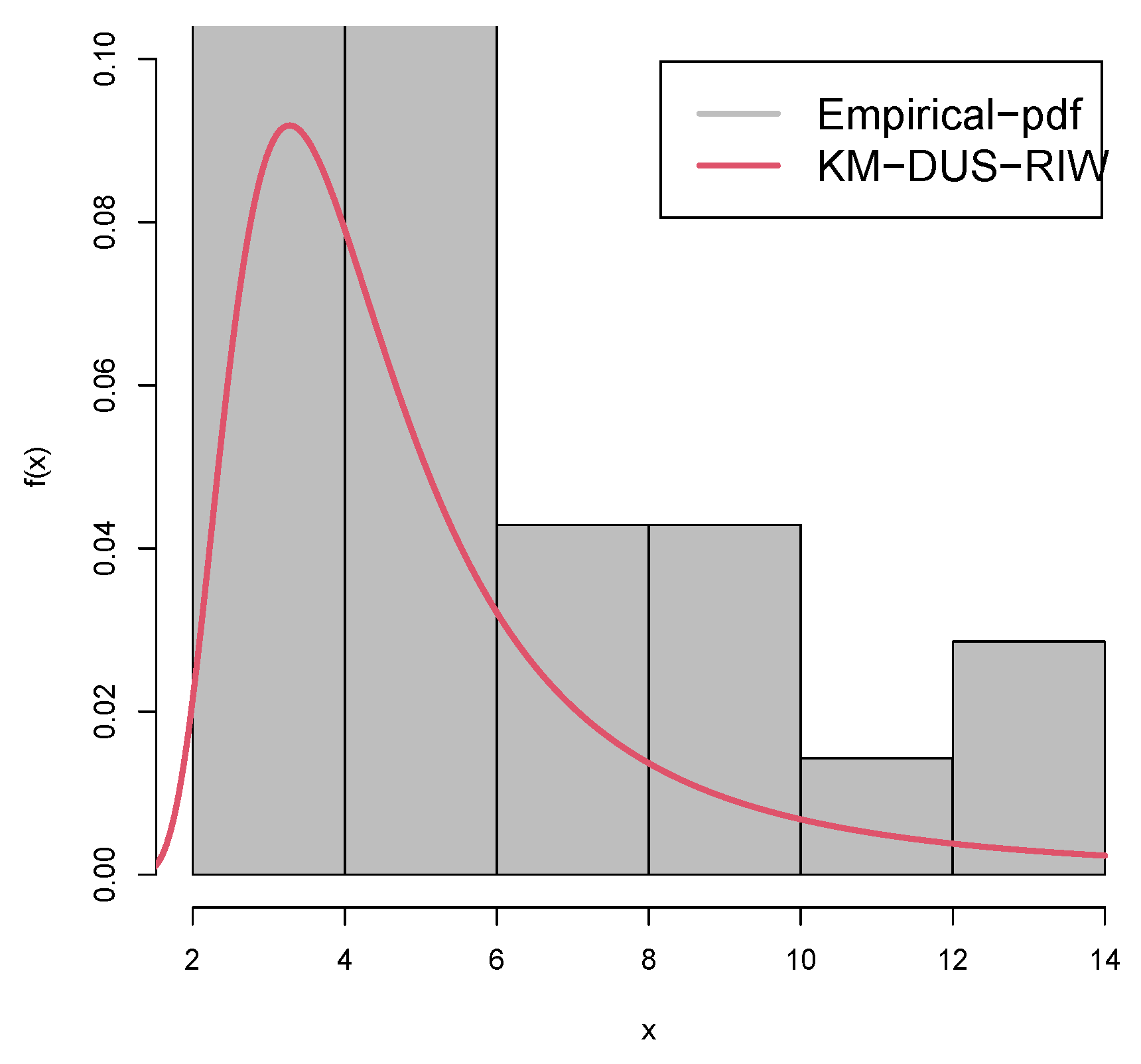
Figure 11.
Density on Histogram for Data-II
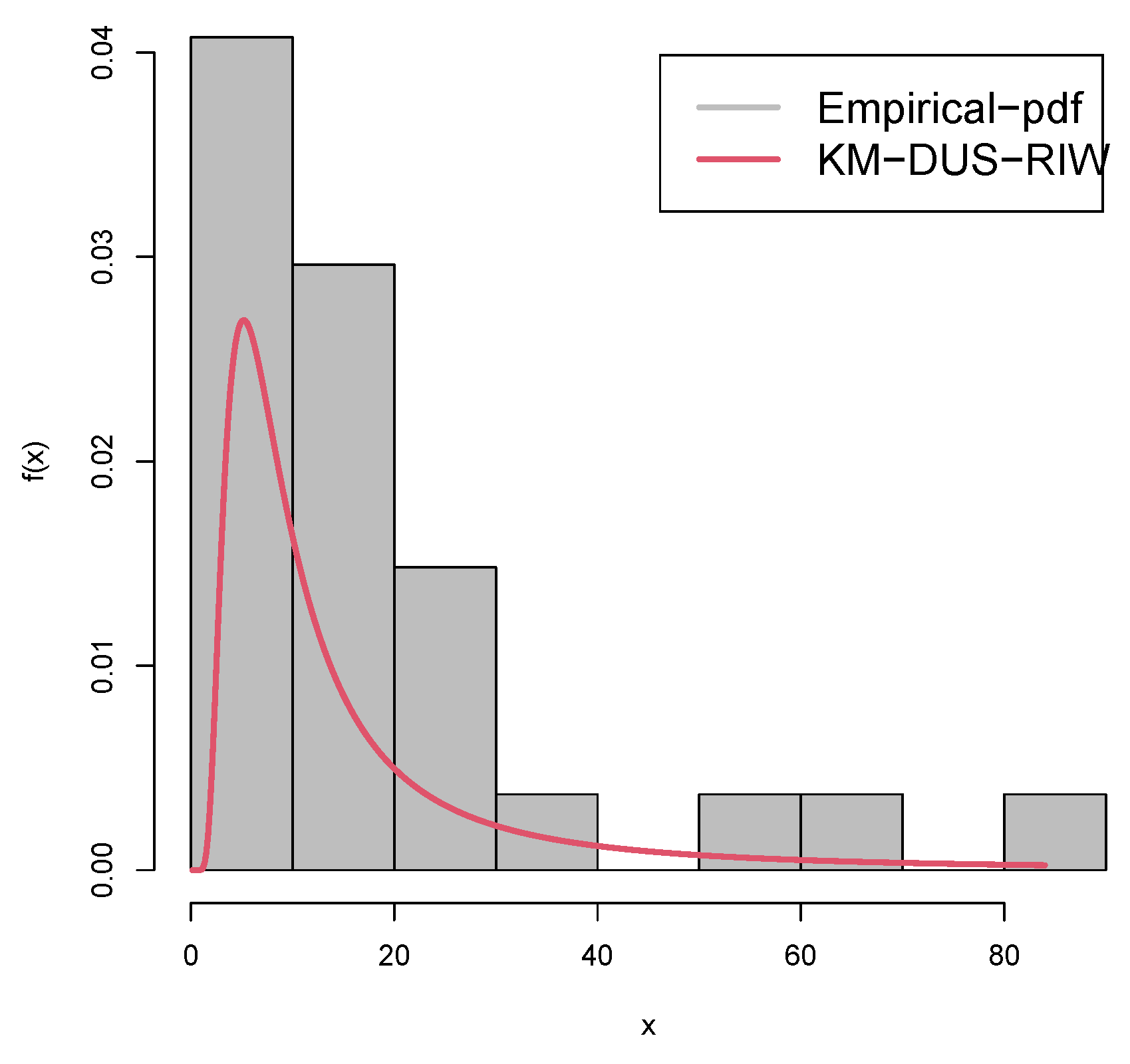
Figure 12.
Contour plot for Data-I
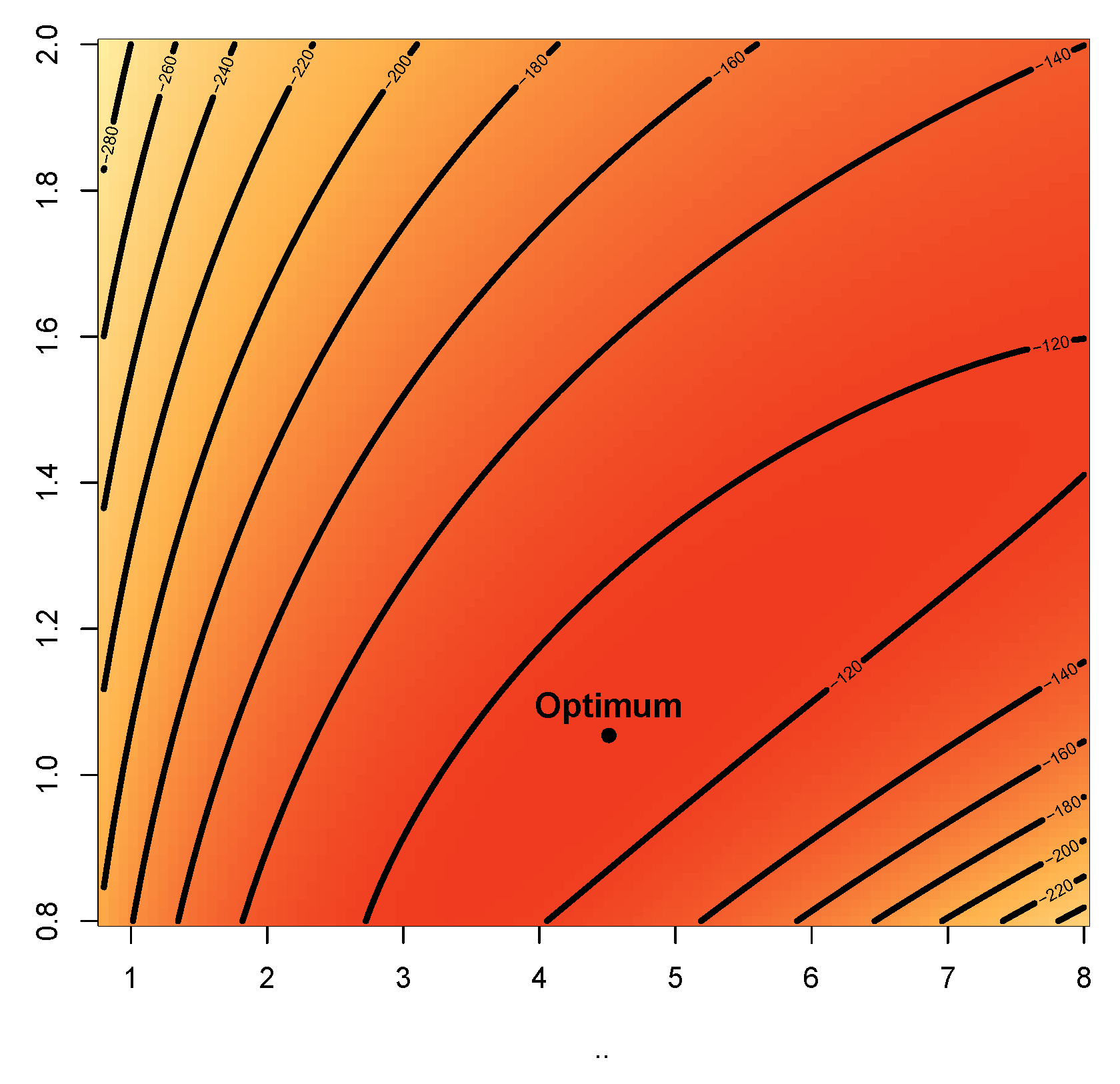
Figure 13.
Contour plot for Data-II
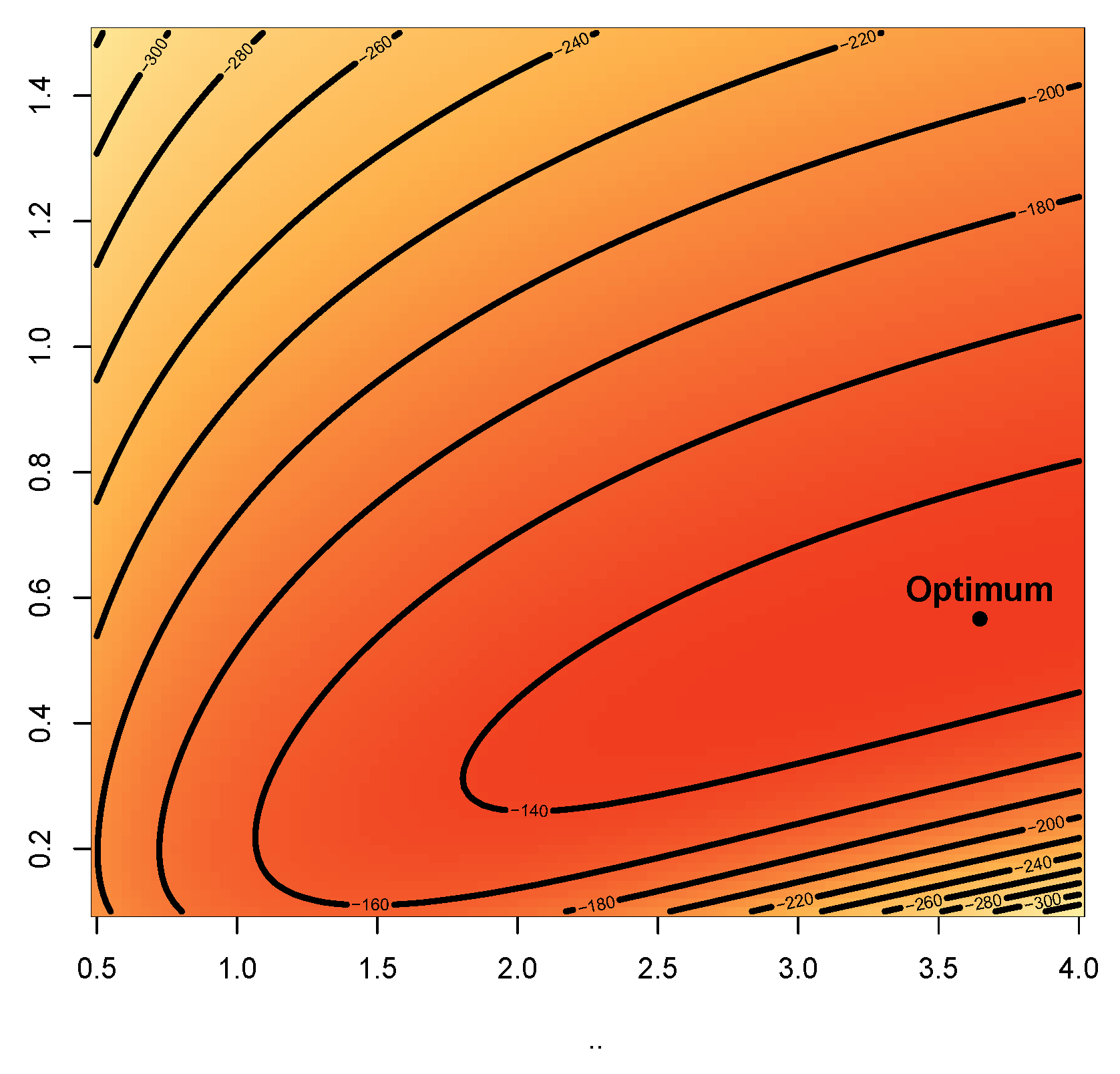
Figure 14.
CDF for Data-I
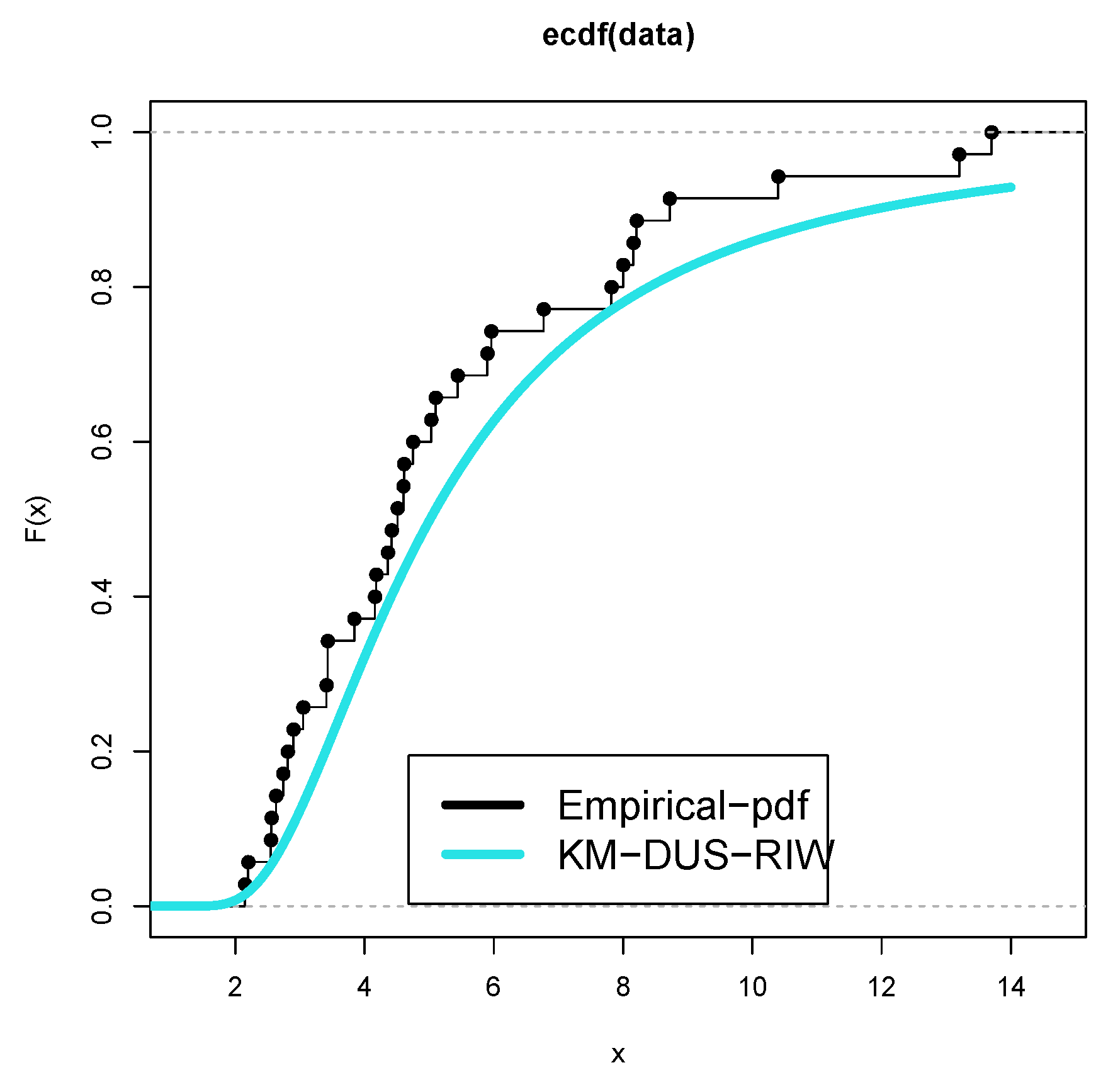
Figure 15.
CDF plot for Data-II
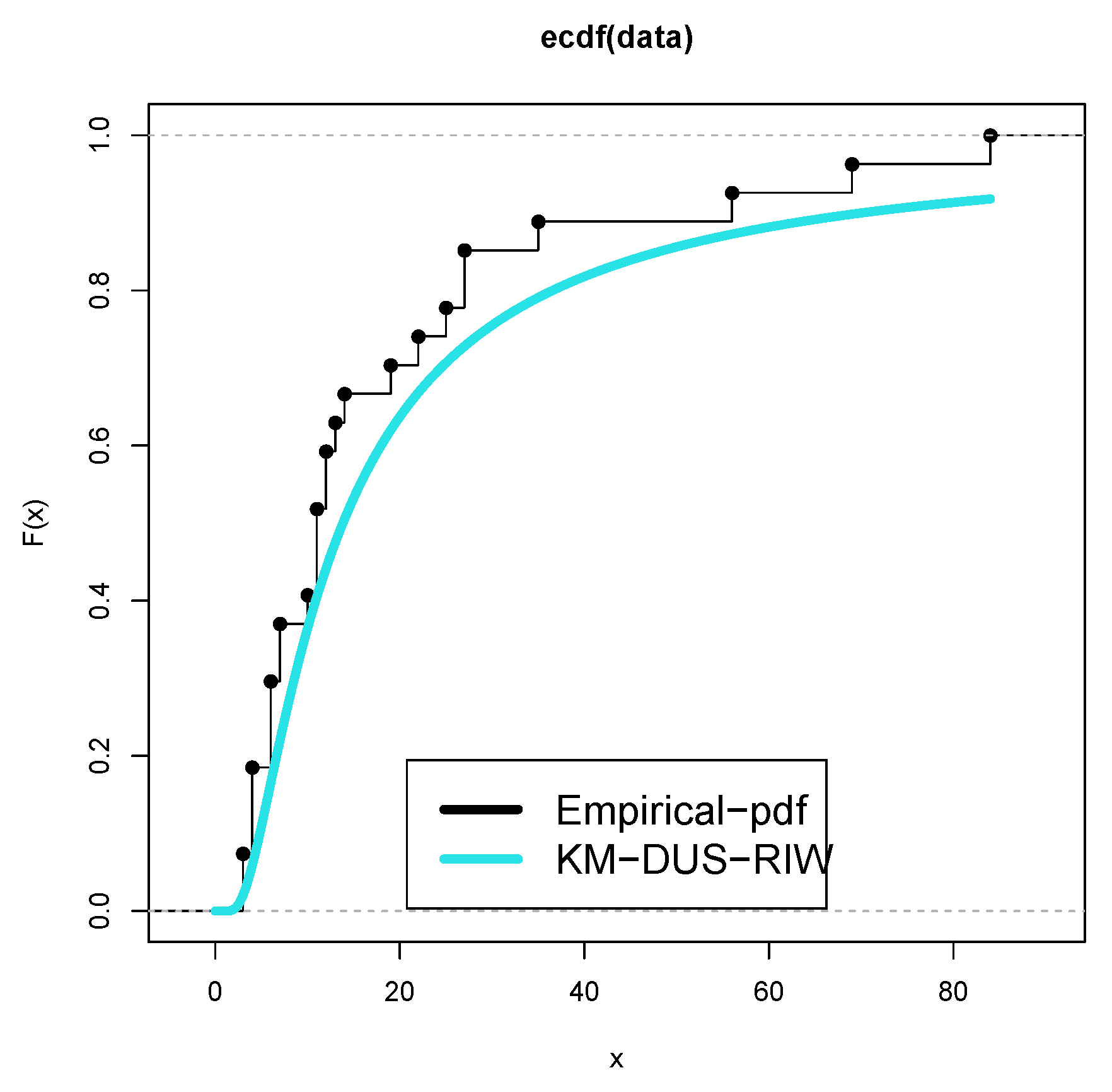
Figure 16.
PP plot for Data-I
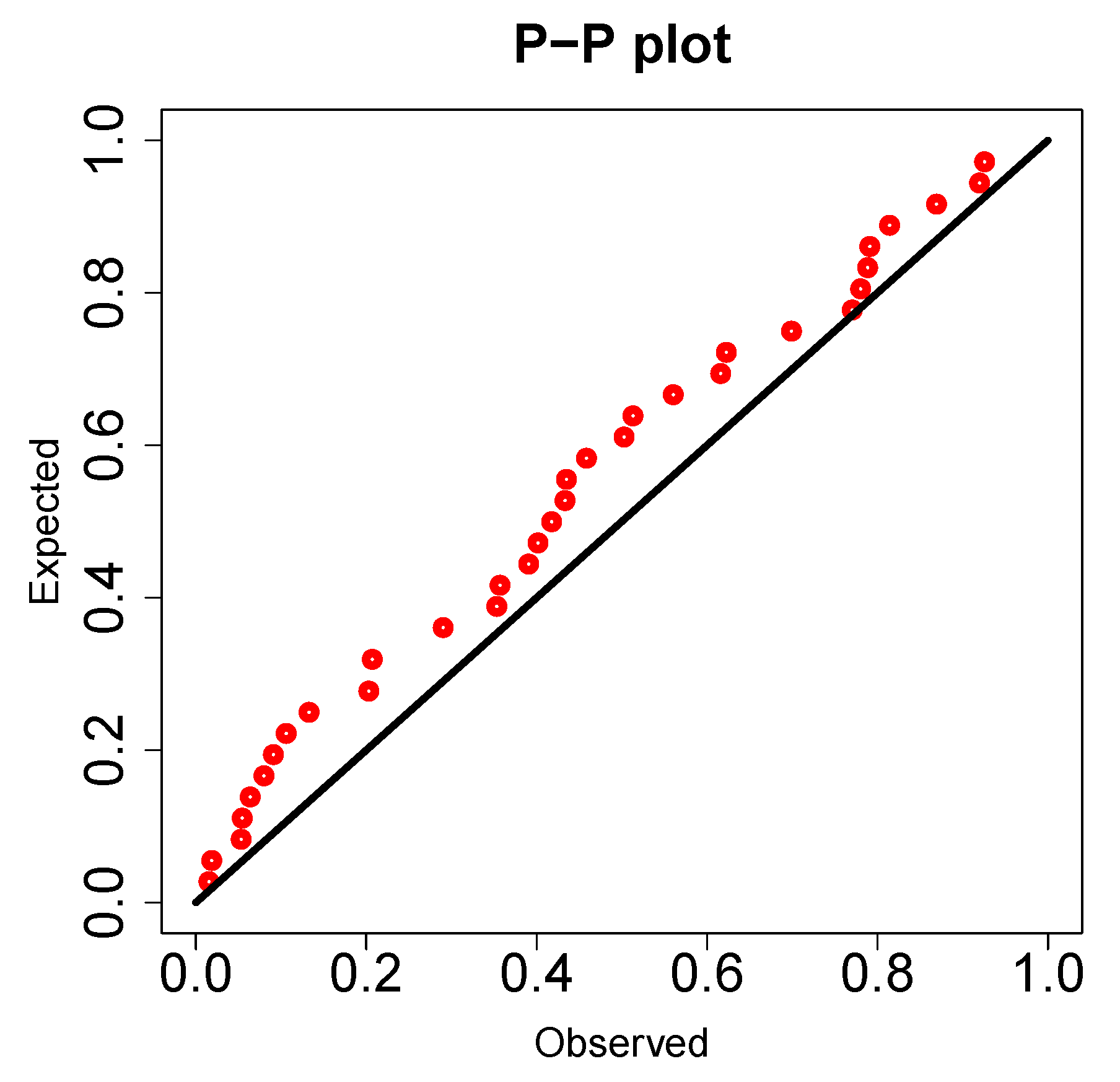
Figure 17.
PP plot for Data-II
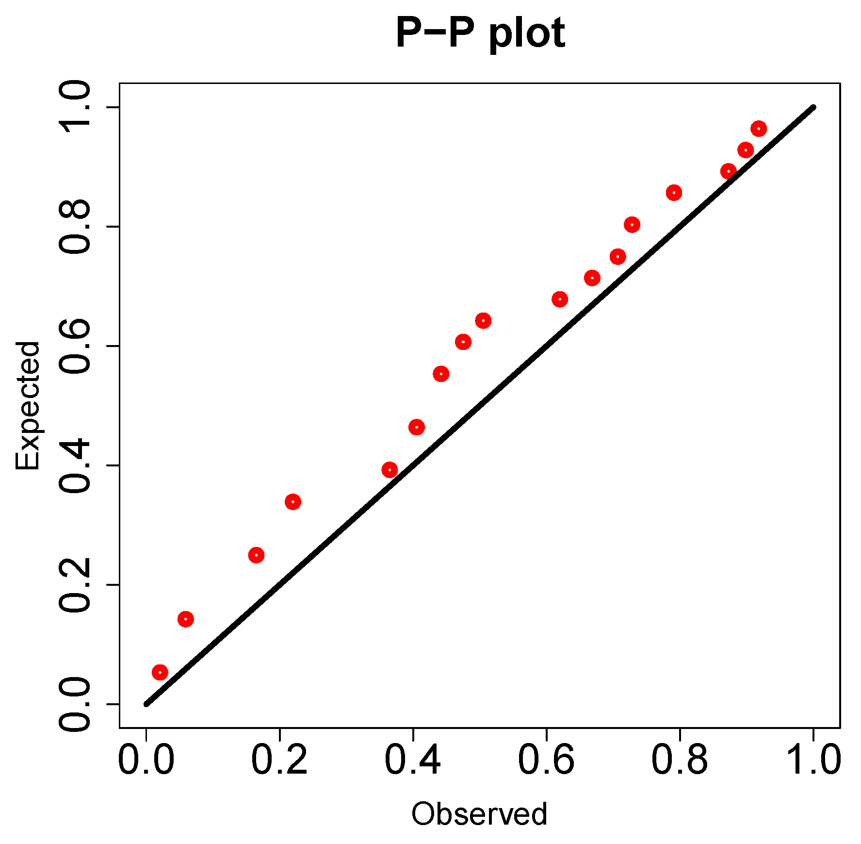
Figure 18.
TTT plot for Data-I
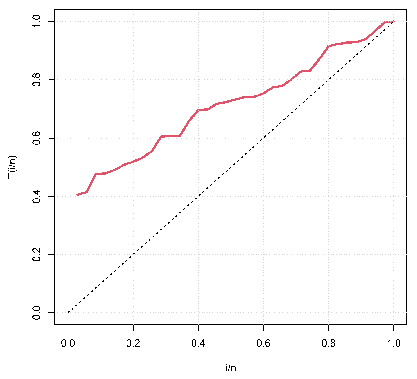
Figure 19.
TTT plot for Data-II
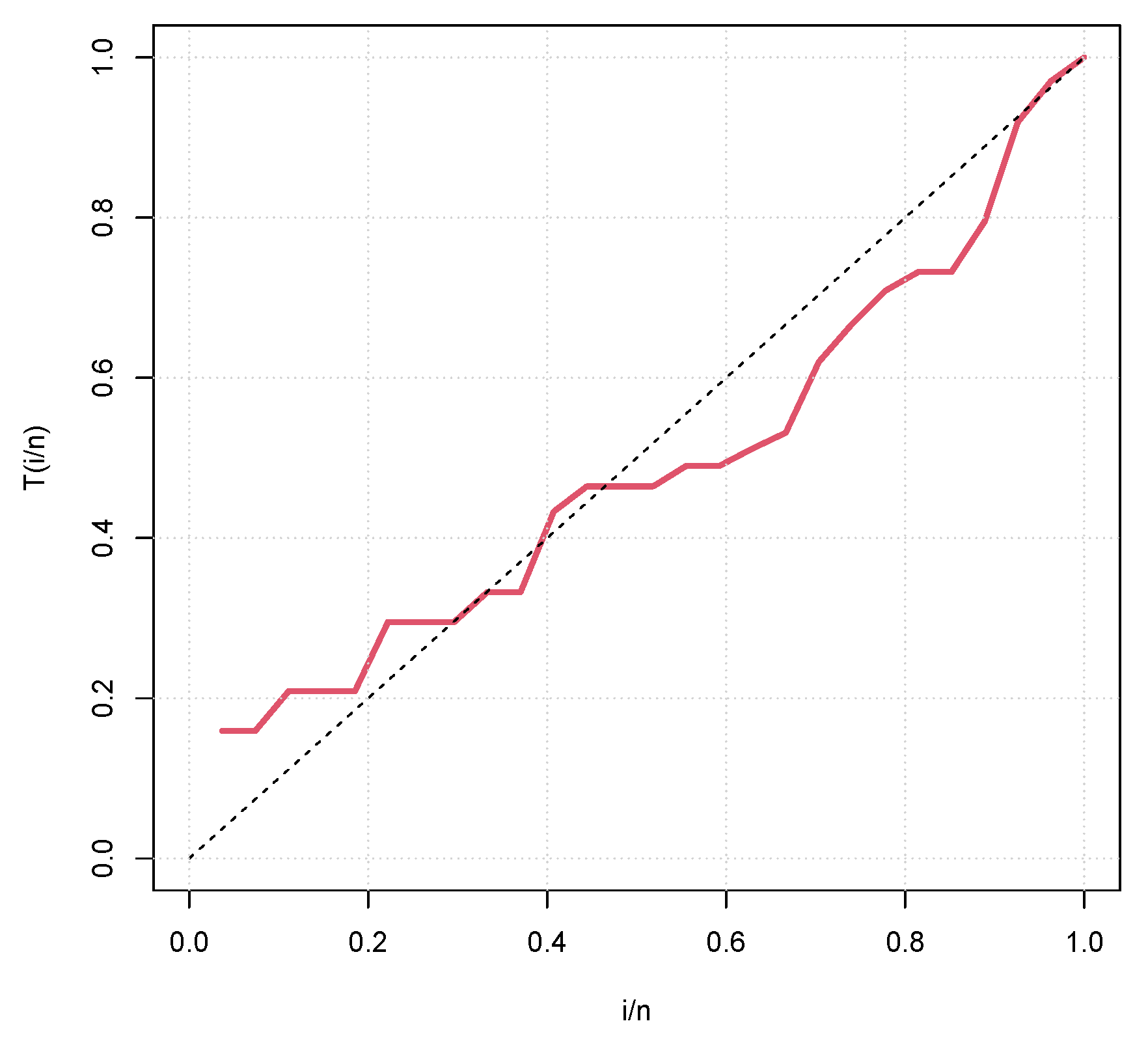

Table 1.
Summary of Literature on Families of Distributions
| Author(s) | Model Developed |
|---|---|
| Alzaatreh et al. [12] | Family of Generalized Gamma Distributions |
| Gupta and Kundu [13] | Exponentiated Exponential Family |
| Chipepa et al. [14] | Generalized Family of Odd-Lindley Distribution |
| Eugene et al. [15] | Beta-Generated Family of Distributions |
| Jones [16] | Extension of Beta-Generated Distributions |
| Ramos et al. [17] | Kumaraswamy-G Poisson Family (Kw-GP) |
| Tahir et al. [18] | New Kumaraswamy Generalized Family of Distributions |
| Afifya et al. [19] | Kumaraswamy Transmuted-G Family |
| Chesneau and Jamal [20] | Sine Kumaraswamy-G Family |
| Arshad et al. [21] | Gamma Kumaraswamy-G Family |
| Ahmed et al. [22] | New Kumaraswamy Kumaraswamy Family of Generalized Distributions |
| Chakraborty et al. [23] | Kumaraswamy Poisson-G Family |
| Jamal et al. [24] | Generalized Inverted Kumaraswamy-G Family |
| Alizadeh et al. [25] | Odd Log-Logistic Poisson-G Family |
| Alzaatreh et al. [8] | Family of Distributions |
| Tahir et al. [26] | Logistic-X (LX) Family |
| Elbatal et al. [27] | Odd-Perks-G Family |
| Cordeiro and De Castro [28] | Kumaraswamy-G (K-G) Family |
| Anzagra et al. [29] | Chen-G Class of Distributions |
| Rezaei et al. [30] | Topp-Leone Generated Family |
| Kumar et al. [6] | Dinesh-Umesh-Sanjay (DUS) Family |
| Cordeiro et al. [31] | Type I Half-Logistic Family |
Table 2.
Further Selected Distribution Families from Literature
| Family | Base Model/Transformation | Reference |
|---|---|---|
| Alpha-log-power transformed-G (ALPT-G) | General transformation without a specific base distribution; applied to Burr-XII | Musekwa et al. [32] |
| Alpha-power exponential (APE) | Alpha-power transformation of the exponential distribution | Mahdavi and Kundu [33] |
| Alpha-power transformed-G (APTG) | General transformation adding shape parameter to a baseline G | Mahdavi and Kundu [33] |
| Arctan-X | Trigonometric-based family using the arctangent function | Alkhairy et al. [34] |
| Burr-Hatke-G | Burr-Hatke differential equation with regression model | Yousof et al. [35] |
| EHL-PGW-G (Exponentiated Half Logistic Power Generalized-G) | Generalization of Power Generalized Weibull-G using exponentiated half-logistic | Oluyede et al. [36] |
| Extended cosine-G | Weighted cosine transformation of the SG family | Muhammad et al. [37] |
| Extended Odd Frechet | (T-X)-based family using extended Frechet | Yousof et al. [38] |
| Gamma-X | Weibull as X, forming Generalized Gamma distribution | Loving [39] |
| Generalized odd log-logistic-G | Uses regression model for survival analysis | Cordeiro et al. [40] |
| Gudermanian generated | Based on the Gudermanian function with heteroscedastic regression model | Altun et al. [41] |
| NFGF (New Flexible Generalized Family) | Independent of parent model; applied to Kumaraswamy (NFKw) | Tahir et al. [42] |
| Odd Lindley-G | Uses and | Gomes-Silva et al. [43] |
| Odd log-logistic Topp-Leone G | Heteroscedastic regression model for survival data with cured fraction | Alizadeh et al. [25] |
| Odd power Cauchy-G | Regression model-based, transformation involving power of odd function | Alizadeh et al. [25] |
| Power Lindley-G | Power Lindley distribution as generator | Hassan and Nassr [44] |
| Rank Transmutation Maps (RTM) | Transformation: | Shaw and Buckley [45] |
| TI-HT (Type-I Heavy Tailed) | Transformed version of any to create heavy-tailed behavior | Zhao [46] |
| Topp-Leone-G | Uses Topp-Leone generator | Al-Shomrani et al. [47] |
| Transmuted-G (Quadratic) | Shaw and Buckley [45] | |
| T-X family | Transformation: , where T and X are independent | Alzaatreh et al. [8] |
| Type I half-logistic exponentiated-G | Exponentiated-G with Type I half-logistic generator | Bello et al. [48] |
| Type II log-logistic | Generalization of log-logistic using transformation | Soliman et al. [49] |
| Weighted cosine-G | Trigonometric cosine-based generator | Odhah et al. [50] |
Table 3.
Summary of Basic Statistics
| Parameters | n | Sk | Ku | CV | |||
| 25 | 0.03318 | 0.00071 | 0.02662 | 2.13429 | 4.98791 | 0.80236 | |
| 50 | 0.07318 | 0.03151 | 0.17750 | 4.14230 | 17.48965 | 2.42543 | |
| 100 | 0.03905 | 0.00107 | 0.03269 | 1.60763 | 2.25682 | 0.83710 | |
| 200 | 0.04096 | 0.00376 | 0.06133 | 6.38540 | 56.10753 | 1.49720 | |
| 500 | 0.04268 | 0.00524 | 0.07236 | 7.71392 | 81.25716 | 1.69566 | |
| 1000 | 0.04920 | 0.02126 | 0.14580 | 13.10721 | 202.11051 | 2.96376 | |
| 25 | 0.71474 | 0.32889 | 0.57349 | 2.13434 | 4.98765 | 0.80237 | |
| 50 | 1.57668 | 14.62379 | 3.82411 | 4.14229 | 17.48947 | 2.42541 | |
| 100 | 0.84124 | 0.49593 | 0.70422 | 1.60766 | 2.25680 | 0.83712 | |
| 200 | 0.88251 | 1.74589 | 1.32132 | 6.38551 | 56.10907 | 1.49723 | |
| 500 | 0.91935 | 2.43054 | 1.55902 | 7.71400 | 81.25905 | 1.69578 | |
| 1000 | 1.05986 | 9.86757 | 3.14127 | 13.10724 | 202.11099 | 2.96385 | |
| 25 | 0.12246 | 0.00290 | 0.05388 | 1.39762 | 2.12205 | 0.43995 | |
| 50 | 0.15985 | 0.03220 | 0.17944 | 3.37554 | 11.54481 | 1.12251 | |
| 100 | 0.13313 | 0.00418 | 0.06464 | 1.06624 | 0.47825 | 0.48555 | |
| 200 | 0.13057 | 0.00764 | 0.08740 | 3.20392 | 16.80312 | 0.66937 | |
| 500 | 0.13308 | 0.00857 | 0.09260 | 4.01334 | 25.02845 | 0.69577 | |
| 1000 | 0.13629 | 0.01580 | 0.12570 | 7.00607 | 72.74627 | 0.92233 | |
| 25 | 0.79741 | 0.08216 | 0.28664 | 1.20704 | 1.54260 | 0.35946 | |
| 50 | 0.96004 | 0.66838 | 0.81754 | 3.12661 | 9.94955 | 0.85157 | |
| 100 | 0.85196 | 0.11656 | 0.34141 | 0.93250 | 0.14918 | 0.40073 | |
| 200 | 0.83190 | 0.19140 | 0.43750 | 2.59530 | 11.27701 | 0.52590 | |
| 500 | 0.84548 | 0.20493 | 0.45269 | 3.29479 | 17.21825 | 0.53542 | |
| 1000 | 0.85595 | 0.32753 | 0.57230 | 5.50241 | 48.03277 | 0.66861 | |
| 25 | 0.21942 | 0.00445 | 0.06672 | 1.07014 | 1.17137 | 0.30409 | |
| 50 | 0.25210 | 0.02938 | 0.17141 | 2.93216 | 8.79434 | 0.67994 | |
| 100 | 0.23173 | 0.00625 | 0.07903 | 0.83718 | -0.05746 | 0.34105 | |
| 200 | 0.22608 | 0.00962 | 0.09809 | 2.21727 | 8.26887 | 0.43385 | |
| 500 | 0.22934 | 0.00998 | 0.09990 | 2.84354 | 12.94875 | 0.43559 | |
| 1000 | 0.23090 | 0.01466 | 0.12106 | 4.55886 | 34.39667 | 0.52431 | |
| 25 | 0.83493 | 0.04845 | 0.22011 | 0.96800 | 0.91908 | 0.26362 | |
| 50 | 0.93126 | 0.27535 | 0.52474 | 2.77772 | 7.92751 | 0.56347 | |
| 100 | 0.87451 | 0.06736 | 0.25954 | 0.76604 | -0.19621 | 0.29679 | |
| 200 | 0.85364 | 0.09956 | 0.31553 | 1.96308 | 6.44925 | 0.36964 | |
| 500 | 0.86470 | 0.10096 | 0.31775 | 2.53746 | 10.35448 | 0.36747 | |
| 1000 | 0.86798 | 0.14044 | 0.37475 | 3.93510 | 26.30485 | 0.43175 |
Table 4.
Case I Simulation Outcome
| Parameter | Metric | MLE | MPS | LS | WLS | CVM | AD | RTAD | PERC | BE | BE | BE | BE | BE |
| Bias () | 0.20718 | 0.05923 | 0.01453 | 0.02188 | 0.10314 | 0.03217 | 0.09998 | 0.07179 | 0.33448 | 0.34675 | 0.32249 | 0.32882 | 0.31756 | |
| Bias () | 0.16240 | 0.02816 | 0.01453 | 0.01922 | 0.04133 | 0.01955 | 0.03886 | 0.06404 | 0.40969 | 0.41475 | 0.40467 | 0.40738 | 0.40276 | |
| Bias () | 0.14445 | 0.02196 | 0.00267 | 0.00676 | 0.01558 | 0.00571 | 0.01480 | 0.06225 | 0.43351 | 0.43619 | 0.43085 | 0.43230 | 0.42986 | |
| Bias () | 0.14298 | 0.01673 | 0.00247 | 0.00619 | 0.01209 | 0.00541 | 0.00986 | 0.06145 | 0.43769 | 0.43971 | 0.43567 | 0.43677 | 0.43492 | |
| RMSE () | 0.09898 | 0.04548 | 0.08316 | 0.07220 | 0.12084 | 0.06204 | 0.15953 | 0.12287 | 0.16122 | 0.17158 | 0.15154 | 0.15691 | 0.14858 | |
| RMSE () | 0.04163 | 0.01477 | 0.02664 | 0.02153 | 0.03047 | 0.01961 | 0.03509 | 0.05392 | 0.18280 | 0.18722 | 0.17847 | 0.18083 | 0.17694 | |
| RMSE () | 0.02790 | 0.00739 | 0.01129 | 0.00920 | 0.01199 | 0.00877 | 0.01427 | 0.03524 | 0.19579 | 0.19819 | 0.19342 | 0.19472 | 0.19257 | |
| RMSE () | 0.02563 | 0.00550 | 0.00756 | 0.00637 | 0.00792 | 0.00618 | 0.00997 | 0.03240 | 0.19780 | 0.19962 | 0.19599 | 0.19698 | 0.19534 | |
| Bias () | 0.15922 | 0.17169 | 0.01220 | 0.01208 | 0.16638 | 0.03876 | 0.11771 | 0.22456 | 0.08235 | 0.12281 | 0.04341 | 0.06862 | 0.04119 | |
| Bias () | 0.23565 | 0.07720 | 0.01829 | 0.03283 | 0.07526 | 0.03417 | 0.06029 | 0.14900 | 0.25180 | 0.27016 | 0.23370 | 0.24576 | 0.23368 | |
| Bias () | 0.27527 | 0.06276 | 0.00496 | 0.00626 | 0.02296 | 0.00359 | 0.01614 | 0.13733 | 0.30242 | 0.31234 | 0.29259 | 0.29920 | 0.29275 | |
| Bias () | 0.27369 | 0.04499 | 0.00342 | 0.01215 | 0.02437 | 0.00997 | 0.01533 | 0.12640 | 0.31270 | 0.32023 | 0.30522 | 0.31026 | 0.30536 | |
| RMSE () | 0.20038 | 0.20480 | 0.29014 | 0.25366 | 0.37052 | 0.22054 | 0.37772 | 0.47321 | 0.18607 | 0.20510 | 0.17225 | 0.18246 | 0.17675 | |
| RMSE () | 0.11374 | 0.07216 | 0.10766 | 0.08928 | 0.11854 | 0.08422 | 0.12020 | 0.22073 | 0.11909 | 0.13014 | 0.10895 | 0.11585 | 0.10960 | |
| RMSE () | 0.10057 | 0.03304 | 0.04505 | 0.03627 | 0.04672 | 0.03500 | 0.04880 | 0.13123 | 0.11979 | 0.12627 | 0.11356 | 0.11779 | 0.11385 | |
| RMSE () | 0.09498 | 0.02592 | 0.03525 | 0.02933 | 0.03649 | 0.02860 | 0.03867 | 0.12034 | 0.11913 | 0.12412 | 0.11429 | 0.11757 | 0.11449 |
Table 5.
Case II Simulation Outcome
| Parameter | Metric | ML | MPS | LS | WLS | CvM | AD | RTAD | PERC | BE | BE | BE | BE | BE |
| Bias () | 0.18828 | 0.03997 | 0.00264 | 0.00520 | 0.05434 | 0.01528 | 0.05259 | 0.05157 | 0.27685 | 0.28406 | 0.26972 | 0.27289 | 0.26497 | |
| Bias () | 0.15793 | 0.02063 | 0.00404 | 0.00884 | 0.02178 | 0.00867 | 0.02081 | 0.04586 | 0.32529 | 0.32805 | 0.32254 | 0.32379 | 0.32078 | |
| Bias () | 0.15029 | 0.01229 | 0.00175 | 0.00510 | 0.01040 | 0.00486 | 0.01080 | 0.03900 | 0.34022 | 0.34165 | 0.33880 | 0.33945 | 0.33790 | |
| Bias () | 0.14829 | 0.00992 | 0.00250 | 0.00465 | 0.00899 | 0.00418 | 0.00827 | 0.03306 | 0.34255 | 0.34362 | 0.34147 | 0.34197 | 0.34080 | |
| RMSE () | 0.07028 | 0.02748 | 0.04313 | 0.03785 | 0.05817 | 0.03462 | 0.07220 | 0.05056 | 0.10452 | 0.10926 | 0.09998 | 0.10211 | 0.09743 | |
| RMSE () | 0.03412 | 0.00873 | 0.01367 | 0.01157 | 0.01521 | 0.01068 | 0.01934 | 0.02561 | 0.11447 | 0.11637 | 0.11261 | 0.11347 | 0.11147 | |
| RMSE () | 0.02685 | 0.00424 | 0.00654 | 0.00534 | 0.00689 | 0.00513 | 0.00832 | 0.01413 | 0.12025 | 0.12125 | 0.11926 | 0.11972 | 0.11865 | |
| RMSE () | 0.02504 | 0.00307 | 0.00447 | 0.00373 | 0.00467 | 0.00358 | 0.00557 | 0.01163 | 0.12087 | 0.12162 | 0.12012 | 0.12046 | 0.11966 | |
| Bias () | 0.16280 | 0.17678 | 0.02042 | 0.01642 | 0.18842 | 0.05850 | 0.13179 | 0.23793 | 0.07480 | 0.13295 | 0.01931 | 0.05805 | 0.02462 | |
| Bias () | 0.29162 | 0.10673 | 0.00015 | 0.02181 | 0.06704 | 0.02065 | 0.04489 | 0.19113 | 0.29098 | 0.31700 | 0.26542 | 0.28375 | 0.26926 | |
| Bias () | 0.30942 | 0.05674 | 0.00381 | 0.02001 | 0.03682 | 0.01837 | 0.03170 | 0.13494 | 0.35522 | 0.36916 | 0.34141 | 0.35138 | 0.34370 | |
| Bias () | 0.32762 | 0.05734 | 0.00266 | 0.00736 | 0.02209 | 0.00498 | 0.01436 | 0.12677 | 0.36747 | 0.37807 | 0.35694 | 0.36456 | 0.35872 | |
| RMSE () | 0.32410 | 0.32583 | 0.45707 | 0.40350 | 0.57011 | 0.36884 | 0.54112 | 0.59847 | 0.24641 | 0.27682 | 0.22651 | 0.24193 | 0.23517 | |
| RMSE () | 0.16183 | 0.09792 | 0.13894 | 0.11699 | 0.15069 | 0.10810 | 0.15884 | 0.28337 | 0.16111 | 0.17940 | 0.14462 | 0.15660 | 0.14793 | |
| RMSE () | 0.13288 | 0.04744 | 0.06633 | 0.05510 | 0.06934 | 0.05280 | 0.07605 | 0.16510 | 0.16563 | 0.17639 | 0.15539 | 0.16283 | 0.15732 | |
| RMSE () | 0.13367 | 0.03437 | 0.04899 | 0.03980 | 0.05039 | 0.03845 | 0.05368 | 0.11980 | 0.16470 | 0.17297 | 0.15672 | 0.16251 | 0.15820 |
Table 6.
Case III Simulation Outcome
| Parameter | Metric | ML | MPS | LS | WLS | CvM | AD | RTAD | PERC | BE | BE | BE | BE | BE |
| Bias () | 0.19097 | 0.03848 | 0.00844 | 0.01315 | 0.06706 | 0.02198 | 0.06112 | 0.04597 | 0.28838 | 0.29573 | 0.28113 | 0.28438 | 0.27638 | |
| Bias () | 0.15165 | 0.02683 | 0.00079 | 0.00346 | 0.01673 | 0.00392 | 0.01531 | 0.05672 | 0.32947 | 0.33224 | 0.32670 | 0.32796 | 0.32495 | |
| Bias () | 0.14841 | 0.01415 | 0.00027 | 0.00323 | 0.00835 | 0.00312 | 0.00851 | 0.04045 | 0.34235 | 0.34378 | 0.34092 | 0.34158 | 0.34003 | |
| Bias () | 0.14917 | 0.00905 | 0.00458 | 0.00611 | 0.01110 | 0.00575 | 0.01092 | 0.04209 | 0.34414 | 0.34522 | 0.34306 | 0.34356 | 0.34239 | |
| RMSE () | 0.07259 | 0.02818 | 0.04813 | 0.04157 | 0.06695 | 0.03704 | 0.07298 | 0.05389 | 0.11252 | 0.11755 | 0.10770 | 0.10999 | 0.10504 | |
| RMSE () | 0.03125 | 0.00813 | 0.01222 | 0.01039 | 0.01344 | 0.00966 | 0.01576 | 0.02816 | 0.11737 | 0.11929 | 0.11546 | 0.11634 | 0.11432 | |
| RMSE () | 0.02634 | 0.00434 | 0.00611 | 0.00515 | 0.00640 | 0.00504 | 0.00791 | 0.01773 | 0.12175 | 0.12276 | 0.12075 | 0.12121 | 0.12014 | |
| RMSE () | 0.02534 | 0.00310 | 0.00432 | 0.00363 | 0.00454 | 0.00356 | 0.00546 | 0.01464 | 0.12199 | 0.12275 | 0.12123 | 0.12158 | 0.12077 | |
| Bias () | 0.14340 | 0.15547 | 0.00234 | 0.02056 | 0.17591 | 0.05347 | 0.12155 | 0.19088 | 0.12233 | 0.16556 | 0.08082 | 0.10790 | 0.07909 | |
| Bias () | 0.25584 | 0.09953 | 0.00660 | 0.01063 | 0.04969 | 0.01165 | 0.03371 | 0.17603 | 0.26880 | 0.28763 | 0.25025 | 0.26265 | 0.25034 | |
| Bias () | 0.27717 | 0.06452 | 0.01305 | 0.00004 | 0.01474 | 0.00118 | 0.00870 | 0.13009 | 0.31196 | 0.32203 | 0.30198 | 0.30870 | 0.30217 | |
| Bias () | 0.27589 | 0.04679 | 0.00290 | 0.00985 | 0.02386 | 0.00806 | 0.01914 | 0.12542 | 0.31957 | 0.32719 | 0.31198 | 0.31710 | 0.31215 | |
| RMSE () | 0.20241 | 0.20350 | 0.31271 | 0.27162 | 0.40068 | 0.23091 | 0.36325 | 0.41564 | 0.20009 | 0.22461 | 0.18169 | 0.19502 | 0.18652 | |
| RMSE () | 0.11792 | 0.06940 | 0.09282 | 0.07933 | 0.09998 | 0.07233 | 0.10446 | 0.22060 | 0.12866 | 0.14068 | 0.11761 | 0.12514 | 0.11834 | |
| RMSE () | 0.10391 | 0.03606 | 0.04852 | 0.03971 | 0.04977 | 0.03869 | 0.05306 | 0.12452 | 0.12593 | 0.13272 | 0.11941 | 0.12384 | 0.11972 | |
| RMSE () | 0.09595 | 0.02585 | 0.03627 | 0.02949 | 0.03751 | 0.02834 | 0.03910 | 0.10364 | 0.12347 | 0.12863 | 0.11846 | 0.12186 | 0.11867 |
Table 7.
Case IV Simulation Outcome
| Parameter | Metric | ML | MPS | LS | WLS | CvM | AD | RTAD | PERC | BE | BE | BE | BE | BE |
| Bias () | 0.22119 | 0.05497 | 0.02984 | 0.04201 | 0.12503 | 0.04684 | 0.10947 | 0.06811 | 0.34058 | 0.35398 | 0.32750 | 0.33458 | 0.32264 | |
| Bias () | 0.16040 | 0.03228 | 0.00885 | 0.01560 | 0.03721 | 0.01636 | 0.03288 | 0.07155 | 0.42476 | 0.43041 | 0.41917 | 0.42226 | 0.41727 | |
| Bias () | 0.13971 | 0.02714 | 0.00306 | 0.00266 | 0.01060 | 0.00205 | 0.00914 | 0.06838 | 0.45170 | 0.45471 | 0.44870 | 0.45037 | 0.44772 | |
| Bias () | 0.14218 | 0.01745 | 0.00270 | 0.00731 | 0.01297 | 0.00653 | 0.01109 | 0.06776 | 0.45646 | 0.45874 | 0.45419 | 0.45545 | 0.45345 | |
| RMSE () | 0.10960 | 0.04820 | 0.09291 | 0.08199 | 0.13747 | 0.06706 | 0.14688 | 0.11376 | 0.17006 | 0.18175 | 0.15919 | 0.16536 | 0.15629 | |
| RMSE () | 0.04107 | 0.01510 | 0.02582 | 0.02148 | 0.02937 | 0.01960 | 0.03548 | 0.05495 | 0.19695 | 0.20209 | 0.19193 | 0.19474 | 0.19036 | |
| RMSE () | 0.02685 | 0.00788 | 0.01271 | 0.01019 | 0.01334 | 0.00965 | 0.01530 | 0.03755 | 0.21281 | 0.21563 | 0.21002 | 0.21158 | 0.20915 | |
| RMSE () | 0.02570 | 0.00581 | 0.00892 | 0.00737 | 0.00936 | 0.00706 | 0.01125 | 0.03510 | 0.21528 | 0.21741 | 0.21316 | 0.21434 | 0.21249 | |
| Bias () | 0.13169 | 0.14540 | 0.02952 | 0.06106 | 0.21222 | 0.07731 | 0.15179 | 0.19275 | 0.07048 | 0.11166 | 0.03084 | 0.05669 | 0.02913 | |
| Bias () | 0.25044 | 0.09069 | 0.00764 | 0.01665 | 0.05753 | 0.01820 | 0.03791 | 0.16709 | 0.25020 | 0.26910 | 0.23158 | 0.24409 | 0.23186 | |
| Bias () | 0.27886 | 0.06254 | 0.00764 | 0.00615 | 0.02072 | 0.00438 | 0.01266 | 0.13635 | 0.30486 | 0.31512 | 0.29468 | 0.30158 | 0.29501 | |
| Bias () | 0.28636 | 0.05417 | 0.00668 | 0.00381 | 0.01453 | 0.00173 | 0.00658 | 0.14258 | 0.31602 | 0.32381 | 0.30827 | 0.31353 | 0.30856 | |
| RMSE () | 0.21715 | 0.21894 | 0.34745 | 0.31182 | 0.45039 | 0.26132 | 0.41133 | 0.46804 | 0.18780 | 0.20637 | 0.17460 | 0.18448 | 0.17936 | |
| RMSE () | 0.11893 | 0.07161 | 0.09789 | 0.08318 | 0.10619 | 0.07816 | 0.11295 | 0.21457 | 0.12012 | 0.13147 | 0.10974 | 0.11686 | 0.11057 | |
| RMSE () | 0.10523 | 0.03581 | 0.05304 | 0.04318 | 0.05472 | 0.04172 | 0.05444 | 0.13621 | 0.12250 | 0.12929 | 0.11600 | 0.12045 | 0.11640 | |
| RMSE () | 0.10104 | 0.02553 | 0.03516 | 0.02880 | 0.03598 | 0.02767 | 0.03625 | 0.12180 | 0.12197 | 0.12719 | 0.11691 | 0.12037 | 0.11720 |
Table 8.
(Data-I) Number of F1 Progeny of Stegobium paniceum in Peppermint Packets under Gamma and Microwave Irradiation (Choice Test)
Table 8.
(Data-I) Number of F1 Progeny of Stegobium paniceum in Peppermint Packets under Gamma and Microwave Irradiation (Choice Test)
| 165 | 170 | 168 | 114 | 120 | 117 | 86 | 91 | 85 | 65 | 60 | 63 |
| 149 | 145 | 153 | 107 | 103 | 107 | 81 | 74 | 80 |
Table 9.
(Data-II) Number of F1 Progeny of Stegobium paniceum in Peppermint Packets under Gamma and Microwave Irradiation (Non-Choice Test)
Table 9.
(Data-II) Number of F1 Progeny of Stegobium paniceum in Peppermint Packets under Gamma and Microwave Irradiation (Non-Choice Test)
| 151 | 153 | 157 | 107 | 102 | 107 | 73 | 78 | 74 | 55 | 54 |
| 59 | 126 | 121 | 129 | 82 | 88 | 85 | 64 | 64 | 64 |
Table 10.
Summary of Basic Statistics
| Statistics | Data-I | Data-II |
| n | 21 | 21 |
| 81 | 64 | |
| 145 | 121 | |
| IQR | 64 | 57 |
| Mean | 109.6667 | 94.9048 |
| Median | 107 | 85 |
| Variance | 1307.333 | 1123.29 |
| Standard Deviation | 36.1571 | 33.5155 |
| Range | 110 | 103 |
| Skewness | 0.3599 | 0.5561 |
| Kurtosis | 1.8547 | 2.0484 |
Table 11.
Model Performance and Goodness of Fitness Criteria
| Data | Distribution | LL | AIC | CAIC | BIC | HQIC | W | A | D | P-value |
| Data-I | KM-DUS-RIW | 253.5066 | 257.5066 | 258.1733 | 259.5957 | 257.9600 | 0.0522 | 0.4024 | 0.1713 | 0.5463 |
| LTW | -125.4200 | 255.5947 | 258.0947 | 259.7728 | 256.5015 | 0.0476 | 0.3731 | 0.4654 | 0.0002 | |
| SIE | -128.2900 | 258.5855 | 258.7960 | 259.6300 | 258.8122 | 0.0420 | 0.3359 | 0.3239 | 0.0244 | |
| LTG | -483.5400 | 280.4559 | 281.8677 | 283.5895 | 281.1360 | 0.1050 | 0.7202 | 0.4136 | 0.0015 | |
| TSW | -64.1400 | -102.8006 | -101.3889 | -99.1206 | -102.1206 | - | - | 217.3100 | 2.2 | |
| MGW | -97.5800 | 199.1678 | 199.8345 | 201.2569 | 199.6212 | 7.5291 | 42.4132 | 0.6061 | 3.981 | |
| MW | -119.6500 | 245.2927 | 246.7045 | 248.4263 | 245.9728 | 0.0493 | 0.3753 | 0.4214 | 0.0012 | |
| NEE | -116.2600 | 236.5147 | 237.1814 | 238.6038 | 236.9681 | - | - | 1.3548 | 2.2 | |
| Data-II | KM-DUS-RIW | 247.1867 | 251.1867 | 251.8534 | 253.2757 | 251.6401 | 0.0502 | 0.2689 | 0.1759 | 0.5342 |
| LTW | -119.7900 | 243.9713 | 246.4713 | 248.1494 | 244.8780 | 0.0601 | 0.4252 | 0.3975 | 0.0026 | |
| SIE | -125.2600 | 252.5255 | 252.7360 | 253.5700 | 252.7522 | 0.0516 | 0.3722 | 0.2948 | 0.0052 | |
| LTG | -483.5400 | 209.3608 | 210.7725 | 212.4943 | 210.0408 | 0.0529 | 0.3611 | 0.1840 | 0.4758 | |
| TSW | 212.3459 | 209.7165 | 211.1303 | 212.4943 | 210.3986 | 0.0872 | 0.5888 | 0.8407 | 2.558 | |
| MGW | -96.9000 | 197.7929 | 198.4595 | 199.8819 | 198.2462 | 7.5859 | 42.3731 | 0.6080 | 3.626 | |
| MW | -116.6100 | 239.2207 | 240.6325 | 242.3543 | 239.9008 | 0.0653 | 0.4538 | 0.4339 | 0.0007 | |
| NEE | -113.4300 | 230.8645 | 231.5312 | 232.9536 | 231.3179 | - | - | 1.3848 | 2.2 |
Table 12.
Parameter Estimates
| Data | Distribution | MLEs with SEs in Parenthesis | ||||||
| a | b | s | k | |||||
| Data-I | KM-DUS-RIW | 725.5826(792.2167) | 1.4394(0.2498) | - | - | - | - | - |
| LTW | - | - | 1.5395(0.0038) | 258.0947(–) | 3.4406(3.7046) | 0.0429(0.0094) | - | |
| SIE | - | - | - | - | - | - | 127.4000(21.2812) | |
| LTG | - | 72.9345(0.2641) | - | - | 245.3455(–) | 0.1397(0.0302) | - | |
| TSW | - | - | 0.9433(–) | 0.2118(–) | - | - | 15898.5900(3460.8750) | |
| MGW | 0.5689(0.1519) | - | - | - | - | - | 0.1683(0.0362) | |
| MW | - | - | 0.0091(0.0020) | 3.5124(–) | - | - | -4.8016(0.0475) | |
| NEE | - | - | 1.9677(0.5141) | - | - | - | 0.0182(0.0030) | |
| Data-II | KM-DUS-RIW | 686.6104(772.5895) | 1.4786(0.2666) | - | - | - | - | - |
| LTW | - | - | 1.8774(0.0054) | 0.8094(0.0058) | 16.2927(17.6271) | 0.0425(0.0095) | - | |
| SIE | - | - | - | - | - | - | 109.3500(18.2779) | |
| LTG | - | 66.8870(0.0062) | - | 0.3082(–) | 0.0929(0.0065) | - | ||
| TSW | - | - | 0.0003(–) | 1.9192(–) | - | - | 0.9999(–) | |
| MGW | 0.5690(0.1520) | - | - | - | - | - | 0.1739(0.0374) | |
| MW | - | - | 0.0105(0.0023) | 3.8137(–) | - | - | -5.2383(–) | |
| NEE | - | - | 1.9420(0.5027) | - | - | - | 0.0209(0.0035) | |
Disclaimer/Publisher’s Note: The statements, opinions and data contained in all publications are solely those of the individual author(s) and contributor(s) and not of MDPI and/or the editor(s). MDPI and/or the editor(s) disclaim responsibility for any injury to people or property resulting from any ideas, methods, instructions or products referred to in the content. |
© 2025 by the authors. Licensee MDPI, Basel, Switzerland. This article is an open access article distributed under the terms and conditions of the Creative Commons Attribution (CC BY) license (http://creativecommons.org/licenses/by/4.0/).
Copyright: This open access article is published under a Creative Commons CC BY 4.0 license, which permit the free download, distribution, and reuse, provided that the author and preprint are cited in any reuse.


