Submitted:
14 July 2025
Posted:
16 July 2025
You are already at the latest version
Abstract
Stock market indexes are the state-of-the-art financial markets that the majority of people have been influenced by around the globe as well as have been used to gauge the economy of the country. S&P 500 is the 500 largest publicly traded companies in the North American region and the Financial Sector is the 3rd largest segment out of eleven segments in &P 500. Thus the main objective present study, we have develop a step-by-step method that identifies the actual values of the significantly contributing economic and financial indicators that will maximize the return of the Financial Sector of the S&P 500. Furthermore, we have obtained the confidence limit (bounds) of the actual and predicted WCP return with at least 95% accuracy. In addition, we presented a 2D and 3D visualization process that can convey important information in developing constructive and efficient investment strategies.
Keywords:
stock optimization
; desirability function
; response surface methodology
; financial indicator
1. Introduction
Stock market indexes are the state-of-the-art financial markets that attract investors around the globe and are used as the economic gauge of a country. Stock market indexes serve two primary objectives. They enable companies to raise their capital by publicly offering shares for sale, thereby growth business, and offer investors the opportunity to participate incorporate earning through capital gain, dividends, and other profits. The prominent examples of US-based stock market indexes are Nasdaq, Standard and Poor’s 500 index, and Dow Jones Industrial Average. The S&P 500 index is a market capitalization weighted index that tracks the movements of stock prices and key performance indicators of the 500 largest publicly traded companies in the United States. As of July 2025, the S&P 500 index had traded 503 individual stocks within the index, and each of these individual stocks belongs to one of the Eleven Businesses Segments of the S&P 500 index. The following Figure 1 graphically illustrates the sector breakdown of the S&P 500 concerning their representative weights on the S&P 500 index as of July 2025, [1].
The Financial Sector is the 2nd largest sector in the S&P 500 index and consists of 72 major companies as of July 2025, which is responsible for 13.93% of the total weight of the entire S&P 500 index. Visa (V), JPMorgan Chase (JPM), Bank of America (BAC), PayPal Holdings (PYPL), Mastercard (MA) are some of the biggest names under the hood of the S&P 500 Financial Sector, among other financial institutions. Since the Financial Sector consists of the major financial institutions of the country, it plays a major role in the economy. It is one of the most important segments that affects daily life. Thus, it is essential to analyze and understand the Financial Sector properly.
Stock market indexes are very sensitive to geopolitical and economic decisions, naturally inherit uncertainty behavior, and company-specific factors. [2,3,4]. Despite these numerous challenges, professionals, academics, and investors continuously study stock market indexes to gain insights into market dynamics and individual stock behaviors and develop strategies to improve data-driven decision-making methodologies. Numerous studies have explored techniques such as technical analysis and price forecasting to better understand market trends, etc. In-depth information about these developments can be found in the literature, [5,6,7,8]. In our previous study [9] of the S&P 500 Financial Sector, we have developed a real data-driven analytical predictive model that predicts the Weekly Closing Price (WCP) of the S&P 500 Financial Sector with at least 95% accuracy by satisfying all the key assumptions underlying. The proposed model is driven by statistically significantly contributing four financial indicators and five economic indicators. Quality and efficiency of the proposed analytical model have been evaluated using several sophisticated statistical methods such as Mean Squared Error(MSE), Coefficient of Determination(), Mean Absolute Percentage Error(MAPE), Root Mean Squared Error(RMSE), K-fold Cross Validation, etc., and all metrics uniformly attested the high quality and efficiency of our proposed model. The proposed model is driven by the economic indicators: U.S. Consumer Price Index (CPI), U.S. National Home Price Index (HPI), U.S. Index of Consumer Sentiment (ICS), U.S. Personal Savings Rate (PSR), Interest Rate (FFR) and financial indicators: Dividend Yield, Beta Coefficient, Price to Earnings Ratio (P/E Ratio), Price to Free Cash Flow Ratio (P/FCF),10,11,12,13].
Financial market practitioners, portfolio managers, and individual investors are always trying to improve their returns, profits, and dividends on their investments. For those who primarily focus on capital gains, understanding the behavior of key performance indicators toward closing price is essential. In particular, gaining insight into the key indicators that drive WCP of the S&P 500 Financial Sector can help investors develop effective strategic investments. In alignment with these insights, investors can maximize the chances of achieving higher capital gains during the specific trading time.
The Desirability Function Approach is a mathematically grounded, powerful response optimization strategy consisting of controllable independent factors and is widely applied in multi-response processes. Its primary focus is to determine the operating conditions of the controllable independent variables that provide the most desirable values of the responses. Initially in 1965, the desirability function approach was introduced in the domain of quality control by Harrington, [14]. Later in 1980 it was expanded by Derringer and Suich, [15], by defining the desirability function for factor optimization which is based on all responses regardless of scales and transforms the estimated response into standard metric ranging between 0 and 1 where 1 represents the completely desirable value while 0 represents a completely undesirable value. The Response Surface Methodology is frequently utilized in classic experimental designs by exploring the relationship between the response variable and individual input factors. It is more favored among researchers because of its effectiveness, simplicity, and practicality. We have used a hybrid strategy that integrates the desirability function approach and the response surface method to determine the optimal values of a single response, known as the Desirability Surface Optimization Methodology (DSOM), [16].
The primary objective of this study is to determine the optimal values and the corresponding weights of the economic and financial indicators that maximize the WCP of the Financial Sector of the S&P 500. To achieve this, we developed a mathematically driven approach that integrates the desirability function with surface response optimization as discussed above. This method has identified the optimal values of the key financial and economic indicators that drive our previously proposed analytical predictive model, [9]. Furthermore, we constructed the 95% confidence region of the WCP for which the hypothesis of the amount of WCP can be accessed. The optimization method is thoroughly validated by satisfying all necessary conditions and assumptions of the desirability function. They are , , and both the 95% confidence interval (CI) and the prediction interval (PI) for the optimal estimated values.
The rest of our study is organized this way. Section 2.1 briefly discusses the financial and economic indicators that we utilized to develop our proposed analytical predictive model and the corresponding data sources, Section 2.2 discusses the underlying theories of surface response optimization and the desirability function approach, Section 3.1 discusses the application of surface response analysis to our analytical predictive model and the results of the desirability surface response optimization to the S&P 500 Financial Sector data. Finally, Section 3.2 and Section 4 provide the graphical interpretation of the optimization results and the discussion of the results along with the concluding remarks, respectively.
2. Materials and Methods
2.1. The Data
In the process of developing a real data-driven analytical predictive model and optimizing the response, Weekly Closing Price (WCP) of the Financial Sector of S&P 500 we have utilized four Financial indicators and six Economic indicators. The S&P 500 Financial Sector consisted with 67 stocks (companies) during the time period of our data collection. We have arranged the data on a weekly basis and taken the average over the 67 companies to obtain the data for the identified financial indicators of the Financial Sector as a whole. The required data were taken from reliable sources such as Yahoo Finance,1], YCHARTS,[17], Fred Economic Data,18] and U.S. Bureau of Labor Statistics,19], over a period of three years, January 2017 to December 2019.
The present study focused on the Financial Sector of S&P 500 which provides financial services to customers through banks, investment companies, insurance companies, and real estate firms. Thus, a higher number of economic indicators was selected since the Financial Sector is more sensitive to the economic aggregates. The following section gives a brief description of the Financial Indicators and Economic Indicators that we have found in our previous study, [9] that significantly contribute to WCP.
-
Dividend YieldDividend Yield gives the ratio of the earnings in dividend payout per year for the invested on a security which is expressed as a percentage of the annual return on the investment. A high dividend yield means that we are getting more income per investment. But it may not always be positive for the investor, i.e., it may happen due to a higher rate than the companies earning. The formula for calculating Dividend Yield can be written as,
-
BetaBeta is a statistical measure that is used by financial market practitioners to identify the volatility of returns relative to the market as a whole. This provides the risk of return of a particular stock in relation to the stocks of the entire market. Beta can be calculated by using the following expression,where is the return of the individual stock and is the return of the entire market.
-
Price to Earnings Ratio (P/E ratio)The price-to-earnings ratio is a ratio used to value a company that measures the current share price of a stock with respect to earnings per share (EPS). A high P/E ratio may provide an overvalued measure for the company’s stock. The P/E ratio doesn’t provide a value for the companies that have no earnings or that faces to a losing. This can be calculated as follows,
-
Price to Free Cash Flow Ratio (P/FCF)Price to Free Cash Flow is a ratio that indicates a company’s ability to continuously operate. A high value of P/FCF indicates that the company’s stock is overvalued. The formula for calculating P/FCF is as follows,
-
U.S. Personal Savings Rate (PSR)The personal savings rate in the United States is a measure of personal savings as a percentage of disposable personal income (DPI). This is calculated as the ratio of personal savings to the DPI. The personal savings are the same as the personal income minus personal outlays and personal taxes.
-
Interest Rate (FFR)The federal funds effective rate is the interest rate at which depository institutions trade federal funds, where balances held at Federal Reserve Banks with each other overnight. When a depository institution has surplus balances in its reserve account, it lends to other banks in greater need of balances. The rate that the borrowing institution pays to the lending institution is determined between two banks, where the weighted average rate for all of these types of negotiations is called the effective federal funds rate. This is essentially determined by the market but is influenced by the Federal Reserve through the open market operations to reach the federal funds rate target.
-
U.S. Index of Consumer Sentiment (ICS)The Index of Consumer Sentiment in the United States was developed by the University of Michigan by tracking consumer sentiment in the United States through surveys done on random samples of US households. The index takes into account the people’s feelings towards the current health of the economy and measures short and long-term expectations of personal finances and business conditions. Thus, consumer sentiment aids major spending and investments.
-
U.S. Consumer Price Index (CPI)The Consumer Price Index measures the average change over time in the prices paid by U.S. consumers for a market basket of consumer goods and services. The index is calculated for all items with less food and energy. The CPI can be calculated as follows,where is the consumer price index of the current period, is the cost of the market basket in the current period, and is the cost of the market basket in the base period.
-
U.S. National Home Price Index (HPI)The U.S. National Home Price Index measures the change in the value of the U.S. residential housing market by tracking the purchase prices of single-family homes. The index provides banks and mortgage lenders the recent data on sales prices, inventory levels, and the total number of homes sold. Investors in financial services and home construction can be more uptick when home sales data is rising.
-
U.S. Gross Domestic Product (GDP)The GDP of the United States is a featured measure of U.S. output, which indicates the market value of the goods and services produced by the labor and property that are located in the United States. GDP values were measured in trillions on a quarterly basis.
The diagram below, Figure 2, identifies the financial and economic indicators that drive the WCP return of the S&P 500 Financial Sector.
2.2. Analytical Approach For The Desirability Method
The desirability function approach is a response surface optimization strategy with controllable input predictors, and it transforms the estimated response factor(s) into a free-scale value, which is known as the desirability. That means, the combination of controllable predictors that optimize the response factor(s) can be identified by using this desirability function method, [15,16,20]. The desirability function was initially defined by Harrington in 1965, [14] and later its one of the approaches used for factor optimization based on the transformation of all the obtained responses from different scales into a scale-free value is proposed by Derringer and Suich in 1980, [15].
In applying this method to the objective of the response factor, one can define different desirability functions such as minimizing, maximizing, and obtaining a target value. This method requires the constraints of the controllable predictors to obtain the optimum values of each predictor, which calculates the best-desired value for the response(s), , [15,21,22,23]. The desirability function, assigns a score between 0 and 1 for each and indicates the completely desirable value and indicates the completely undesirable value of .
To obtain the overall desirability function, D, we utilize the Geometric mean of the combined individual desirability’s, , which is given by,
where k is the number of response factors.
Then the desirability function for each objective: obtaining a target value, having a minimum or a maximum for the response(s) can be calculated using the equations 2, 3 and 4 given below, respectively.
Let be the lower value, is the upper value, and is the target value with .
If the objective is to obtain the target value of the response factor, the desirability function can be expressed as follows,
where the s and t exponents determine how important it is to hit the target value.
When , the desirability function increases linearly towards ,
and , the function is convex, and and , the function is concave.
If our objective is to minimize the response factor (i.e., the best response with a smaller value), the desirability function can be defined as,
where is a small enough value for the .
Finally, if our objective is to maximize the response factor (i.e., the best response with a larger value), the desirability function is defined by,
where is a large enough value for the , [24].
The desirability method consists of five steps. They are,
Step 1: Initialization step,
Step 2 and 3: Calculation phases, and
Step 4 and 5: Decision making phases.
The network of these steps that we employ to achieve our objective is illustrated by using the flow chart given below by Figure 3:
3. Results
3.1. Identifying the Values of the Indicators that Maximize the Weekly Closing Price (WCP) of the Financial Sector of 500
In this research our main objective is to identify the optimum values of the financial and economic indicators that maximize the Weekly Closing Price, WCP of Financial Sector of S&P 500 by utilizing the desirability function approach that was discussed in Section 2.2 based on our real data-driven analytical predictive model that have been developed to predict the WCP of financial sector of S&P 500 by our recent development on S&P 500, [9]. This desirability function approach is an analytical process of optimization that assigns values to single or multiple responses and selects the best choice of predictors that optimize the response values.
Our study involves a single response factor, WCP, that is driven by four financial indicators and five economic indicators, and we want to identify their optimum values that will maximize the WCP. To achieve the objective of our study, we have developed a five-step method that will identify the values of the financial and economic indicators that will maximize WCP. The method consists of five steps. That is, Thus, we utilized the desirability function defined by the equation 4 to maximize the WCP, subject to nine indicators. To achieve the main objective of this research, we have developed the five-step process given below,
- Step 1.
- Build the analytical predictive model that predicts the response variable (WCP) with a high degree of accuracy [9].
- Step 2.
- Define the constraints/limits of the individual indicators and the response (WCP).
- Step 3.
- Identify the desirability function that optimizes the response (WCP) based on our objective (maximize).
- Step 4.
- Obtain the maximum value of the response (WCP) and the values of the nine indicators by executing the desirability method.
- Step 5.
- Validate the results of the optimization method.
Now in the following section, we have utilized the five-step process we defined above section,
Step 1:
In our previous study [9], we have developed the analytical model to predict the WCP of the Financial Sector of the S&P 500, which is driven by statistically significant five individual indicators and twelve two-way interactions with 95% accuracy. That is,
where is the estimated transformed weekly closing price of the Financial Sector of the S&P 500.
Thus, we apply the anti-Johnson transformation, given by Equation (7), on our estimated values to get the original estimated predicted WCP values.
Anti-Johnson transformation is defined as follows,
As developed in our previous study [9] analytical predictive model all the indicators are not individually statistically significant, but their contribution, interacting with other indicators, is statistically significant. That is, in the model development process, only five out of nine indicators contribute individually; however, all nine indicators contribute statistically significantly by interacting among themselves. Thus, all nine individual economic and financial indicators were included in the optimization method.
Step 2:
The constraints/limits of the nine indicators (four financial indicators and five economic indicators) and the response factor, WCP based on our data that was used to build the analytical model, are given in Table 1, below.
Step 3:
The response to our innovation is the WCP of the Financial Sector of the S&P 500. All financial practitioners, investors, etc, always like to have a higher return for their investments. Thus, their desirability is to have a maximum WCP. Therefore, the desirability function defined by the equation 4 in Section 2.2, was to maximize the WCP of the Financial Sector of the S&P 500.
Step 4:
After performing the necessary calculations, the estimates of the optimum response value, WCP, and the corresponding indicator values that maximize the WCP are given below, in Table 2. It has the optimization value of the WCP with the original scale after applying the anti-Johnson transformation, given in by equation 7.
Then, if we use these financial and economic values our WCP will be $511.89.
Step 5;
We proceed to validate our results of the optimization (maximize) the WCP of the Financial Sector of the S&P 500 with the maximum desirability function . Table 3, given below provides the (the variation of the response explained by the indicators) and the adjusted of the optimal model which is approximately equal to the and the adjusted of our analytical predictive model that is given in equation 5. Thus, it validates the accuracy of the results taken from the desirability approach.
The 95% confidence interval, CI, and 95% prediction interval, PI, values can be used to verify the hypothesis,
: The optimal response value is statistically significant.
Vs.
: The optimal response value is not statistically significant.
Since the optimum WCP of a stock, $511.88997, is in the 95% CI and 95% PI, we cannot reject our null hypothesis and conclude that the optimal WCP value of the Financial Sector of the S&P 500 is statistically significant at the 5% level of significance.
Thus, one can utilize the optimal values of the economic and financial factors that we have identified to develop optimal strategies for WCP of the Financial Sector of the S&P 500.
3.2. Graphical Visualization of Our Optimization Method
The graphical visualization of contour plots and surface plots is important for financial market practitioners, which allows them to visualize three-dimensional data in two-dimensional plots and three-dimensional plots by considering only two economic or financial indicators at a time as they affect the response (WCP), respectively. They illustrate the optimum conditions for any two controllable continuous indicators with respect to the desired value of the WCP while all the other indicators are fixed, [25].
In the present study, the proposed analytical predictive model is driven by nine continuous indicators, including four financial indicators and five economic indicators. However, the economic indicators are not controllable. Therefore, we focus on four financial indicators: Dividend_Yeild, Beta, P/E ratio and P/FCF. Thus, the graphical visualization of the contour plot and the surface plot of those four financial indicators can be used to identify the nature of the relationship between two financial indicators at a time to the optimum performance of the response, WCP.
The Figure, Figure 4 represents the contour and surface plots for Dividend Yield and Beta while all the other indicators are fixed. They illustrate the behavior of Dividend Yield and Beta to optimize (maximize) the response, WCP. That is, if we increase Beta more than 1.08 along with Dividend Yield to more than 2.65, then it may increase the transformed WCP towards an optimal value above 1.,5 which is represented by the dark green area of the contour plot.
Similarly, we can interpret Figure 5, given above, to identify the behavior of Dividend Yield and P/E ratio on the WCP. It illustrates that Dividend Yield higher than 2.45 and P/E ratio higher than 23.5 may give the maximum values for transformed WCP more than 6 while all other indicators remain fixed. Also, Figure 6 indicates that if we increase the P/E ratio more than 21.5 along with P/FCF more than 37, then it may increase the transformed WCP more than 2.5 while all other indicators remain constant.
In a Similar manner, we can use the contour plot and the surface plot to interpret the behavior of two controllable indicators in the optimization of WCP while other indicators remain fixed.
4. Discussion and Conclusions
In the process of proposed development, we have utilized the Desirability Function Approach in response surface optimization analysis to maximize the WCP of the Finance Sector of S&P 500 by optimizing the indicators to achieve the optimal objective of the response. We have employed the proposed real data-driven analytical predictive model that has been developed to predict the WCP of the Financial Sector of S&P 500 with 95% accuracy. This model consists of five out of nine individual indicators and twelve two-way interaction terms, and it was important to identify that only five individual indicators are statistically significant, but the two-way interaction terms are statistically significant among all nine indicators. For the optimization process, we have rebuilt the analytical predictive model including those five individual indicators and twelve two-way interaction terms, and obtained the constraints/limits for the response, WCP, and all the nine indicators, given in Table 1. This rebuilt model has the exact and as the original model.
Thus, we applied the optimization process to achieve our optimal objective and have obtained the maximum WCP of $511.88997 with the desirability function 0.99, which is the highest desirability function value that describes the effectiveness of the optimization process. The optimum values of the indicators that maximize the WCP of the Financial Sector of S&P 500 were given in Table 2. Thus, the Financial Sector of S&P 500 may have the maximum WCP of $511.88997 when the optimal indicators: Dividend Yield is 2.24969, Beta is 1.11786, P/E ratio is 20.674, P/FCF is 31.5997, PSR is 7.9, FFR is 1.54, ICS is 95.6, CPI is 2.05 and HPI is 201.081 with at least 95% confidence. The 95% confidence interval and predicted interval were calculated, and the intervals are (499.859, 521.646) and (495.195, 524.504), respectively. Since the maximum WCP belongs to the above intervals, we can conclude that the optimum WCP is significant at a 5% significance level. In our previous study, we developed a highly accurate real data-driven stochastic analytical model that consists of five individual economic and financial indicators along with twelve interacting indicators that significantly contribute to the response of WCP. Experts in the published literature identified that individual indicators and no interactions drive the response WCP. In fact we have found that the top four contributors of WCP returns are interactions of the economic and financial indicators.
We have developed an optimization method that identifies the values of the significantly contributing indicators that will maximize the WCP. These indicators and their values are given below:
- Dividend Yield : 2.2496
- Beta : 1.1178
- P/E ratio : 20.674
- Price to Free Cash Flow Ratio : 31.5997
- U.S. Personal Savings Rate (PSR) : 7.9
- Interest Rate(FER) : 1.54
- U.S. Index of Consumer Sentiment (ICS): 95.6
- U.S. Consumer Price Index (CPI) : 2.05
- U.S National Home Price Index (HPI): 201.081
When we use these optimum values in our developed analytical model we obtain,
In developing investment strategies the optimal target values play a very important role.
WCP = $ 511.88997.
Next, we developed 95% confidence limits on the actual returns of WCP. That is, we are at least 95% confident that the actual (true) value of WCP will be between $ 499.859 and $ 521.646, and the predicted value of WCP will be between $ 495.195 and $ 524.504. It is important to note that our estimated value of WCP of $ 511.88997 falls in both confidence intervals.
In addition, we identified a 2-dimensional and 3-dimensional visualization process that identifies the behavior of WCP as we vary the significant contributing values of the response. Such knowledge is also important in identifying constructive financial strategies.
Author Contributions
Conceptualization, Malinda Iluppangama, and Chris Tsokos; methodology, Malinda Iluppangama, Dilmi Abeywardana, and Chris Tsokos; software, Malinda Iluppangama, and Dilmi Abeywardana; validation, Malinda Iluppangama, Dilmi Abeywardana, and Chris Tsokos; formal analysis, Malinda Iluppangama, and Dilmi Abeywardana; investigation, Malinda Iluppangama, and Dilmi Abeywardana; resources, Chris Tsokos; writing original draft preparation, Malinda Iluppangama and Chris Tsokos; writing review and editing, Chris Tsokos; visualization, Malinda Iluppangama, and Dilmi Abeywardana; supervision, Chris Tsokos; project administration, Chris Tsokos. All authors have read and agreed to the published version of the manuscript.
Funding
This research received no external funding.
Institutional Review Board Statement
Not applicable.
Informed Consent Statement
Not applicable.
Data Availability Statement
We encourage all authors of articles published in MDPI journals to share their research data. In this section, please provide details regarding where data supporting reported results can be found, including links to publicly archived datasets analyzed or generated during the study. Where no new data were created, or where data is unavailable due to privacy or ethical restrictions, a statement is still required. Suggested Data Availability Statements are available in section “MDPI Research Data Policies” at https://www.mdpi.com/ethics.
Acknowledgments
The authors have no acknowledgments to declare.
Conflicts of Interest
The authors declare no conflicts of interest.
Abbreviations
The following abbreviations are used in this manuscript:
| WCP | Weekly Closing Price |
References
- Yahoo finance/S&P 500 Financials (Sector) (SP500-40), 2024. https://finance.yahoo.com/quote.
- Lusardi, A.; Mitchell, O.S. The Economic Importance of Financial Literacy: Theory and Evidence. Journal of Economic Literature 2014, 52, 5–44. [CrossRef]
- Abu-Mostafa, Y.S.; Atiya, A.F. Introduction to financial forecasting. Applied Intelligence 1996, 6, 205–213.
- Zhong, X.; Enke, D. Forecasting daily stock market return using dimensionality reduction. Expert Systems with Applications 2017, 67, 126–139. [CrossRef]
- Iluppangama, M.; Abeywardana, D.; Tsokos, C.P. Systematic Comparison, Evaluation and Identification of Robust Model to Forecast the Closing Price of S&P 500 Financial Sector through Classical and AI-Based Approaches. Int J Bank Fin Ins Tech. 2024, 2, 1–16.
- Shah, D.; Isah, H.; Zulkernine, F. Stock Market Analysis: A Review and Taxonomy of Prediction Techniques. International Journal of Financial Studies 2019, 7. [CrossRef]
- Arévalo, R.; García, J.; Guijarro, F.; Peris, A. A dynamic trading rule based on filtered flag pattern recognition for stock market price forecasting. Expert Systems with Applications 2017, 81, 177–192. [CrossRef]
- Babu, M.S.; Geethanjali, D.N.; Satyanarayana, B.S. Clustering Approach to Stock Market Prediction 2011.
- Iluppangama, M.; Abeywardana, D.; Tsokos, C.P. A Real Data-Driven Analytical Model That Predicts Weekly Closing Price Of S&P 500 Financial Sector (under review).
- Beers, B. Economic Indicators That Move Financial Stocks, 2022. https://www.investopedia.com/ask/answers/031015/what-economic- indicators-are-important-investing-financial-services-sector.asp.
- Ross, S. What Economic Indicators Are Important to Consider When In- vesting in the Banking Sector, 2021. https://www.investopedia.com/ask/answ economic-indicators-are-important-consider-when-investing-banking-sector.asp.
- Frankel, M. 9 Essential Metrics All Smart Investors Should Know, 2018. https://www.fool.com/investing/2018/03/21/9-essential-metrics-all- smart-investors-should-kno.aspx.
- Thun, K. 6 Metrics To Measure Portfolio Performanc, 2022. https://seekingalpha.com/article/4500869-portfolio-performance-evaluation-metric.
- Harrington, J.E.C. The Desirability Function. Industrial Quality Control 1965, 21, 494–498.
- Derringer, G.; Suich, R. Simultaneous Optimization of Several Response Variables. Journal of Quality Technology 1980, 12, 214–219. [CrossRef]
- Abeywardana, D.; Iluppangama, M.; Tsokos, C.P. Papillary Thyroid Cancer, PTC: Identifying the Values of the Risk Factors that Will Minimize the Malignant Tumor Size Through Desirability Function Approach. European Journal of Applied Sciences 2024, 12, 220–231. [CrossRef]
- YCHARTS, 2024. https://ycharts.com/companies.
- FRED economic data; Economic Research Federal Reserve Bank of St. Louis,, 2024. https://fred.stlouisfed.org.
- U.S. Bureau of Labor Statistics, 2024. https://www.bls.gov.
- NIST/SEMATECH e-Handbook of Statistical Methods; 2012. https://doi.org/http://www.itl.nist.gov/div898/handbook/.
- Marinković, V. Some applications of a novel desirability function in simultaneous optimization of multiple responses. FME Transactions 2021.
- Jeong, I.J.; Kim, K.J. An interactive desirability function method to multiresponse optimization. European Journal of Operational Research 2009, 195, 412–426. [CrossRef]
- Nasuhar Abd Aziz1, Nurul Awanis, S.N.N. Modified Desirability Function For Optimization of Multiple Responses. JOURNAL OF MATHEMATICS AND COMPUTING SCIENCE 2018, 1, 39–54.
- Ali, M.; Sheha, A.; Tsokos, C.; Mamudu, L. Desirability function approach t o response surface optimization analysis of atmospheric carbon dioxide CO2 emission s in Africa. Glob. J. Sci. Front. Res.(GJSFR) H 2022, 22, 1–10.
- Frost, J. Statistics By Jim. https://statisticsbyjim.com/graphs/contour-plots/.
Figure 1.
Sector Breakdown of S&P 500 (2025/July).
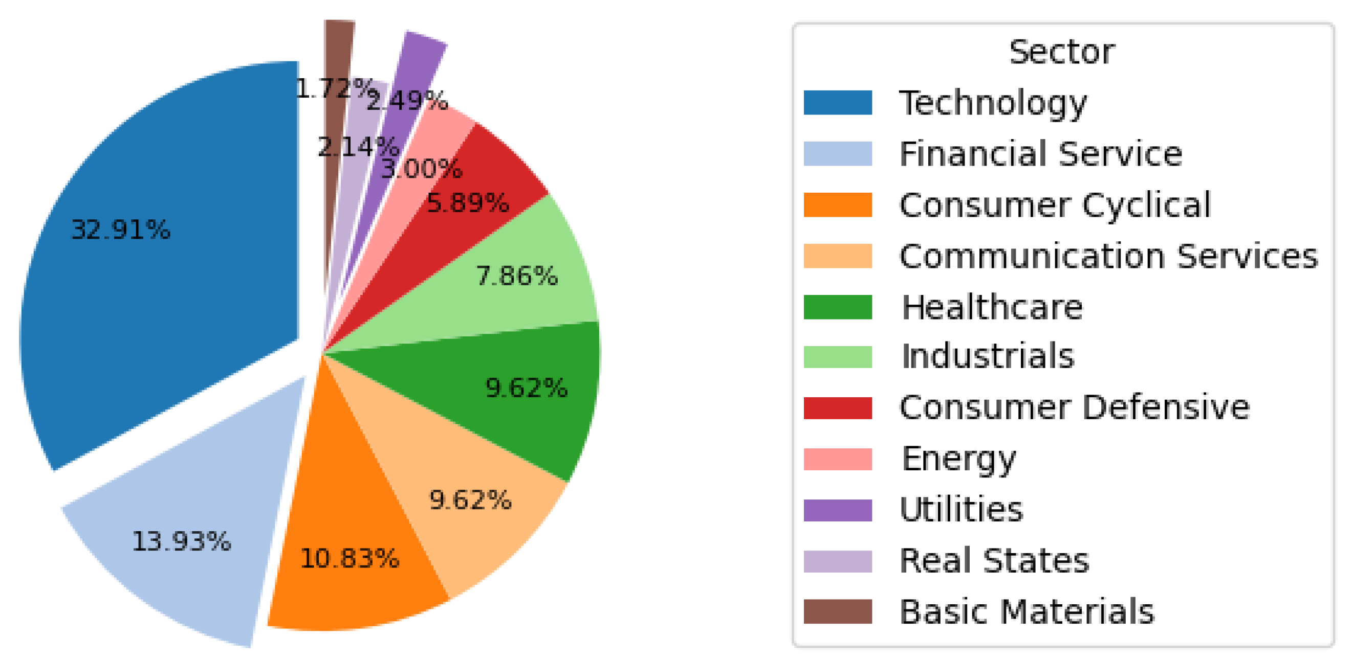
Figure 2.
Data Diagram.
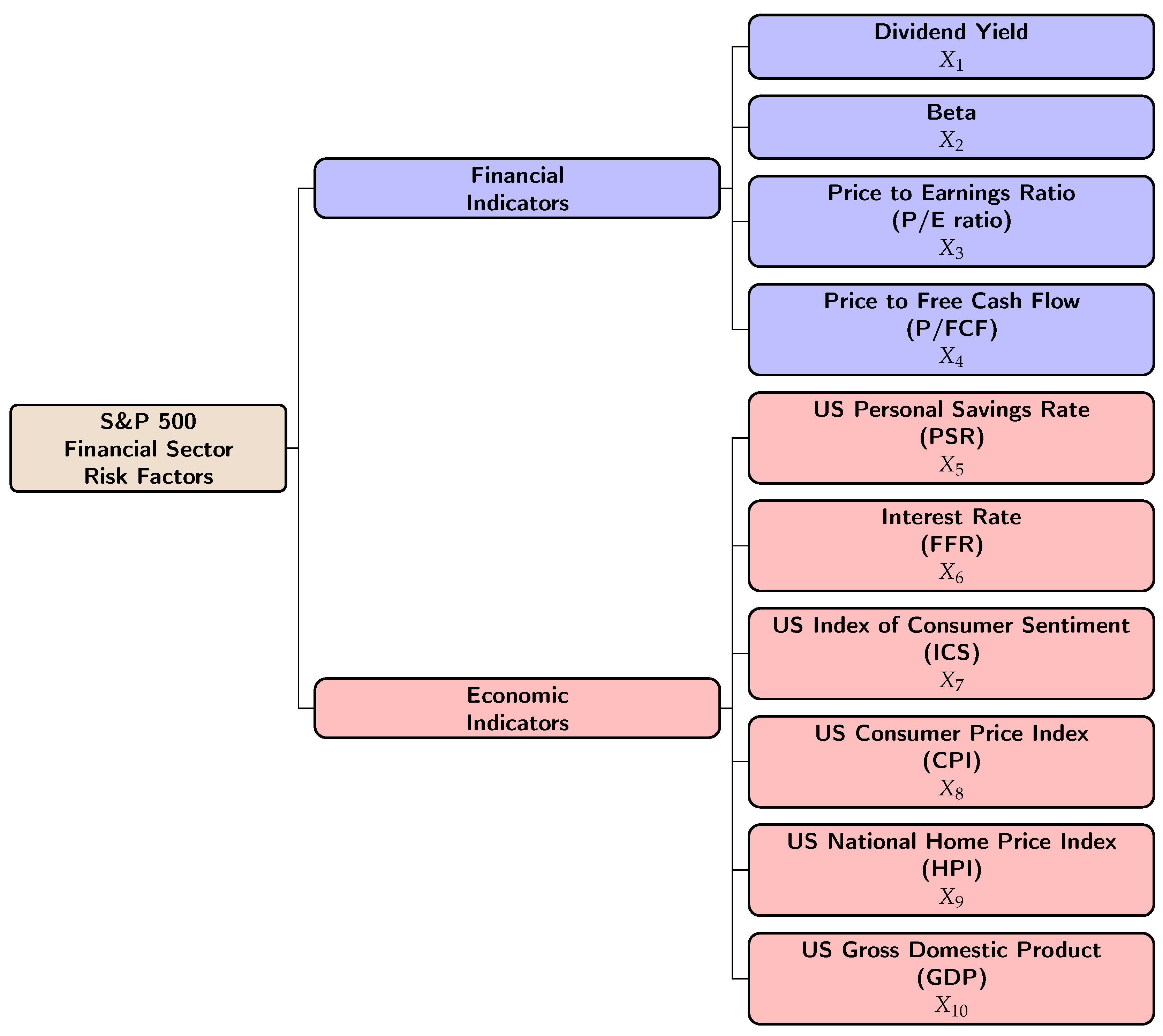
Figure 3.
Flow Chart of the Desirability Method.
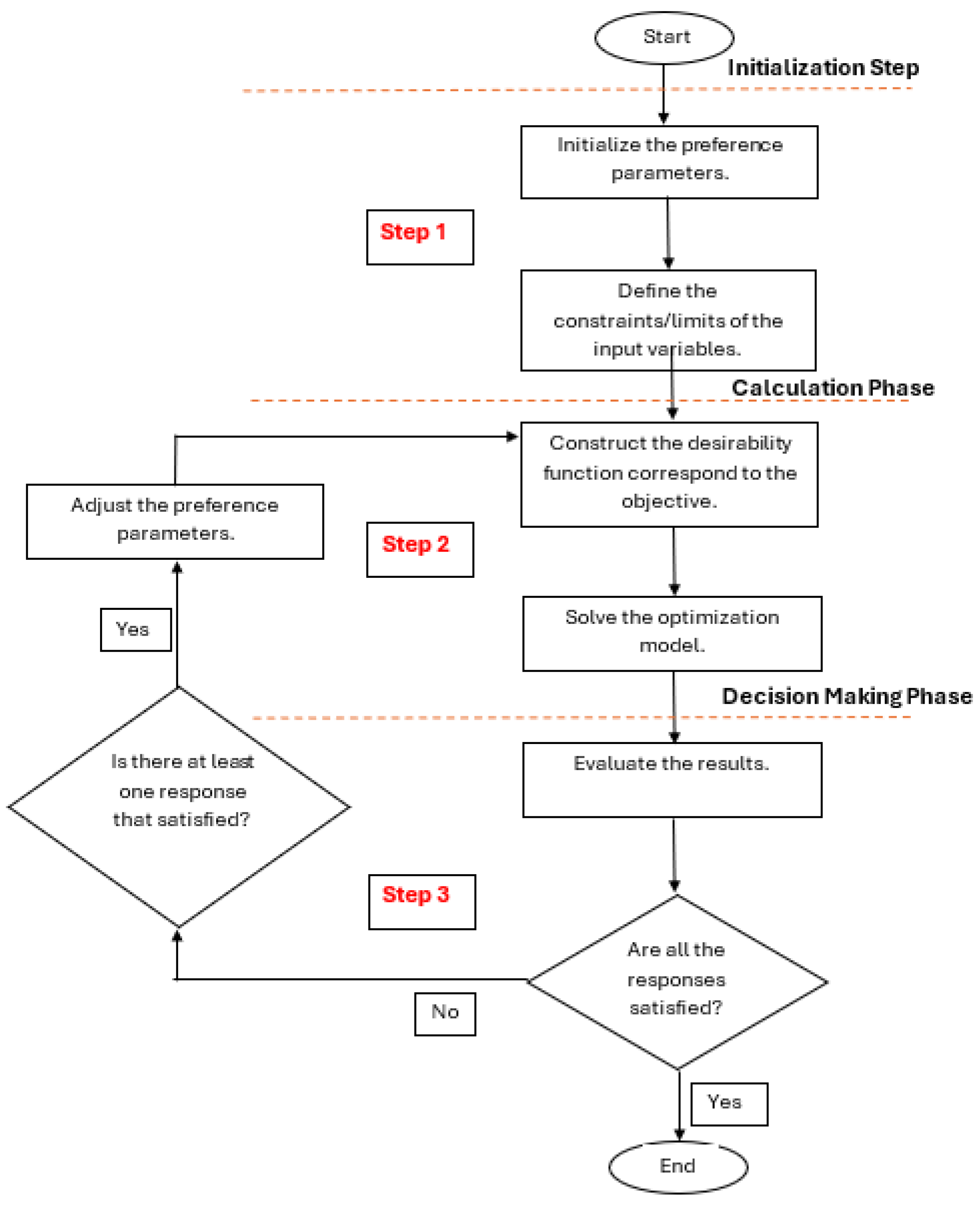
Figure 4.
Contour Plot and Surface Plot for Dividend Yield and Beta.
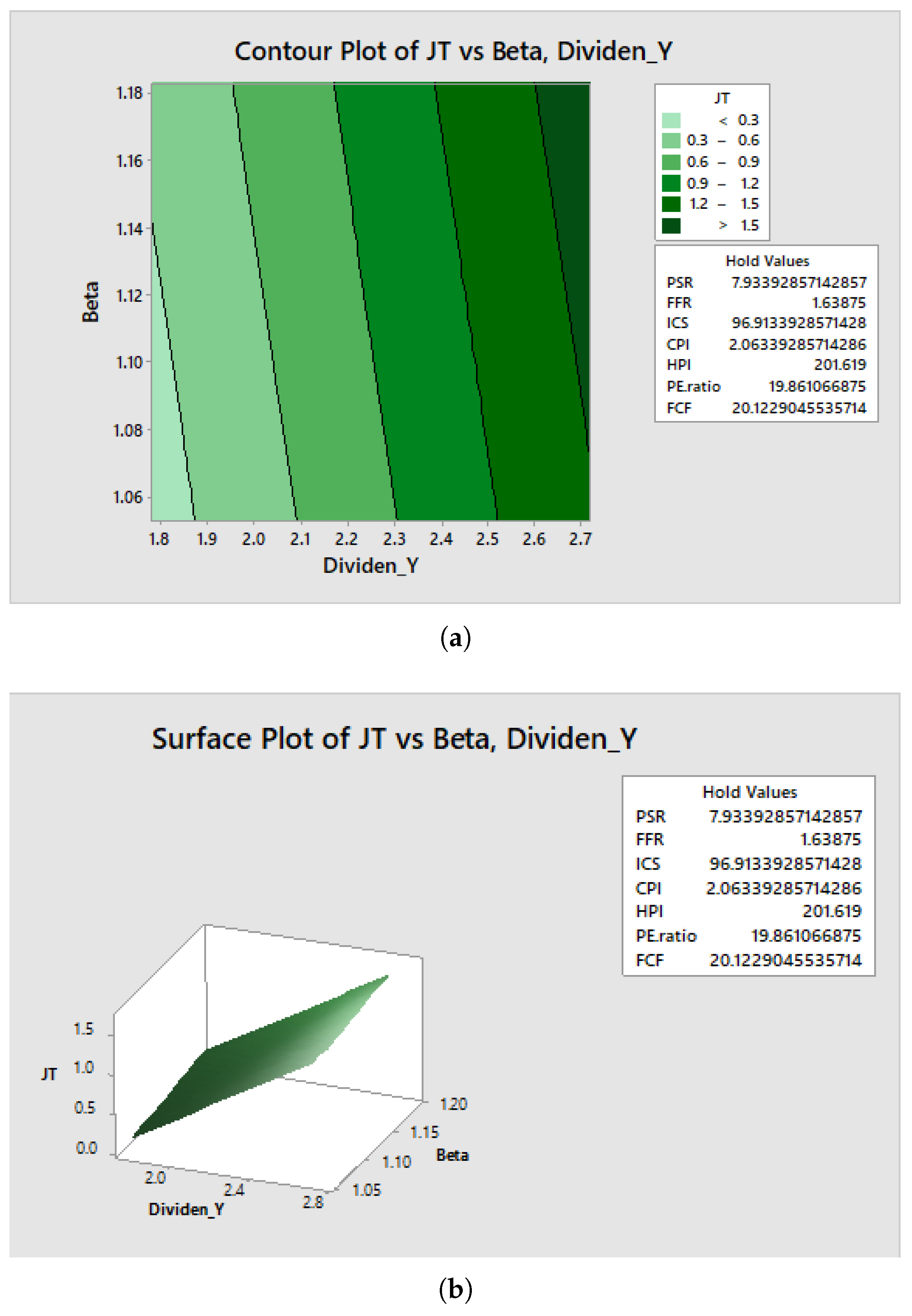
Figure 5.
Contour Plot and Surface Plot for Dividend Yield and P/E Ratio.
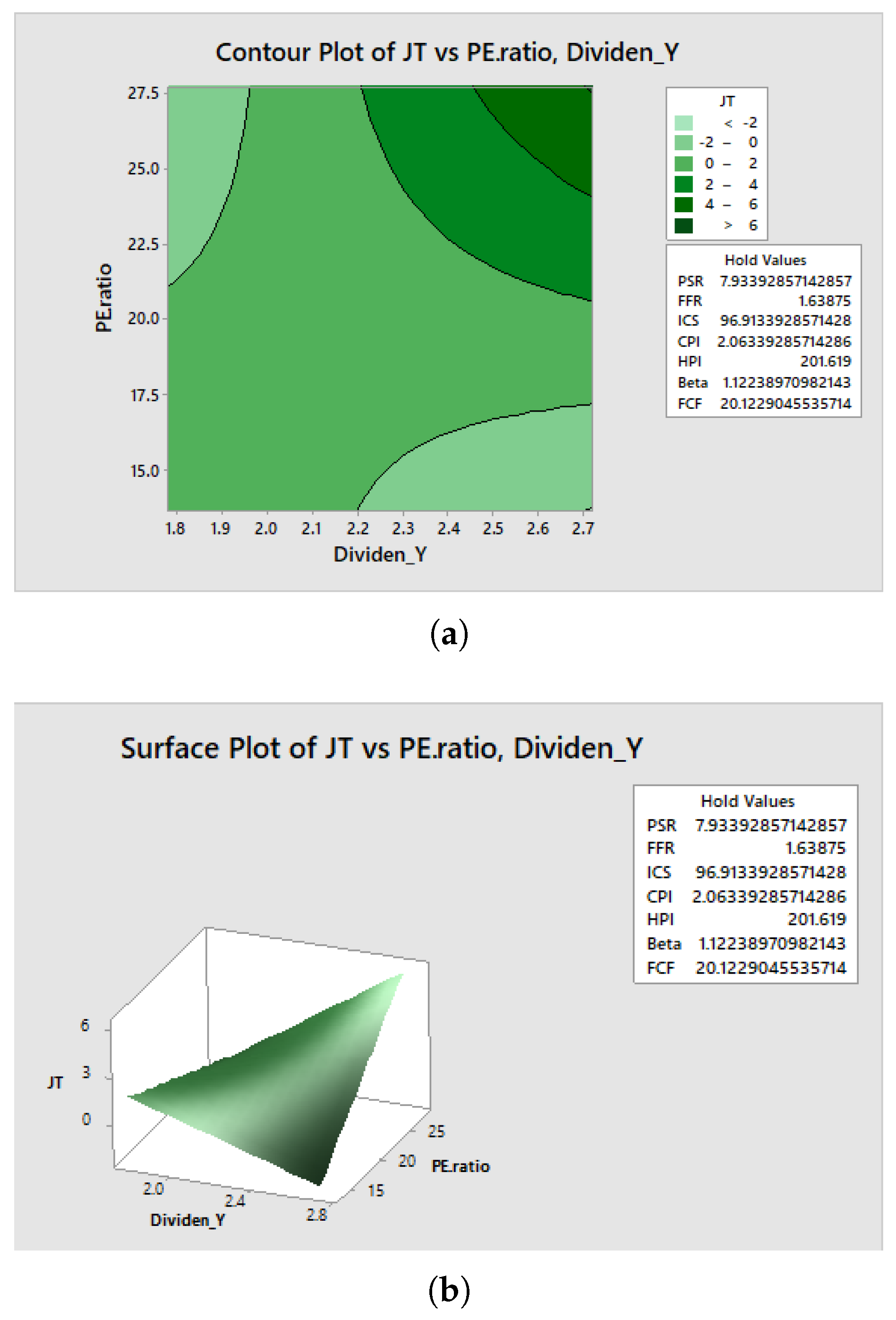
Figure 6.
Contour Plot and Surface Plot for Dividend Yield and P/E Ratio.
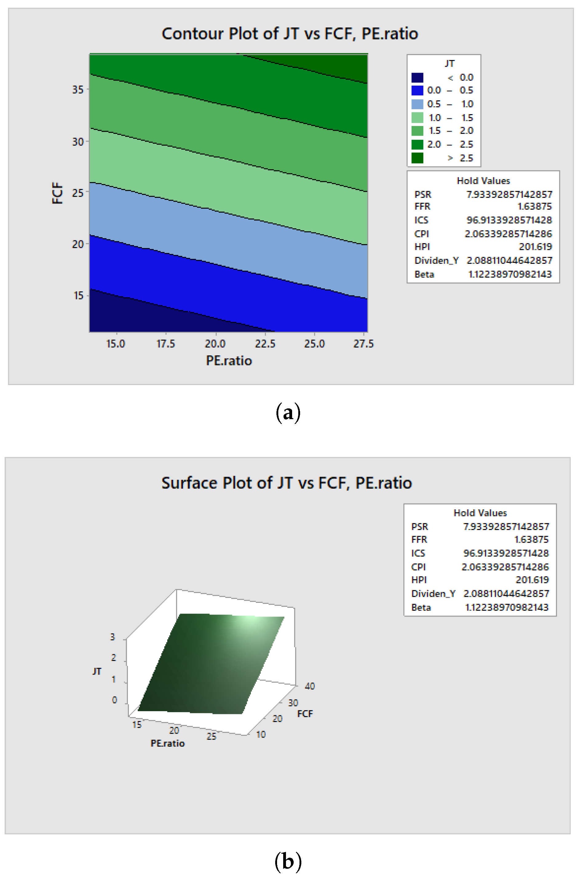

Table 1.
Constraints/Limits of the Response and Indicators.
| Indicator | Minimum | Maximum |
| -1.82063 | 2.24255 | |
| 380.38007 | 511.88997 | |
| 1.78141 | 2.71797 | |
| 1.05292 | 1.18281 | |
| 13.6510 | 27.6971 | |
| 11.4375 | 38.4019 | |
| 6.3 | 9.5 | |
| 0.66 | 2.42 | |
| 89.8 | 101.4 | |
| 1.7 | 2.4 | |
| 187.316 | 214.846 |
Table 2.
Optimal Values for the Response and Economic and Financial Indicators.
| 2.24255 | 511.88997 | 2.24969 | 1.11786 | 20.674 | 31.5997 | 7.9 | 1.54 | 95.6 | 2.05 | 201.081 |
Table 3.
Validation Results of the Optimization Process.
| SE of Fit | 95% CI | 95% PI | |||
| 0.9492 | 0.9398 | 0.99 | 0.263 | (499.859, 521.646) | (495.195, 524.504) |
Disclaimer/Publisher’s Note: The statements, opinions and data contained in all publications are solely those of the individual author(s) and contributor(s) and not of MDPI and/or the editor(s). MDPI and/or the editor(s) disclaim responsibility for any injury to people or property resulting from any ideas, methods, instructions or products referred to in the content. |
© 2025 by the authors. Licensee MDPI, Basel, Switzerland. This article is an open access article distributed under the terms and conditions of the Creative Commons Attribution (CC BY) license (http://creativecommons.org/licenses/by/4.0/).
Copyright: This open access article is published under a Creative Commons CC BY 4.0 license, which permit the free download, distribution, and reuse, provided that the author and preprint are cited in any reuse.


