
Submitted:
14 July 2025
Posted:
15 July 2025
You are already at the latest version
Abstract
A review on the development of grid technologies and corresponding numerical approaches based on lattice Boltzmann method (LBM) is performed in the present study. The history of the algorithmic development and practical applications is presented and followed by a short introduction of the basic theory of LBM, especially the classic LBGK D2Q9 model. In reality, all the different grid technologies reported aim to solve one but very important problem, the local grid refinement, which largely influences the stability, efficiency, accuracy and flexibility of the conventional LBM. The improvement of these numerical properties after employing various grid technologies is analyzed. Several grid technologies, such as body-fitted grid, multigrid, non-uniform rectangular grid, quadtree Cartesian square grid, unstructured grid and meshless discrete points, as well as the corresponding numerical approaches are compared and discussed.
Keywords:
Lattice Boltzmann method
; LBM review
; numerical approaches
; grid technology
1. Introduction
As an efficient and trustable numerical method, the lattice Boltzmann method (LBM) has been developing rapidly for roughly 40 years, this is why the numerical applications cover a wide range of engineering topics, for instance, aeronautics [1], acoustics [2], multi-phase-component flows [3], porous medium [4], rheology [5], heat and mass transfer [6], biofluids [7], magnetic fluid [8], image processing [9], crystal growth [10], and PDEs [11]. After many improvements, the methodology has progressed into a multi-functional interdisciplinary algorithm, covering subjects as fluid mechanics, mathematics, statistical mechanics, and thermal dynamics.
The prosperity of LBM undoubtedly benefits from the famous numerical lattice gas automata (LGA or FHP model), firstly introduced by Frisch et al. [12], which is usually viewed as the origin of LBM. Since it has a good performance on symmetry, it can be recovered to the Navier-Stokes equations, hence becoming an alternative solution for solving the Navier-Stokes equations. However, since the basic theory of LGA is based on the Boolean operations, it inevitably brings inconvenience and inaccuracy to the simulations. In order to improve this method, McNamara and Zanetti [13] presented the earliest lattice Boltzmann model by introducing local particle distribution functions and the Boltzmann equation to replace the Boolean operations and governing equation in LGA. This breakthrough laid the foundation of LBM, although the multi-particle collision model remained highly complex at the time, limiting its use for general numerical applications. Fortunately, Higuera and Jiménez [14] introduced the concept of the equilibrium distribution function, which was used to linearize the complex multi-particle collision model. Later, Higuera et al. [15] proposed an improved model with the enhanced collision operator to improve the numerical stability. These two models eliminated the statistical noise of the lattice gas automata and overcame the complexity of the collision operator.
Regardless of the success of the improved models [14,15] the defect inherited from LGA was still a problem needed to be solved. Chen et al. [16] advanced a single-relaxation-time model, simplifying the collision model even further, where the process to the equilibrium state was governed by a single-relaxation time. Qian et al. [17], presented the famous LBGK model based on the BGK collision theory [18], in which the complex collision term in the Boltzmann equation was further simplified. This LBGK model gradually became a very popular model for numerical applications, however, the original LBGK model suffers from the poor numerical stability whenever the single-relaxation time approaches to 0.5. As a result, many efforts have been done on improving the original LBGK models. For instance, d’Humieres [19] developed a multiple-relaxation-time LB model, where the single-relaxation time was replaced by multiple relaxation terms, considering the fact that the relaxation pace on different discrete directions are different during the streaming process. They confirmed the superior numerical stability of the multiple-relaxation-time lattice Boltzmann equation over the popular lattice BGK model. Ansumali and Karlin [20], introduced an entropic lattice Boltzmann method combined with H-theorem, where a new collision operator was introduced. When comparing with the original LBGK model, the numerical stability was improved. Montessori et al. [21] proposed a regularized lattice Boltzmann method, the core theory was to present several pre-collision distribution functions defined only in terms of macroscopic quantities, like density, linear momentum, and momentum flux tensor. Whereas, the higher-order non-equilibrium information was ignored. They proved a significant enhancement of the convergence and numerical stability of the regularized LBM over the original LBM. Dong et al. [22] presented a LES implemented LBM, advancing the original LBM to the applications of turbulence. For the Smagorinsky model, the dependence of the model coefficients on the ratio of the grid width to the Kolmogrov scale was investigated. Through numerical validations, they concluded that the LES-LBM was appropriate for turbulence simulations producing satisfactory results. Teixeira [23] optimized the LBM by incorporating k-epsilon two-equation turbulence model, improving the numerical stability of the original LBM at high Reynolds numbers. Guo et al. [24] presented a pre-conditioned LBE with an accelerated convergence rate. Compared with the original LBM, the main difference resides in the definition of equilibrium distribution functions. Numerical tests confirmed that, the convergence rate as well as the computational accuracy were enhanced. Shu et al. [25], based on the fractional step techniques proposed a fractional step LBM, in which the evolution process was split into the predictor step and the corrector step. Numerical results showed that the fractional step LBM had a good performance for the flows with high Reynolds numbers, highly improving the numerical stability of the original LBM. In order to extend the application of LBM to the compressible scenarios, Ansumali and Karlin [26] presented a consistent lattice Boltzmann method with energy conservation considered. This model was regarded as a genuine model for incompressible and weakly compressible flows, generating a valid physical model for ideal fluid. Besides, Li et al. [27] proposed a coupled double-distribution-function LBM. They proved that the model was able to be recovered to the compressible Navier-Stokes equations with a flexible specific-heat ratio and Prandtl number. An additional energy distribution function was introduced to recover the energy equation. The numerical results were found to be in excellent agreement with analytic solutions. Kang et al. [28] introduced a unified lattice Boltzmann method for flows in multiscale porous media. It was demonstrated that the method could effectively simulate flows in porous systems with varying scales, including those with coexisting multiple scales. Although the computational efficiency of LBM is quite advanced when compared with those macroscopic models, it can be even accelerated by using GPU parallel techniques [29], due to the highly parallel nature of LBM.
Considering the LBM approach, the development appears to have no limits, in fact various modified LBM models were recently presented. Ilyin [30] proposed a Gaussian LBM, where the conventional BGK equation was discretized by using a new approach. The linear streaming step and conservation of moments inherited from the original LBM were preserved in the new method, whereas the distribution function was described with a controllable error. Kellnberger et al. [31] presented a novel LBM for viscoelastic fluids to solve the problem that appears in the simulation of strongly shear-thinning fluids, where the ratio between the high-shear and low-shear viscosities is large, causing numerical stability issues in general. Fu et al. [32] focused on the volume-averaged Navier-Stokes equations in multiphase flows and introduced a pressure-based LBM. Different from the original LBM, the pressure was decoupled from density in this method. Two challenges known as the volume conservation under large pressure gradient and stability across discontinuities in void fraction were solved. Liu et al. [33] developed an enthalpy-based LBM for conjugate heat transfer, tackling the problem that the continuity of temperature and heat flux at conjugate interface is unable to be accurately enforced without special treatment. With this model, the continuity condition for temperature and heat flux on the conjugate interface can be enforced automatically without special treatment. Zhang et al. [34] presented a volumetric lattice Boltzmann method for modeling and simulating pore-scale diffusion-advection of radioactive isotopes within geopolymer porous structures, in which a concentration field of an isotope seamlessly coupled with the velocity field was introduced and simulated by the evolution of distribution functions.
Furthermore, as the artificial intelligence (AI) is nowadays booming, the development of LBM benefits a lot from it. Specifically, the emergence of AI-implemented LBM [35,36,37,38,39,40] is becoming a new trend. Generally, the studies are classified into two kinds, using LBM solutions as dataset [35,36,37,38] only to train AI models, and improving the numerical performance of original LBM [39,40], both of which accelerate the development of LBM towards a wider range of applications. Considering the improvement of LBM based on AI technology, it generally shows a great computational efficiency and accuracy over the original LBM.
The literature review reveals that LBM development has primarily emphasized numerical stability, computational accuracy, efficiency and applicability, all strongly dependent on grid structure and associated numerical algorithms. As a result, in the present review study we will mainly focus on the improvement of grid technologies related to LBM, as well as the corresponding numerical algorithms. The rest of the paper is designed as follows: section 2 introduces a brief introduction of LBM foundations, section 3 presents the different grid technologies employed and the corresponding algorithms and the paper ends with the summary of the work presented.
2. Foundations of the Conventional LBM
The Lattice Boltzmann method is a mesoscopic model which connects the microscopic movement of fluid particles and the macroscopic flow properties [41], which is originated from lattice gas automata (LGA) and then improved into the lattice Boltzmann method by replacing the lattice gas automata with the continuous Boltzmann equation, which is given by [42]
where is the distribution function, defines space vector, determines velocity vector of fluid particles, is velocity acceleration on each fluid particles, and t is the time. On the right hand side of the equation is defined as the collision term, which is a complicated integral function.
It is assumed that the flow consists of fluid particles and these particles propagate and collide continuously on a discrete mesh, simulating the macroscopic behavior of fluids. With a further development based on BGK collision theory, the Boltzmann BGK equation can be written as:
where is the BGK collision operator, is a constant, represents the discrete equilibrium distribution function and defines the discrete distribution function.
Assuming the velocity vector can be simplified into an N-dimensional limited space , the velocity discretized single-relaxation-time Boltzmann equation is written as:
where is the external force term, define the discrete velocity of fluid particles, and is the single-relaxation time.
When discretizing Equation (3) on time and space, it is obtained the single-relaxation-time discrete lattice Boltzmann BGK equation, given by:
which is the governing equation for the present study of all simulations. Based on this equation the propagation and collision process of fluid particles is accomplished, the macroscopic quantities in the fields are then calculated through distribution functions Equation (5). For instance, taking the incompressible Navier-Stokes equations as the target equation, which can be recovered from the discrete single-relaxation-time Boltzmann equation [17,42,43,44,45], the relevant macroscopic quantities, like density () and velocity (), are calculated through equilibrium distribution functions and given by:
Notice that for different target equations, the equilibrium distribution functions are constructed in different forms. Moreover, even for the same target equation, in different LBGK models, the mathematical formulas of equilibrium distribution functions could be different as well. Specifically for the popular LBGK D2Q9 model [17], the corresponding equilibrium distribution functions for a two-dimensional case are defined as:
where, is defined as the weight coefficients, represents the lattice sound speed, which is also written in terms of , where is the lattice velocity, is the grid spacing, and is the time step. The discrete velocities model is sketched in Figure 1.
3. Grid Technologies and Corresponding Algorithms
In the present study, we aim to highlight the importance of the grid considered in any simulation, which represents the discretization of the computational domain, including a real mesh or meshless discrete points. Regardless of the numerical method considered, the essence of any numerical simulation is to employ the appropriate mesh. Generally, the grid discretizes the computational domain in space, based on which, the governing equations can be solved. Regarding the numerical applications, the Navier-Stokes equations are assumed as the target equation, and in the present study, the most popular single-relaxation-time LBGK D2Q9 model is chosen to perform the grid technology analysis.
Different from the macroscopic methods, where the grid structures employed are not directly connected with governing equations, the choice of the grid in LBM simulations usually considers the specific discrete lattice velocity model in the first place, especially during the earlier stage of the LBM history. It it reasonable to think that using an appropriate grid which corresponds to the discrete lattice velocity model, the evolution process (streaming-collision) of fluid particles can be more easier and conveniently accomplished.
For example, the discrete lattice velocity LBGK D2Q7 model is sketched in Figure 2a. Indeed, with more advanced numerical models, the grid could theoretically be of any sort, however, the triangular grid presented in Figure 2b is usually the most appropriate choice for the LBGK D2Q7 model. Because only with the triangular grid, the smooth evolution process is guaranteed exactly on the grid points. Since LBGK D2Q9 model (Figure 1) is the most popular model employed in LBM numerical simulations, the corresponding grid is usually chosen as the uniform Cartesian square grid (Figure 3), which provides a good performance in most of the simulations. However, it is important to note that the numerical stability of LBGK model deteriorates whenever the single relaxation time approaches to 0.5 [41,42,43]. The relation between and the Reynolds number is given by:
where, U is the velocity, L is the characteristic length, and Re defines the Reynolds number. As can be seen from the previous equation, as Reynolds number increases to a large number, the relaxation time approaches to 0.5, at which the numerical stability is collapsed. For this reason, in order to simulate the flows at high Reynolds numbers, it is always required to use a very fine grid, having a very small value of . Besides, in some cases, the local grid refinement, adjacent to the wall boundaries, is inevitable. Yet, the grid refinement for uniform Cartesian square grid is not always a smart option, since it will cause a huge computational burden, decreasing the computational efficiency.
The dilemma scientists are trying to resolve consists in that, on one hand, the uniform Cartesian square grid perfectly fits the nature of LBGK D2Q9 model, while on the other hand, the grid refinement for the uniform Cartesian square grid is a nightmare for efficient simulations. As a result, the applications of LBM are highly restricted. In order to solve this problem, many efforts have been done to enhance the grid technologies and the corresponding algorithms, these efforts will be revealed and discussed in the remaining part of the present section.
3.1. Body-Fitted Grid
The body-fitted grid, as sketched in Figure 4, is often employed for local grid refinement along the wall boundaries with complex configurations. Inspired by the success of the body-fitted grid on the conventional computational fluid dynamics (CFD), some modified models of LBM were presented, for instance, the finite difference lattice Boltzmann method (FDLBM) [47,48,49], interpolation-supplemented lattice Boltzmann method (ISLBM) [50,51], and the Taylor series expansion and least square-based lattice Boltzmann method (TLLBM) [52].
Regarding the FDLBM, it follows the same procedure used in the conventional CFD approach, a coordinate transformation (see Figure 5) is required in the first place to transform the physical discrete domain (curvilinear system) to a computational domain (Cartesian system) through the Jacobian matrix, given by Equation (8).
where, the Jacobian is defined as . Besides, the partial derivatives of distribution functions respect to space in the original evolution (Equation (3)) are also replaced by and . Then, the evolution equation is solved by using numerical difference schemes. For example, the third order upwind scheme along horizontal direction x is given by:
Although the FDLBM with body-fitted grid is appropriate for local grid refinement, in particular for complex geometries, the computational accuracy, efficiency and numerical stability highly depend on the choice of the specific difference schemes employed. In addition, in order to maintain the second or higher order of accuracy for the method, the order of accuracy for the selected time discrete scheme should be high enough.
For the ISLBM, the coordinate transformation used in FDLBM is also considered. Yet the difference is that in FDLBM there is no evolution process at all, the governing equation is solved by using finite difference schemes, however in ISLBM, the evolution process, also known as the streaming-collision of fluid particles, is accomplished although not in the physical domain (see Figure 5), but the transformed computational domain instead (Figure 5). Since it is assumed that the flow domain can be described by a transformed computational domain with a one to one correspondence in position, where is a space vector in the physical domain. And considering that the computational domain can be projected onto a uniform Cartesian square grid. The end point of the streaming process is generally no longer a grid node regarding the body-fitted grid, an interpolation is therefore required. According to He and Doolen [50] the second-order upwind interpolation scheme is given by:
where and represent the interpolation coefficients, and define the streaming directions. Taking the discrete direction for a grid node (black dot in Figure 6) for example. The post-streaming distribution function can be calculated through the interpolation using the neighboring points (red dots in Figure 6)). Notice that all those points can be transformed into the physical domain by using Equation (8).
Regardless of the successful applications of ISLBM on simulations based on body-fitted grid, it usually brings an extra computation for both coordinate transformation and interpolation at each time step, increasing the computational costs. To the best knowledge of the present authors, the ISLBM indeed developed the LBM applications to the non-uniform irregular grid with a good numerical stability, but the computational efficiency still has room for improvement.
Furthermore, Chew et al. [52] also introduced a modified LBM for curvilinear systems, the basic purpose is the same as that presented in ISLBM, calculating the post-streaming distribution functions, which are not located exactly on the grid nodes. As described in Figure 7), the distribution function in discrete direction of the grid nodes A, B, C, D, E and P moves towards the corresponding virtual points A’, B’, C’, D’, E’, and P’, which are not located exactly on the real grid nodes. The core theory of this modified model is that, taking point P for example, the post-streaming distribution function is not obtained through the interpolations as introduced in ISLBM, instead, by using the neighboring points, a Taylor series expansion and the least square-based approximation is introduced.
3.2. Non-Uniform Rectangular Grid
In order to fulfill the purpose of local grid refinement for LBM simulations, another option of the rectangular grid is considered. When employing the grid refinement scale just around the wall boundaries, the total number of cells is reduced by about half when compared with the conventional Cartesian square grid, which to some extent, alleviates the computational burden. As a result, based on the uniform rectangular grid presented in Figure 8a, a rectangular LBM [53,54,55] was presented. A new rectangular LBGK D2Q9 model was introduced with the discrete velocities sketched in Figure 8b, where defines the grid aspect ratio. Consequently, the construction of equilibrium distribution functions are different that of the original LBGK D2Q9 model, based on which, both the multi-relaxation-time LBM [53] and single-relaxation-time LBM [54,55] models were introduced. Since the grid structure perfectly matches the streaming principle of fluid particles specifically for the rectangular LBGK D2Q9 discrete model, the evolution process is smoothly accomplished.
In reality, the rectangular grid is widely used in a more popular form, also known as the non-uniform rectangular grid, sketched in Figure 9.
Compared with the uniform rectangular grid, the non-uniform rectangular grid is more flexible for local grid refinement, further reducing the total number of cells. In reality, the present authors introduced a radial basis function implemented LBM (RBF-LBM) and a Lagrangian interpolation-based LBM (LAG-LBM). The discrete velocity model remains the same as that introduced in LBGK D2Q9 (see Figure 1). Due to the fact that the evolution can not be performed exactly on grid nodes, in other words, the post-streaming distributions remain unknown after each time step, enlighten by the ISLBM, we presented two different interpolations for approximately calculating the post-streaming distribution functions on every grid nodes. Figure 10 describes the streaming process on the non-uniform rectangular grid along a discrete direction. The interpolation scheme is constructed by using the neighboring point, as shown in Figure 10a and Figure 10b, respectively for RBF 9-bit and Lagrangian 25-bit interpolations. For the RBF-LBM, the interpolation scheme is given by:
where represents the post-streaming distribution functions of the target node , defines the interpolation function, is the general form of radial basis function, also known as the kernel function, stands for the position of the controlling point and characterizes the positions of the surrounding points. represents the Euclidean distance between two positions, is given as the coefficient of the radial basis function and M is the total number of controlling points. The interpolation scheme employed for the LAG-LBM, is given as:
Where the superscripts and respectively represent the real grid nodes and virtual nodes, and represent the interpolation coefficients.
Notice that the rectangular-based LBM is quite solid for computational accuracy and local grid refinement, however when considering the objects with curved boundaries, the grid generation becomes a bit more complicated and time-consuming. In particular, for the RBF-LBM, it remains the second-order of accuracy as the original LBGK, but converges much faster, indicating the computational efficiency is significantly improved as well.
3.3. Multigrid Technology
The multi-grid method is a mathematical algorithm for solving linear systems based on multi-grid principles. It is a numerical strategy which accelerates the convergence speed through the iterative operation among several meshes with different resolutions, for instance, the coarse grid, medium grid and fine grid. The core concept resides in the information transferring process between the coarse and fine grid, in which a coarse grid system of equations is solved initially, and then the solution is transferred to the fine grid through interpolations. Afterwards, the solution on the fine grid transfers back to the coarse grid, closing an iteration loop. The cycle finishes when the convergence is satisfied. This grid technology is suitable for improving the computational efficiency of the original LBGK based on the uniform Cartesian square grid. Actually, it has already been employed in LBM simulations, known as the multigrid LBM [58,59,60,61]. During the past few decades, the multi-grid method has seen a great progress, including many specific schemes, for instance, the V-cycle, P-cycle, W-cycle and F-cycle. Among which, the V-cycle scheme was regarded as the information transferring process from the coarse grid consecutively to the medium grid and the fine grid (prolongation), and then transfers back from the fine grid to medium and coarse grid (restriction). Numerically, the restriction and prolongation operators are respectively given by the following two equations.
where denotes the macroscopic quantities, like velocity u and density , on the grid node with coordinates of , and are coordinates on the coarse mesh, and are coordinates on the fine mesh. A full period of the classic V-cycle method is introduced in Figure 11 and Figure 12, the information on the fine grid is transferred to medium and then coarse grid through the restriction operator defined by Equation (13). While, the prolongation operation is fulfilled by using Equation (14) to transfer the information from coarse to medium and then fine grid. This procedure is repeated until a converged solution is obtained.
Indeed, with the usage of the multi-grid technology, the computational efficiency has been improved, even when using a very fine mesh, as long as the multigrid strategy is appropriately employed. The technology works fine with an acceptable accuracy for steady states, however, it fails to predict the unstable solutions with a good accuracy.
3.4. Non-Uniform Cartesian Square Grid
In order to further improve the computational efficiency of LBM based on the Cartesian square grid, apart from the multigrid technology, another efficient strategy for local grid refinement is the non-uniform Cartesian square grid, which was actually named differently in different studies, for instance, quadtree grid [62,63,64], the tree grid [65], multi-domain grid [66,67,68], multi-resolution grid [69,70], hierarchically refined grid [71], nested grid [72], and composite grid [73,74]. However the final purpose is consistent, generating the local refined Cartesian grid for LBM simulations, the difference among these studies resides in the specific methods for grid generation and the treatment of the boundary conditions on the overlapping borders between coarse and fine meshes. From Figure 13, it is observed that, although different refine strategies were employed, the grid structure is pretty much similar, serving for the same purpose.
Since the entire computational domain is divided into many sub-domains with different grid levels (grid spacing), the grid consists of the staggered coarse and fine grid. The overlapping borders belongs to both, the fine and coarse grid, which is regarded as the interface of information exchange between these two grids and need to be treated specially. This treatment usually requires a spatial interpolation scheme with high order of accuracy. It is to be noted that the values of grid spacing for coarse and fine grids are different. A generic mathematical expression relating two grid spacings reads as.
Which means that during one time step, the distribution functions evolve twice on the fine grid with grid spacing , but only once on the coarse grid with grid spacing . Since it is assumed in general that , which is an enforced condition, we can be certain that the evolution is to be accomplished exactly on the finest grid nodes. As a result, when considering the interpolation along the overlapping borders, it must be performed with the same timing for both coarse and fine grid.
It was evaluated that with the employment of the non-uniform Cartesian square grid, the computational efficiency was highly increased, it was about 20 times faster than that of the original LBM for a given case and using the same equipment, the computational accuracy was excellent. Besides, the non-uniform Cartesian square grid is applicable for any kind of complex geometries, which makes the LBM applications even more convenient and plausible. However, due to the existence of the overlapping borders, on which the serrations of contours out of the discontinuity are observed, see the marked red box in Figure 14, the non-uniform Cartesian square grid can be employed in limited applications.
3.5. Unstructured Grid
As LBM quickly develops, apart from the efforts to effectively use the Cartesian grid, many scholars have tried to extend the conventional LBM to unstructured grid. Since the structured grid (uniform Cartesian square grid) has a natural limitation for practical engineering applications with complex geometries, in particular a grid refinement adjacent to the wall boundaries [74]. Besides, in the conventional LBM, the discretizations for moment velocity and space are coupled with each other, which can be clearly seen in Figure 2 and Figure 3. But in reality, these discretizatoins do not necessarily have to be coupled [75]. Hence, a finite volume LBM [76,77,78,79,80,81,82] based on unstructured grid emerge as a requirement. For this method, the unstructured grid usually consists of triangle or polygon elements, as respectively shown in Figure 15a and Figure 15b.
Among all these studies, Peng et al. [77] presented a finite volume LBM, which is regarded as the first improved approach in which the grid is really free of structure form [76]. Based on these excellent studies [76,77,78,79,80,81,82,83,84,85], the consistent development the finite volume LBM method has been performed. Notice that in these studies, the classic LBGK D2Q9 model was usually used for velocity discretization and the space was discretized based on, generally two approaches, the cell-vertex scheme [76,77,78,79,80,81,82,83] and the median-dual scheme [84,85]. Taking for example, the cell-vertex scheme with the triangle element, it is observed that the triangular elements surround an interior node (centroid) of the grid, on which the flow variables are arranged, as sketched in Figure 16. Regarding the construction for the finite volume LBM, no further elaboration will be provided in present study, since the detailed information has already been introduced in the literature [76,77,78,79,80,81,82,83,84,85]. Notice that with the prosperity of the finite volume LBM, the applicability of LBM simulations was further extended, since the unstructured grid shows a great adaption for complex geometries, especially with curved boundaries. Besides, the grid refinement can be perfectly performed on the wall boundaries, maintaining the computational efficiency as good as that of the non-uniform Cartesian square grid.
Furthermore, another option known as finite element lattice Boltzmann method [86,87,88], was introduced for unstructured grids, which also increases the flexibility of LBM with an acceptable computational efficiency and accuracy. The core theory is that the governing equation (Equation (4)) without the external force term can be split into two separate parts, streaming and collision, and are given by:
Due to the fact the collision process is performed locally, there is no need to involve unstructured grid, whereas the streaming must be discretized on an unstructured grid. As a result, the entire evolution is accomplished with two steps, streaming and collision, are calculated separately.
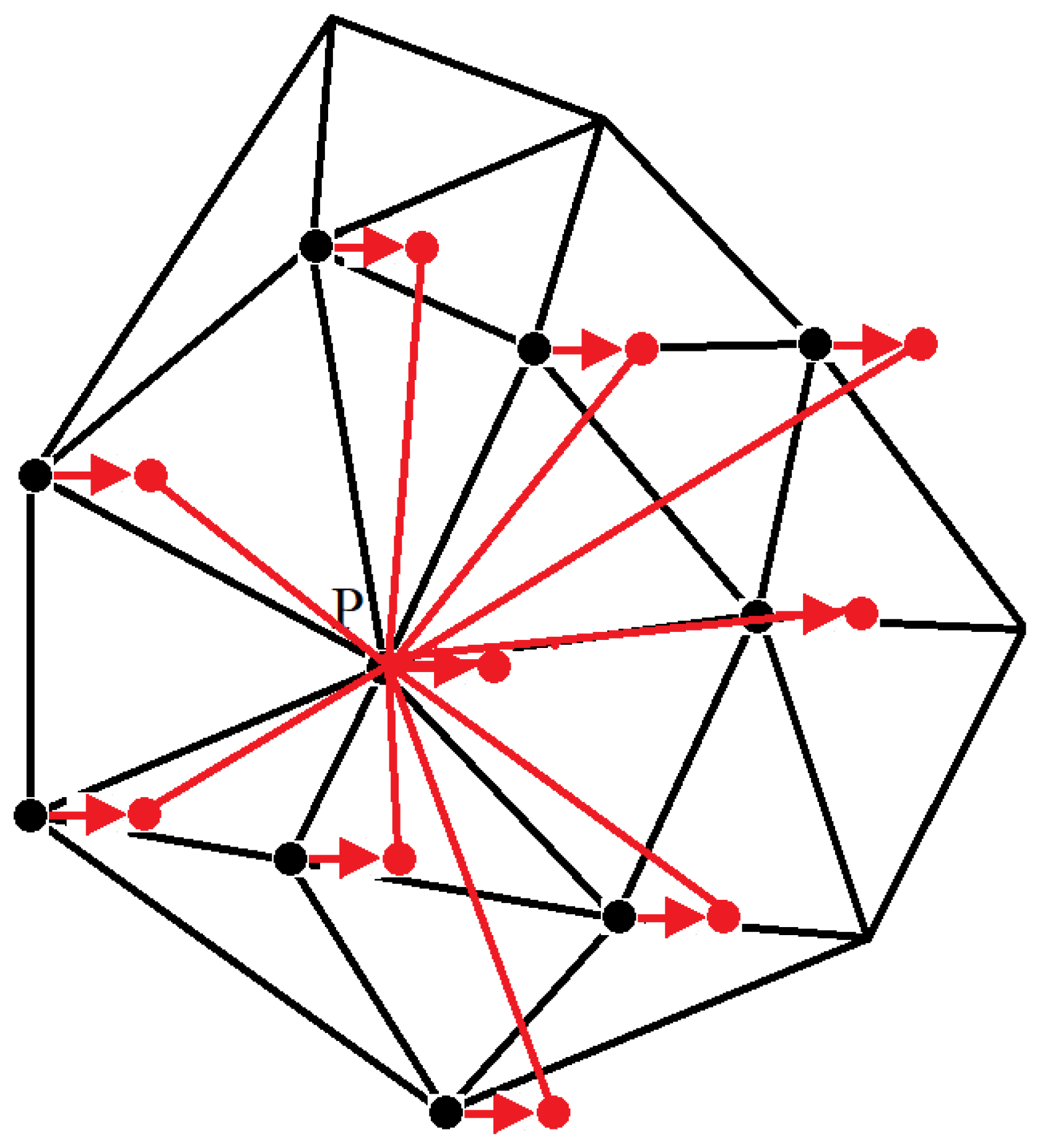
Notice as well that, based on the theory of RBF-LBM [56] introduced by the present authors, the improved RBF-LBM, can also be applied to the unstructured grid and meshless methods. The main idea is the same as that used in RBF-LBM, suggesting that after the streaming process, the distribution functions (red arrows in Figure 17) on the grid node (black dots in Figure 17), stream to the virtual points (red dots in Figure 17). By calculating the Euclidean distance (red line segments in Figure 17), the neighboring points needed for the interpolation are allocated. In reality, we choose the 9 neighboring points most close to the target grid node P, forming a 9-bit RBF interpolation for approximately predicting the distribution functions.
3.6. Meshless
Following the same idea, consisting in decoupling the velocity and space discretizations, the meshless lattice Boltzmann method [89,90,91,92,93] was introduced. When compared with the unstructured grid LBM, the difference is that instead using a grid, the discrete points are directly employed for simulations.
Figure 18.
Meshless computational domain with discrete points [92].
Figure 18.
Meshless computational domain with discrete points [92].
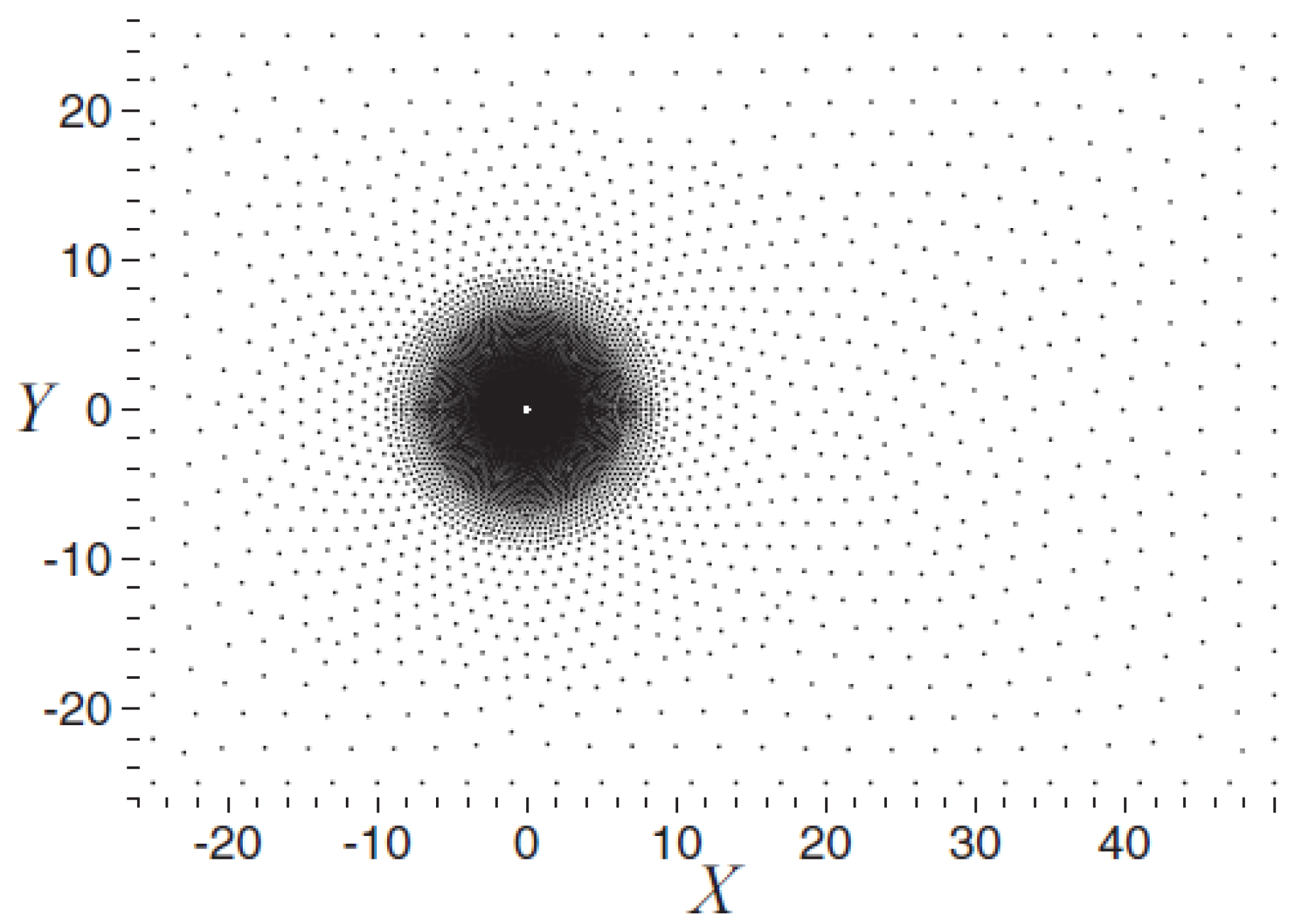
Based on Taylor series expansion and least square method, Shu et al. [89] presented a modified LBM which according to the authors, shows a remarkable computational efficiency. The basic theory is the same as the one introduced in their investigation [52] in Section 3.1, suggesting that the post-streaming distribution functions which do not exactly fit on the grid nodes are approximately obtained through Taylor series expansion combined with the least square method. Based on the RBF interpolation, Strzelczyk and Matyka [90] also introduced a meshless LBM to simulate the evolution equation on the discrete points. The basic idea is exactly the same as that introduced by the present authors when dealing with the non-uniform rectangular grid and unstructured grid. It was concluded that the meshless LBM based on RBF has a better performance when considering the convergence. Bardow et al. [91], introduced a multispeed meshless LBM, in which the discrete velocities were obtained from minimization of the entropy function H with mass and momentum conservation applied. Since the meshless lattice Boltzmann methods are not restricted to rational-number ratios between discrete velocities, the exact Hermite models along with their rational-number approximations can be directly used in the design of the meshless LBM. It was proved that the computational accuracy was improved by using the multispeed model. The method presented by Musavi and Ashrafizaadeh [92,93] is regarded as the simplification of the finite element LBM, where the evolution equation was solved separately with two steps, streaming and collision. The space was discretized by using local Petrov-Galerkin scheme and the time was discretized by using the Lax-Wendroff scheme. Obviously, the meshless LBM further increases the flexibility of LBM, whereas the numerical procedure is relatively a bit simpler than that of the unstructured grid LBM.
4. Summary
In this paper, a review on the grid technologies and the corresponding algorithms under the framework of lattice Boltzmann method is presented. In order to improve the numerical accuracy, efficiency, stability and flexibility, different grid strategies along with the modified approaches were proposed.
Although the body-fitted grid is perfect for local grid refinement especially for complex curved boundaries and the corresponding methods, like finite difference LBM and interpolation supplemented LBM are proved to be solid, the computational accuracy and stability highly depends on the differential schemes, which leads to a poor performance for generic applications. In addition, the extra computation on coordinate transformation and interpolation somehow decreases the computational efficiency.
The multigrid technology works appropriately for steady states with a faster convergence speed, however, it fails to deal with the unstable solutions.
The non-uniform rectangular grid could alleviate the computational burden to some extent with a relatively good performance on local grid refinement, and the corresponding methods are trustable. Regardless of the fact that the extra interpolation process increases the computational workload, the total number of cells is under control, maintaining a satisfactory computational efficiency as good as in other methodologies. But it is not convenient for complex geometries with curved boundaries.
The quadtree grid is capable of highly increasing the computational efficiency of LBM with a trustable computational accuracy. Meanwhile, it is perfect for local grid refinement even with complex curved geometries. In addition, the physical background is relatively simple and easy for coding. However, the election of the interpolation schemes for information exchange along the overlapping borders must be prudent.
The unstructured grid endues a remarkable flexibility to LBM, improving the generalization of LBM to an unprecedented level. Yet, the complicated physical background of finite volume LBM and finite element LBM usually brings a more complex numerical process, which is difficult for coding and relatively more time-consuming over the non-uniform Cartesian square grid-based LBM. Regarding the meshless LBM, the advantages achieved through the unstructured grid LBM are even extended.
Anyhow, all these methods are recognized as reliable numerical approaches for simulations with engineering purposes, as long as the chosen method is appropriate to the given problem.
With the fast development during the last few decades, it seems that the improvement on novelty of new approaches nearly reaches to a limit. Whereas, as the technology of artificial intelligence is nowadays booming, the great breakthrough in LBM for the next ten years could possibly happen in the research of AI supplemented LBM.
Author Contributions
Conceptualization, B.A.; methodology, B.A. and K.D.C; formal analysis, B.A., K.D.C and J.M.B.; investigation, B.A. and K.D.C; data curation, B.A.and K.D.C; writing—original draft preparation, B.A., K.D.C and J.M.B. writing—review and editing, B.A. and J.M.B.; visualization, B.A., K,D.C. and J.M.B.; supervision, B.A. and J.M.B.; project administration, B.A. and J.M.B. All authors have read and agreed to the published version of the manuscript.
Funding
This research was founded by the project provided by the Northwestern Polytechnical University (G2024 KY0613). The present research is also supported by the project (20230013053008) provided by Aeronautical Science Foundation of China and by the Spanish Ministerio de Ciencia, Innovacion y Universidades with the project PID2023-150014OB-C21.
Institutional Review Board Statement
Not applicable.
Informed Consent Statement
Not applicable.
Data Availability Statement
The original contributions presented in the study are included in the article, further inquiries can be directed to the corresponding author.
Conflicts of Interest
The authors declare no conflicts of interest.
References
- Song, Y.; Yang, L.; Du, Y.; Xiao, Y.; Shu, C. Double distribution function-based lattice Boltzmann flux solver for simulation of compressible viscous flows. Physics of Fluids 2024, 36. [CrossRef]
- Bocanegra, J.A.; Misale, M.; Borelli, D. A systematic literature review on Lattice Boltzmann Method applied to acoustics. Engineering Analysis with Boundary Elements 2024, 158, 405–429. [CrossRef]
- Qiao, Z.; Yang, X.; Zhang, Y. A free-energy based multiple-distribution-function lattice Boltzmann method for multi-component and multi-phase flows. Applied Thermal Engineering 2024, 257, 124241. [CrossRef]
- Kefayati, G. Integration of vorticity–velocity formulation in a lattice Boltzmann method for porous media. Physics of Fluids 2024, 36. [CrossRef]
- Hill, B.; Mitchell, T.; Aminossadati, S.; Leonardi, C.; et al. Development and validation of a phase-field lattice Boltzmann method for non-Newtonian Herschel-Bulkley fluids in three dimensions. Computers & Mathematics with Applications 2024, 176, 398–414. [CrossRef]
- Wu, S.; Zhu, K.; Liu, X.; Huang, Y. Lattice Boltzmann model combined with immersed boundary method for two-dimensional radiative heat transfer with irregular geometries. International Journal of Thermal Sciences 2024, 203, 109170. [CrossRef]
- Vaseghnia, H.; Jettestuen, E.; Teigen Giljarhus, K.E.; Vinningland, J.L.; Hiorth, A. Effects of hematocrit and non-Newtonian blood rheology on pulsatile wall shear stress distributions in vascular anomalies: A multiple relaxation time lattice Boltzmann approach. Physics of Fluids 2024, 36. [CrossRef]
- Li, J.; Chua, K.T.E.; Li, H.; Nguyen, V.T.; Wise, D.J.; Xu, G.X.; Kang, C.W.; Chan, W.H.R. On the consistency of three-dimensional magnetohydrodynamical lattice Boltzmann models. Applied Mathematical Modelling 2024, 132, 751–765. [CrossRef]
- Chen, Y.; Lu, D.; Courbebaisse, G. A parallel image registration algorithm based on a lattice Boltzmann model. Information 2019, 11, 1. [CrossRef]
- Chai, S.; Ren, Z.; Ji, S.; Zheng, X.; Zhou, L.; Zhang, L.; Ji, X. Exploring the Influence of Solvation on Multidimensional Particle Size Distribution Based on the Spiral Growth Model and the Lattice Boltzmann Method. Industrial & Engineering Chemistry Research 2024, 63, 20633–20650. [CrossRef]
- An, B.; Bergadà, J. A 8-neighbor model lattice Boltzmann method applied to mathematical–physical equations. Applied Mathematical Modelling 2017, 42, 363–381. [CrossRef]
- Frisch, U.; Hasslacher, B.; Pomeau, Y. Lattice-gas automata for the Navier-Stokes equation. Physical review letters 1986, 56, 1505. [CrossRef]
- McNamara, G.R.; Zanetti, G. Use of the Boltzmann equation to simulate lattice-gas automata. Physical review letters 1988, 61, 2332. [CrossRef]
- Higuera, F.J.; Jiménez, J. Boltzmann approach to lattice gas simulations. Europhysics letters 1989, 9, 663. [CrossRef]
- Higuera, F.; Succi, S.; Benzi, R. Lattice gas dynamics with enhanced collisions. Europhysics letters 1989, 9, 345. [CrossRef]
- Chen, S.; Chen, H.; Martnez, D.; Matthaeus, W. Lattice Boltzmann model for simulation of magnetohydrodynamics. Physical Review Letters 1991, 67, 3776. [CrossRef]
- Qian, Y.H.; d’Humières, D.; Lallemand, P. Lattice BGK models for Navier-Stokes equation. Europhysics letters 1992, 17, 479. [CrossRef]
- Bhatnagar, P.L.; Gross, E.P.; Krook, M. A model for collision processes in gases. I. Small amplitude processes in charged and neutral one-component systems. Physical review 1954, 94, 511. [CrossRef]
- d’Humières, D. Multiple–relaxation–time lattice Boltzmann models in three dimensions. Philosophical Transactions of the Royal Society of London. Series A: Mathematical, Physical and Engineering Sciences 2002, 360, 437–451.
- Ansumali, S.; Karlin, I.V. Entropy function approach to the lattice Boltzmann method. Journal of Statistical Physics 2002, 107, 291–308. [CrossRef]
- Montessori, A.; Falcucci, G.; Prestininzi, P.; La Rocca, M.; Succi, S. Regularized lattice Bhatnagar-Gross-Krook model for two-and three-dimensional cavity flow simulations. Physical Review E 2014, 89, 053317. [CrossRef]
- Dong, Y.H.; Sagaut, P.; Marie, S. Inertial consistent subgrid model for large-eddy simulation based on the lattice Boltzmann method. Physics of Fluids 2008, 20. [CrossRef]
- Teixeira, C.M. Incorporating turbulence models into the lattice-Boltzmann method. International Journal of Modern Physics C 1998, 9, 1159–1175. [CrossRef]
- Guo, Z.; Zhao, T.; Shi, Y. Preconditioned lattice-Boltzmann method for steady flows. Physical Review E—Statistical, Nonlinear, and Soft Matter Physics 2004, 70, 066706. [CrossRef]
- Shu, C.; Niu, X.; Chew, Y.T.; Cai, Q. A fractional step lattice Boltzmann method for simulating high Reynolds number flows. Mathematics and Computers in Simulation 2006, 72, 201–205. [CrossRef]
- Ansumali, S.; Karlin, I.V. Consistent lattice Boltzmann method. Physical review letters 2005, 95, 260605.
- Li, Q.; He, Y.; Wang, Y.; Tao, W. Coupled double-distribution-function lattice Boltzmann method for the compressible Navier-Stokes equations. Physical Review E—Statistical, Nonlinear, and Soft Matter Physics 2007, 76, 056705. [CrossRef]
- Kang, Q.; Zhang, D.; Chen, S. Unified lattice Boltzmann method for flow in multiscale porous media. Physical Review E 2002, 66, 056307. [CrossRef]
- Kaufman, A.; Fan, Z.; Petkov, K. Implementing the lattice Boltzmann model on commodity graphics hardware. Journal of Statistical Mechanics: Theory and Experiment 2009, 2009, P06016. [CrossRef]
- Ilyin, O. Gaussian Lattice Boltzmann method and its applications to rarefied flows. Physics of Fluids 2020, 32. [CrossRef]
- Kellnberger, R.; Jüngst, T.; Gekle, S. Novel lattice Boltzmann method for simulation of strongly shear thinning viscoelastic fluids. International Journal for Numerical Methods in Fluids 2024. [CrossRef]
- Fu, S.; Hao, Z.; Wang, L. A pressure-based lattice Boltzmann method for the volume-averaged Navier-Stokes equations. Journal of Computational Physics 2024, 516, 113350. [CrossRef]
- Liu, X.; Tong, Z.X.; He, Y.L.; Du, S.; Li, M.J. Enthalpy-based cascaded lattice Boltzmann method for conjugate heat transfer. International Communications in Heat and Mass Transfer 2024, 159, 107956. [CrossRef]
- Zhang, X.; Mao, Z.; Hilty, F.W.; Li, Y.; Grandjean, A.; Montgomery, R.; zur Loye, H.C.; Yu, H.; Hu, S. Volumetric lattice Boltzmann method for pore-scale mass diffusion-advection process in geopolymer porous structures. Journal of Rock Mechanics and Geotechnical Engineering 2024. [CrossRef]
- Xu, S.; Wang, H.; Qu, Z. Deep learning assisting construction of heat transfer constitutive relationships for porous media. International Journal of Heat and Fluid Flow 2024, 110, 109591. [CrossRef]
- Kang, Q.; Li, K.Q.; Fu, J.L.; Liu, Y. Hybrid LBM and machine learning algorithms for permeability prediction of porous media: A comparative study. Computers and Geotechnics 2024, 168, 106163. [CrossRef]
- Ren, F.; Ding, Z.; Zhao, Y.; Song, D. Active control of wake-induced vibration using deep reinforcement learning. Physics of Fluids 2024, 36. [CrossRef]
- Zhao, F.; Zhou, Y.; Ren, F.; Tang, H.; Wang, Z. Mitigating the lift of a circular cylinder in wake flow using deep reinforcement learning guided self-rotation. Ocean Engineering 2024, 306, 118138. [CrossRef]
- Wang, Z.; Xu, Y.; Zhang, Y.; Ke, Z.; Tian, Y.; Zhao, S. An accelerated lattice Boltzmann method for natural convection coupled with convolutional neural network. Physics of Fluids 2024, 36. [CrossRef]
- Zhuang, Z.; Xu, Q.; Zeng, H.; Pan, Y.; Wen, B. A deep-learning-based compact method for accelerating the electrowetting lattice Boltzmann simulations. Physics of Fluids 2024, 36. [CrossRef]
- Succi, S. The lattice Boltzmann equation: for fluid dynamics and beyond; Oxford university press, 2001.
- He, Y.; Wang, Y.; Li, Q.; et al. Lattice Boltzmann method: theory and applications. Science, Beijing 2009.
- Guo, Z.L.; Zheng, C.; et al. Theory and applications of lattice Boltzmann method. Science, Beijing 2009, 1.
- Chen, H.; Chen, S.; Matthaeus, W.H. Recovery of the Navier-Stokes equations using a lattice-gas Boltzmann method. Physical review A 1992, 45, R5339. [CrossRef]
- Ladd, A.J. Numerical simulations of particulate suspensions via a discretized Boltzmann equation. Part 1. Theoretical foundation. Journal of fluid mechanics 1994, 271, 285–309. [CrossRef]
- Nabovati, A.; Sellan, D.P.; Amon, C.H. On the lattice Boltzmann method for phonon transport. Journal of Computational Physics 2011, 230, 5864–5876. [CrossRef]
- Mei, R.; Shyy, W. On the finite difference-based lattice Boltzmann method in curvilinear coordinates. Journal of Computational Physics 1998, 143, 426–448. [CrossRef]
- Tölke, J.; Krafczyk, M.; Schulz, M.; Rank, E. Discretization of the Boltzmann equation in velocity space using a Galerkin approach. Computer physics communications 2000, 129, 91–99. [CrossRef]
- Seta, T.; Kono, K.; Martinez, D.; Chen, S. Lattice Boltzmann scheme for simulating two-phase flows. JSME International Journal Series B Fluids and Thermal Engineering 2000, 43, 305–313.
- He, X.; Doolen, G. Lattice Boltzmann method on curvilinear coordinates system: flow around a circular cylinder. Journal of Computational Physics 1997, 134, 306–315. [CrossRef]
- Mirzaei, M.; Poozesh, A. Simulation of fluid flow in a body-fitted grid system using the lattice Boltzmann method. Physical Review E—Statistical, Nonlinear, and Soft Matter Physics 2013, 87, 063312. [CrossRef]
- Chew, Y.; Shu, C.; Niu, X. Simulation of unsteady incompressible flows by using Taylor series expansion-and least square-based lattice Boltzmann method. International Journal of Modern Physics C 2002, 13, 719–738. [CrossRef]
- Bouzidi, M.; d’Humières, D.; Lallemand, P.; Luo, L.S. Lattice Boltzmann equation on a two-dimensional rectangular grid. Journal of Computational Physics 2001, 172, 704–717. [CrossRef]
- Peng, C.; Guo, Z.; Wang, L.P. A lattice-BGK model for the Navier–Stokes equations based on a rectangular grid. Computers & Mathematics with Applications 2019, 78, 1076–1094. [CrossRef]
- Yahia, E.; Premnath, K.N. Central moment lattice Boltzmann method on a rectangular lattice. Physics of Fluids 2021, 33. [CrossRef]
- Hu, X.; Bergadà, J.; Li, D.; Sang, W.; An, B. A modified lattice Boltzmann approach based on radial basis function approximation for the non-uniform rectangular mesh. International Journal for Numerical Methods in Fluids 2024, 96, 1695–1714. [CrossRef]
- Bo, A.; Xinyu, M.; Shuangjun, Y.; Weimin, S. RESEARCH ON THE LATTICE BOLTZMANN ALGORITHM FOR GRID REFINEMENT BASED ON NON-UNIFORM RECTANGULAR GRID. Chinese Journal of Theoretical and Applied Mechanics 2023, 55, 2288–2296.
- Tölke, J.; Krafczyk, M.; Rank, E. A multigrid-solver for the discrete Boltzmann equation. Journal of Statistical Physics 2002, 107, 573–591. [CrossRef]
- Mavriplis, D.J. Multigrid solution of the steady-state lattice Boltzmann equation. Computers & fluids 2006, 35, 793–804. [CrossRef]
- Armstrong, C.; Peng, Y. An mrt extension to the multigrid lattice Boltzmann method. Communications in Computational Physics 2019, 26, 1178–1195. [CrossRef]
- An, B.; Bergadà, J.M.; Sang, W.M. A simplified new multigrid algorithm of lattice Boltzmann method for steady states. Computers & Mathematics with Applications 2023, 135, 102–110. [CrossRef]
- Chen, Y.; Kang, Q.; Cai, Q.; Zhang, D. Lattice Boltzmann method on quadtree grids. Physical Review E—Statistical, Nonlinear, and Soft Matter Physics 2011, 83, 026707. [CrossRef]
- ElSherbiny, A.; Leclaire, S. Integration of Lattice Boltzmann-overset method with non-conforming quadtree mesh based on the combination of spatial and Lagrangian-link interpolated streaming technique. Computers & Fluids 2025, 289, 106522. [CrossRef]
- Cheng, Z.; Wachs, A. An immersed boundary/multi-relaxation time lattice Boltzmann method on adaptive octree grids for the particle-resolved simulation of particle-laden flows. Journal of Computational Physics 2022, 471, 111669. [CrossRef]
- An, B.; Bergadà, J.M.; Mellibovsky, F.; Sang, W. New applications of numerical simulation based on lattice Boltzmann method at high Reynolds numbers. Computers & Mathematics with Applications 2020, 79, 1718–1741. [CrossRef]
- Pellerin, N.; Leclaire, S.; Reggio, M. An implementation of the Spalart–Allmaras turbulence model in a multi-domain lattice Boltzmann method for solving turbulent airfoil flows. Computers & Mathematics with Applications 2015, 70, 3001–3018. [CrossRef]
- Falagkaris, E.; Ingram, D.M.; Viola, I.M.; Markakis, K. PROTEUS: A coupled iterative force-correction immersed-boundary multi-domain cascaded lattice Boltzmann solver. Computers & Mathematics with Applications 2017, 74, 2348–2368. [CrossRef]
- Dorschner, B.; Chikatamarla, S.S.; Karlin, I.V. Transitional flows with the entropic lattice Boltzmann method. Journal of Fluid Mechanics 2017, 824, 388–412. [CrossRef]
- Touil, H.; Ricot, D.; Lévêque, E. Direct and large-eddy simulation of turbulent flows on composite multi-resolution grids by the lattice Boltzmann method. Journal of Computational Physics 2014, 256, 220–233. [CrossRef]
- He, Z.W.; Shu, C.; Chen, Z. Simplified lattice Boltzmann method on multi-resolution mesh. Physics of Fluids 2024, 36. [CrossRef]
- Eitel-Amor, G.; Meinke, M.; Schröder, W. A lattice-Boltzmann method with hierarchically refined meshes. Computers & Fluids 2013, 75, 127–139. [CrossRef]
- Kandhai, D.; Soll, W.; Chen, S.; Hoekstra, A.; Sloot, P. Finite-difference lattice-BGK methods on nested grids. Computer Physics Communications 2000, 129, 100–109. [CrossRef]
- Lin, C.L.; Lai, Y.G. Lattice Boltzmann method on composite grids. Physical Review E 2000, 62, 2219. [CrossRef]
- Bo, A.; Weimin, S. The numerical study of lattice Boltzmann method based on different grid structure. Chinese Journal of Theoretical and Applied Mechanics 2013, 45, 699–706.
- Ubertini, S.; Succi, S. Recent advances of lattice Boltzmann techniques on unstructured grids. Progress in Computational Fluid Dynamics, an International Journal 2005, 5, 85–96. [CrossRef]
- Peng, G.; Xi, H.; Duncan, C.; Chou, S.H. Lattice Boltzmann method on irregular meshes. Physical Review E 1998, 58, R4124. [CrossRef]
- Peng, G.; Xi, H.; Chou, S.H. On boundary conditions in the finite volume lattice Boltzmann method on unstructured meshes. International journal of modern physics C 1999, 10, 1003–1016. [CrossRef]
- Xu, L.; Li, J.; Chen, R. A scalable parallel unstructured finite volume lattice Boltzmann method for three-dimensional incompressible flow simulations. International Journal for Numerical Methods in Fluids 2021, 93, 2744–2762. [CrossRef]
- Walsh, B.; Boyle, F.J. A preconditioned lattice Boltzmann flux solver for steady flows on unstructured hexahedral grids. Computers & Fluids 2020, 210, 104634. [CrossRef]
- Ubertini, S.; Bella, G.; Succi, S. Unstructured lattice Boltzmann equation with memory. Mathematics and Computers in Simulation 2006, 72, 237–241. [CrossRef]
- Ubertini, S.; Succi, S. A generalised lattice Boltzmann equation on unstructured grids. Communications in Computational Physics 2008, 3, 342–356.
- Patil, D.V.; Lakshmisha, K. Finite volume TVD formulation of lattice Boltzmann simulation on unstructured mesh. Journal of Computational Physics 2009, 228, 5262–5279. [CrossRef]
- Razavi, S.E.; Ghasemi, J.; Farzadi, A. Flux modelling in the finite-volume lattice Boltzmann approach. International Journal of Computational Fluid Dynamics 2009, 23, 69–77. [CrossRef]
- Rossi, N.; Ubertini, S.; Bella, G.; Succi, S. Unstructured lattice Boltzmann method in three dimensions. International journal for numerical methods in fluids 2005, 49, 619–633.
- Stiebler, M.; Tölke, J.; Krafczyk, M. An upwind discretization scheme for the finite volume lattice Boltzmann method. Computers & fluids 2006, 35, 814–819. [CrossRef]
- Yi, J.; Xing, H. Finite element lattice Boltzmann method for fluid flow through complex fractured media with permeable matrix. Advances in water resources 2018, 119, 28–40. [CrossRef]
- Matin, R.; Misztal, M.K.; Hernández-García, A.; Mathiesen, J. Evaluation of the finite element lattice Boltzmann method for binary fluid flows. Computers & Mathematics with Applications 2017, 74, 281–291. [CrossRef]
- Li, Y.; LeBoeuf, E.J.; Basu, P. Least-squares finite-element lattice Boltzmann method. Physical Review E—Statistical, Nonlinear, and Soft Matter Physics 2004, 69, 065701. [CrossRef]
- Shu, C.; Chew, Y.; Niu, X. Least-squares-based lattice Boltzmann method: a meshless approach for simulation of flows with complex geometry. Physical Review E 2001, 64, 045701. [CrossRef]
- Strzelczyk, D.; Matyka, M. Study of the convergence of the Meshless Lattice Boltzmann Method in Taylor–Green, annular channel and a porous medium flows. Computers & Fluids 2024, 269, 106122.
- Bardow, A.; Karlin, I.V.; Gusev, A.A. Multispeed models in off-lattice Boltzmann simulations. Physical Review E—Statistical, Nonlinear, and Soft Matter Physics 2008, 77, 025701. [CrossRef]
- Musavi, S.H.; Ashrafizaadeh, M. Meshless lattice Boltzmann method for the simulation of fluid flows. Physical Review E 2015, 91, 023310. [CrossRef]
- Musavi, S.H.; Ashrafizaadeh, M. A mesh-free lattice Boltzmann solver for flows in complex geometries. International journal of heat and fluid flow 2016, 59, 10–19. [CrossRef]
Figure 1.
Discrete velocities model of LBGK D2Q9.
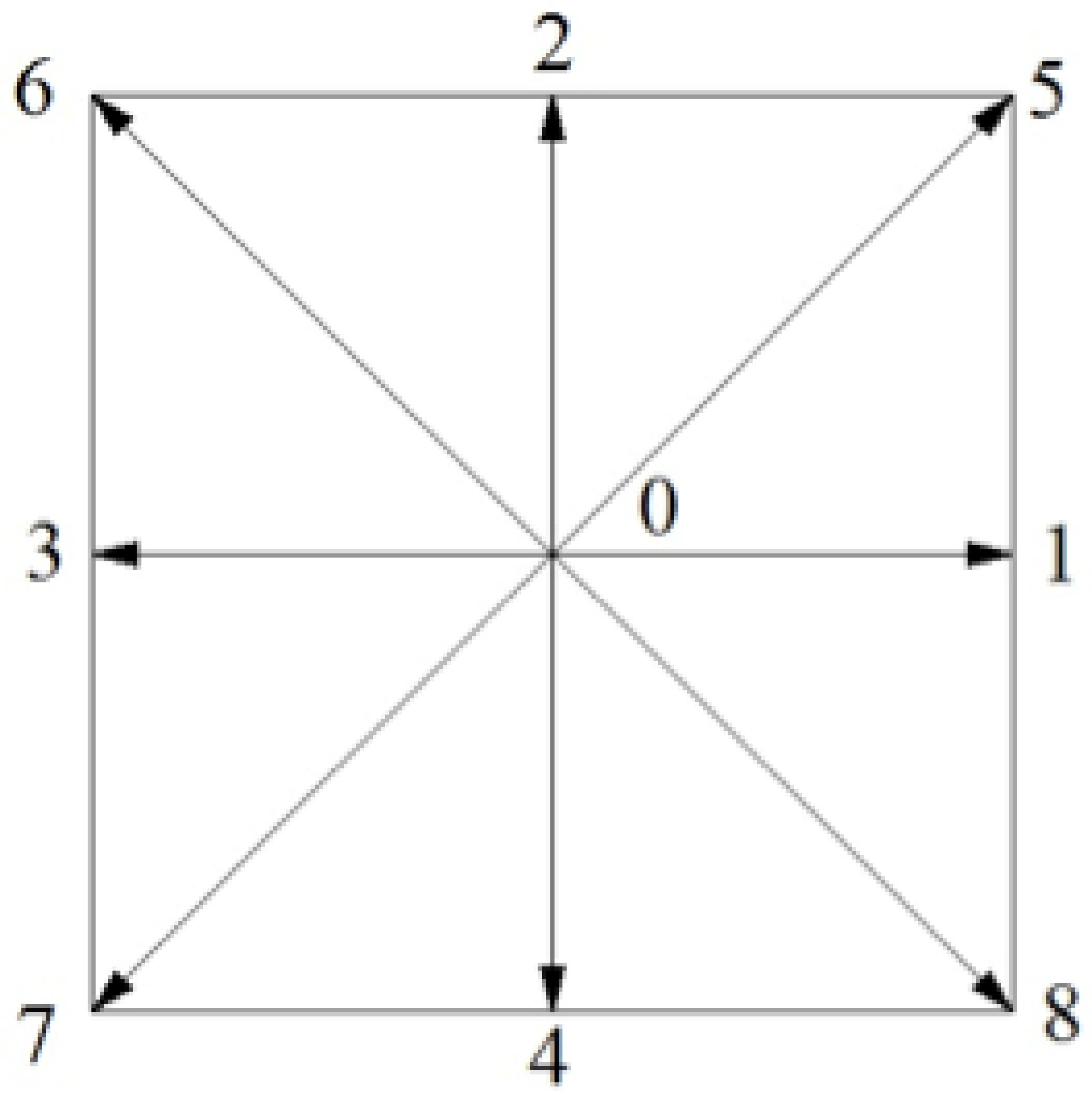
Figure 2.
Discrete lattice velocities of LBGK D2Q7 model [46] and corresponding grid.
Figure 2.
Discrete lattice velocities of LBGK D2Q7 model [46] and corresponding grid.
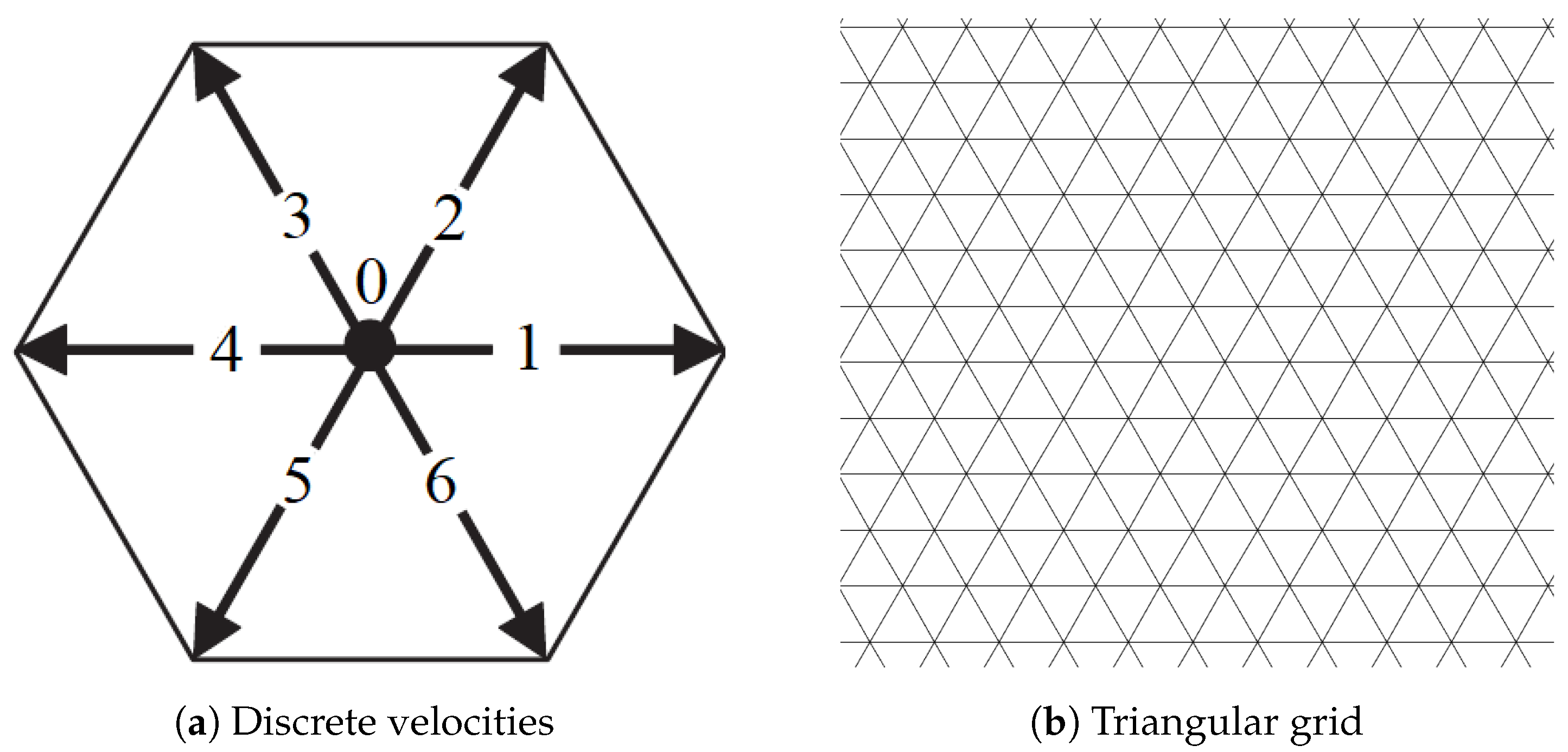
Figure 3.
Discrete lattice velocities of LBGK D2Q9 model and corresponding grid.
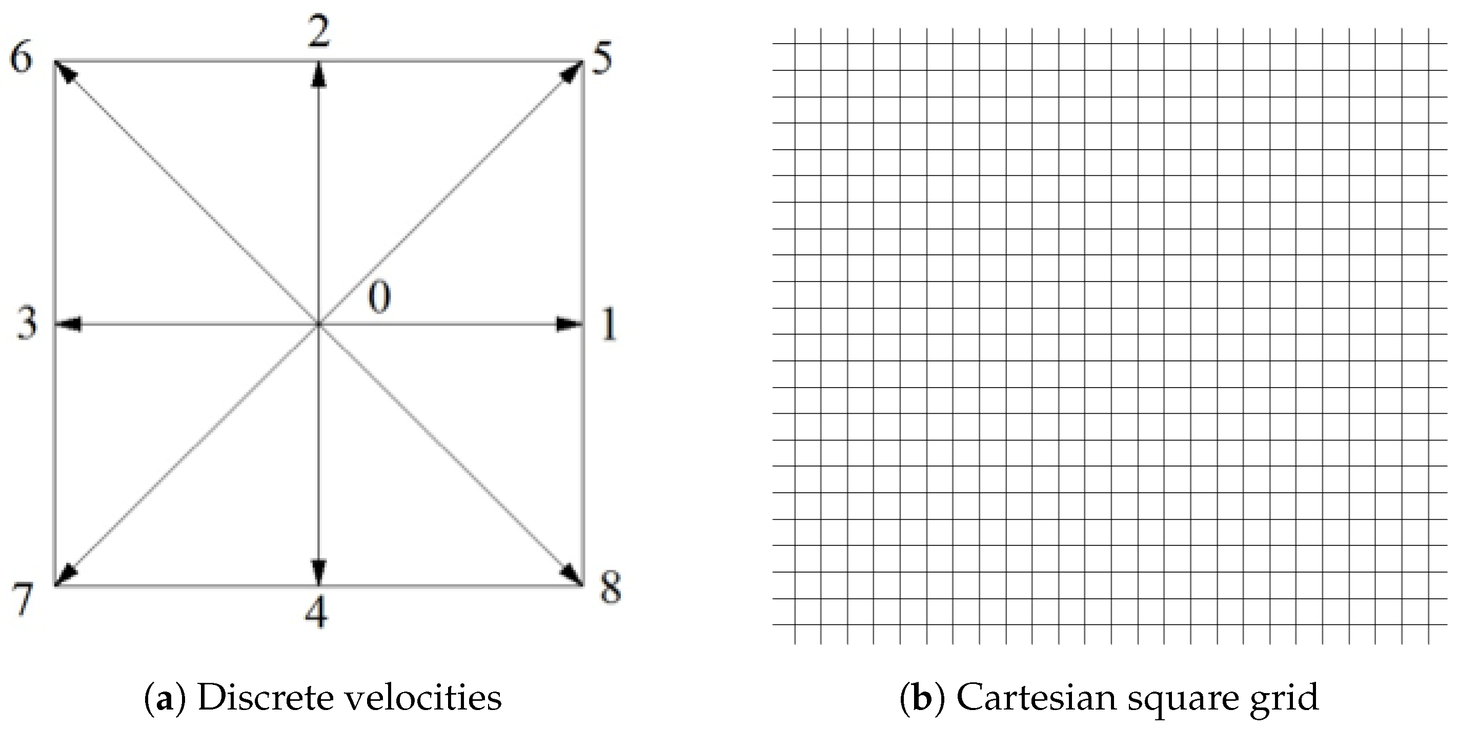
Figure 4.
Body-fitted grid for a circular cylinder.
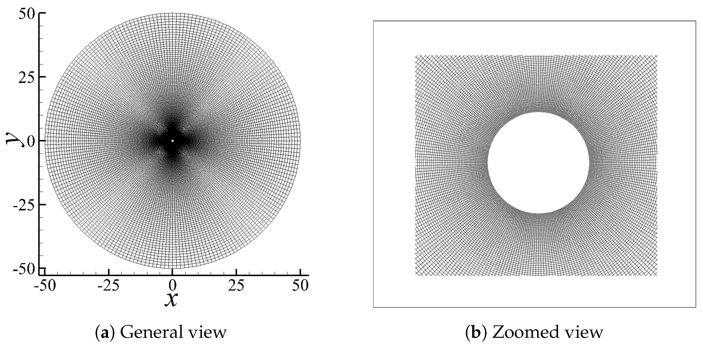
Figure 5.
Coordinate transformation from the physical domain to computational domain.
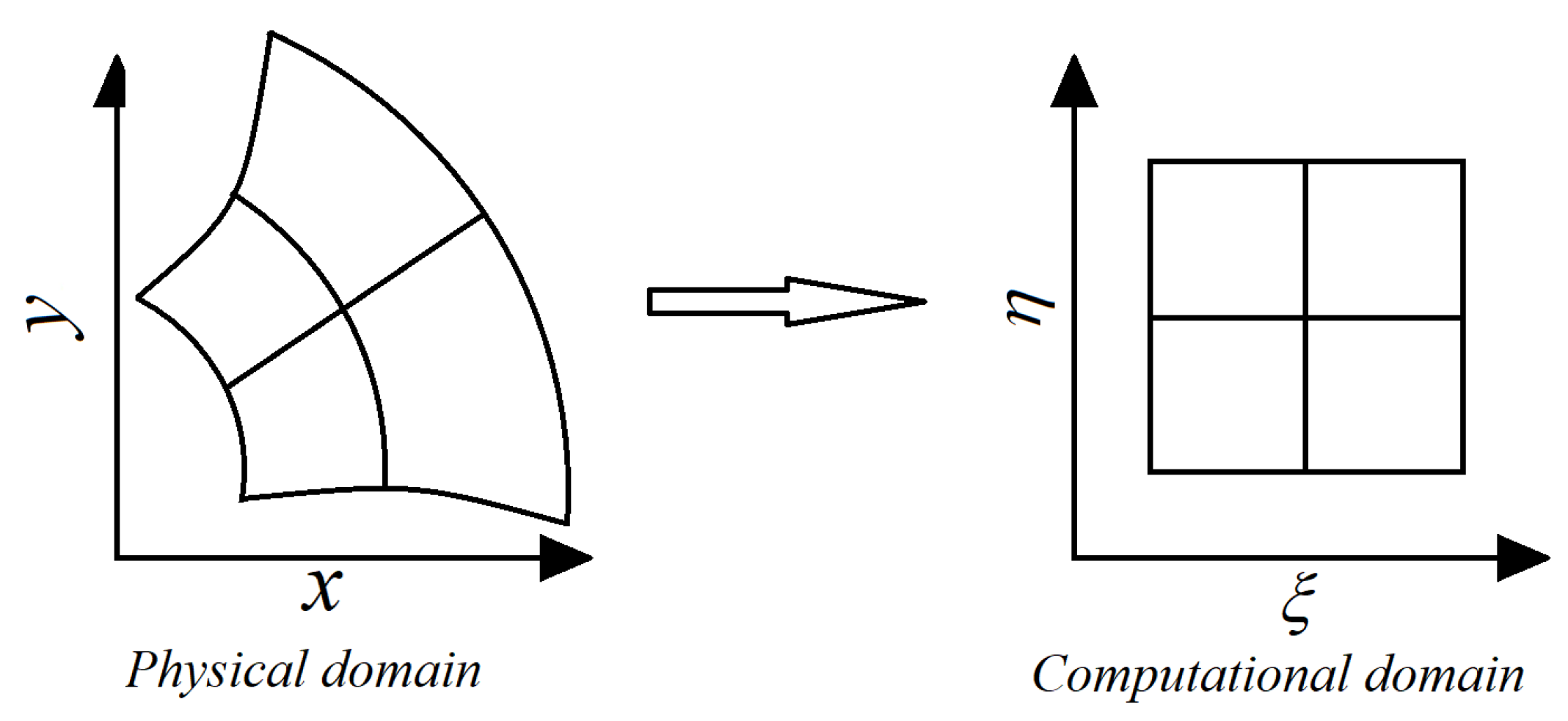
Figure 6.
Streaming process on a computational domain, interpolated and transformation to a physical domain.
Figure 6.
Streaming process on a computational domain, interpolated and transformation to a physical domain.
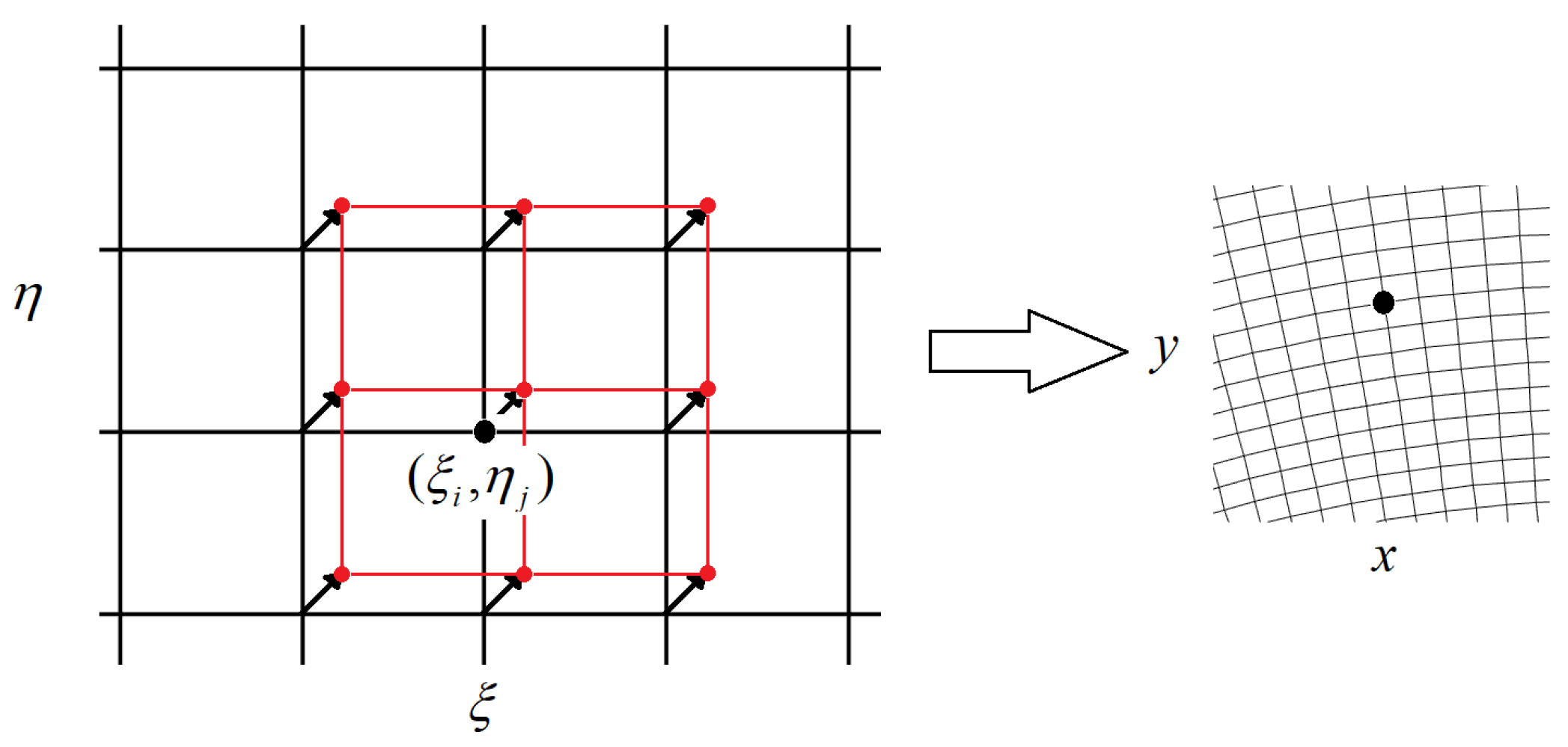
Figure 7.
Streaming of fluid particles in discrete direction [52].
Figure 7.
Streaming of fluid particles in discrete direction [52].
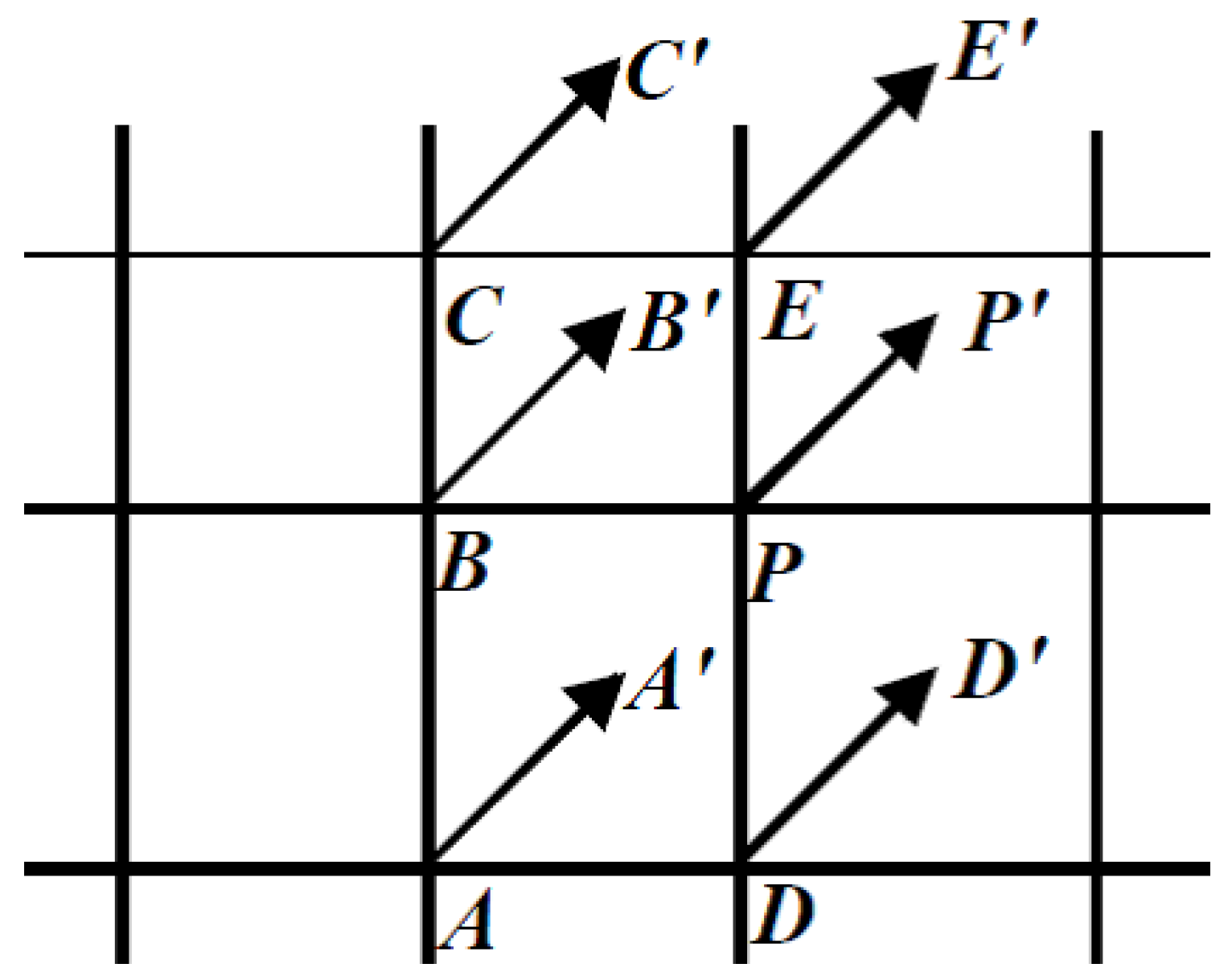
Figure 8.
Grid structure and discrete velocities of rectangular LBM.
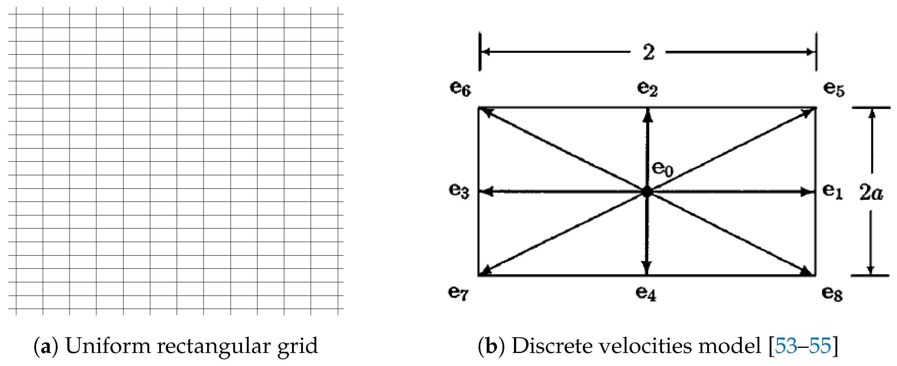
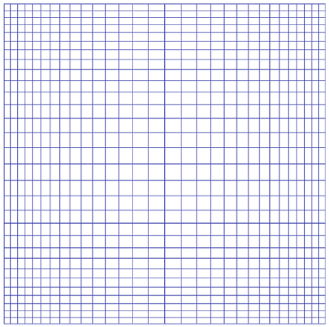
Figure 10.
Streaming demonstration on the non-uniform rectangular grid.
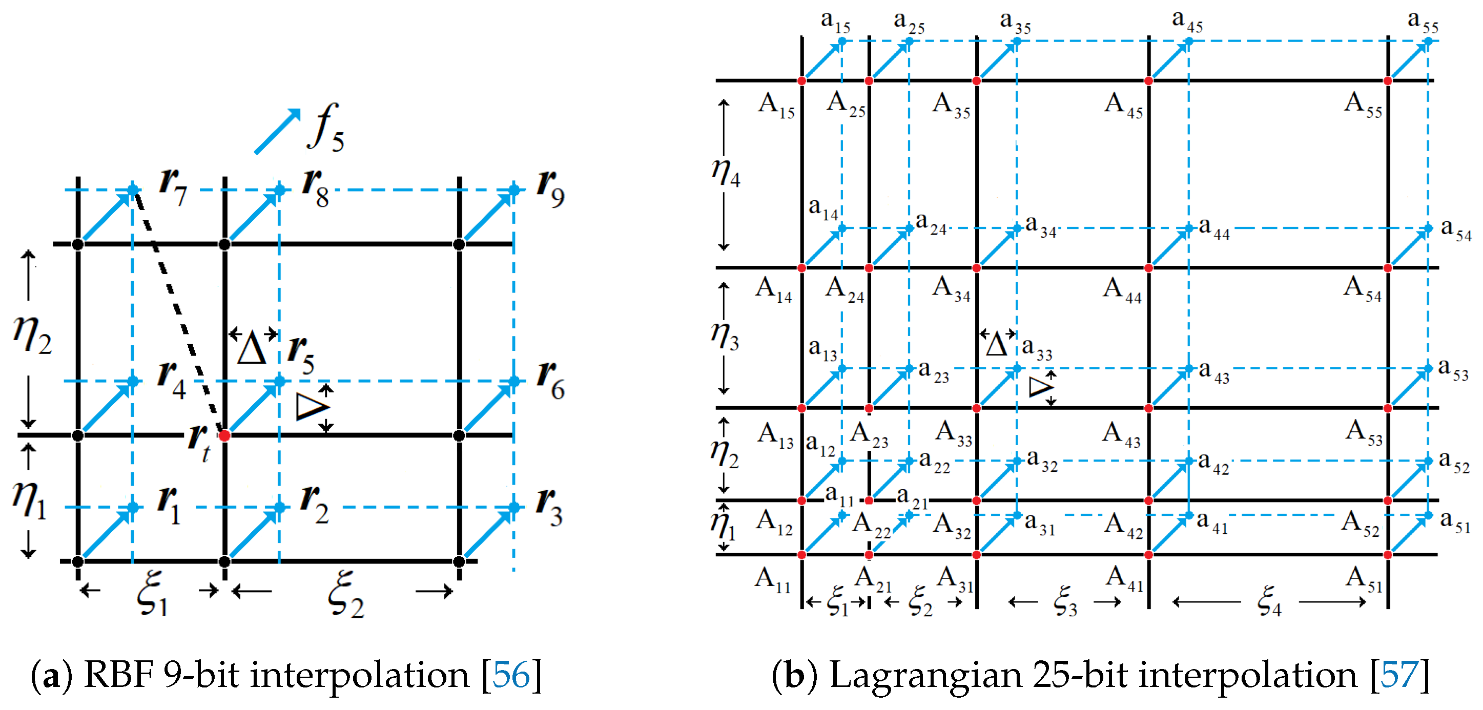
Figure 11.
The computational procedure of V-cycle.
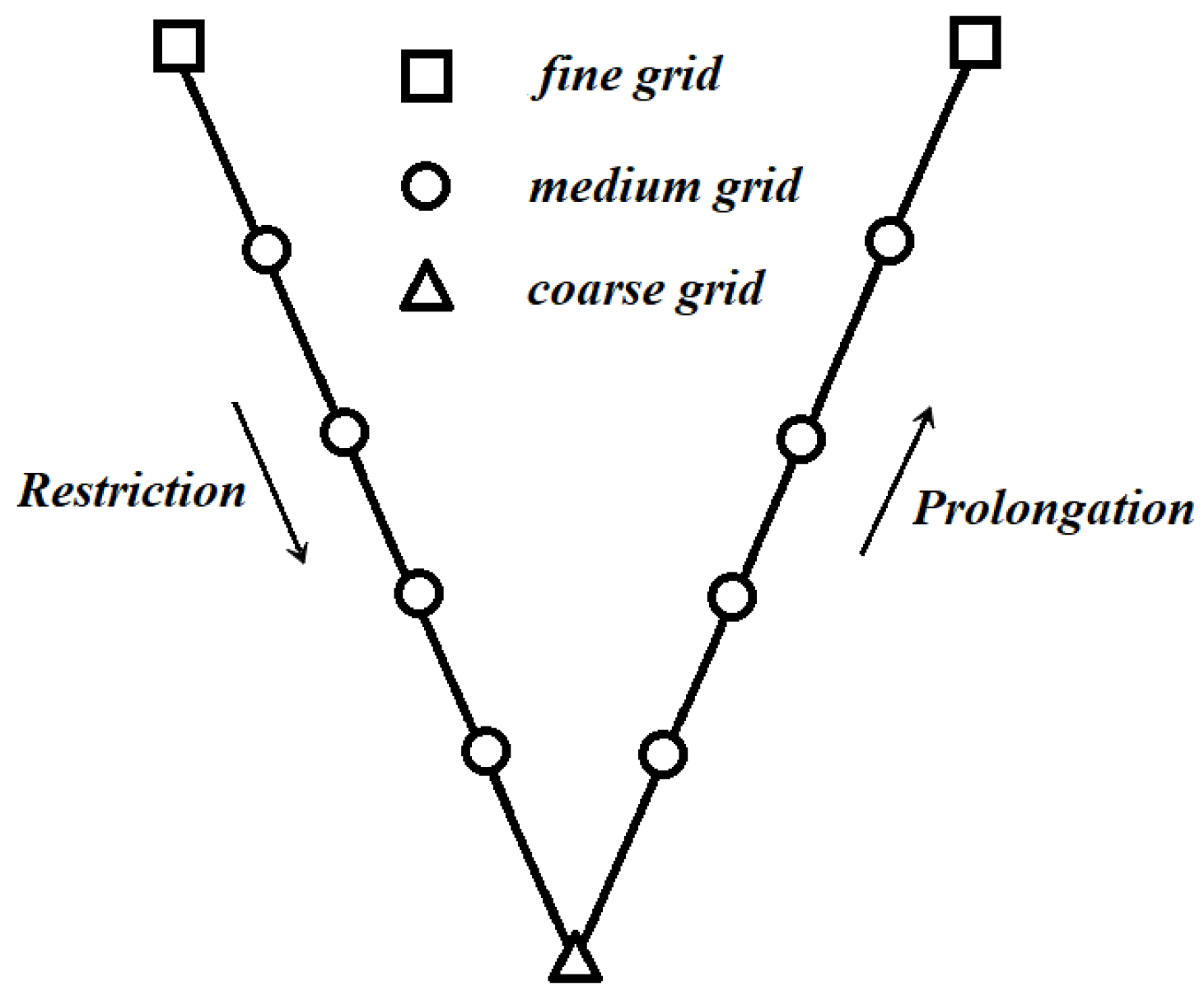
Figure 12.
Numerical diagram for the multigrid V cycle.
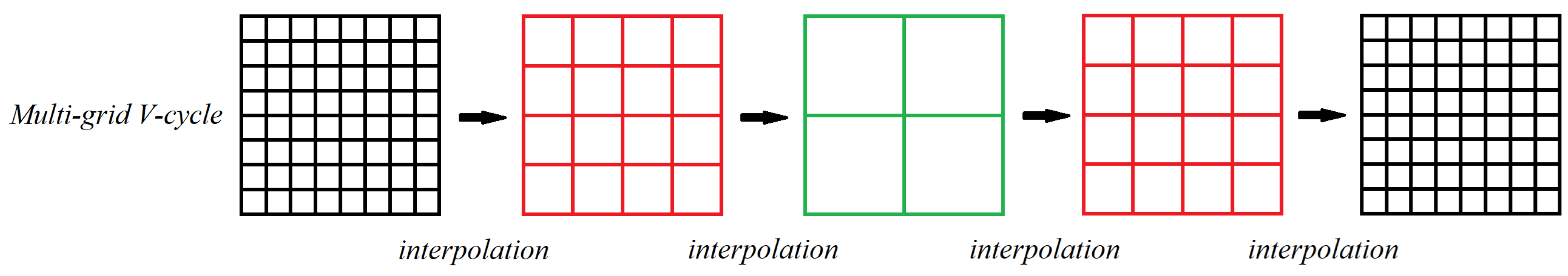
Figure 13.
Non-uniform Cartesian square grid.
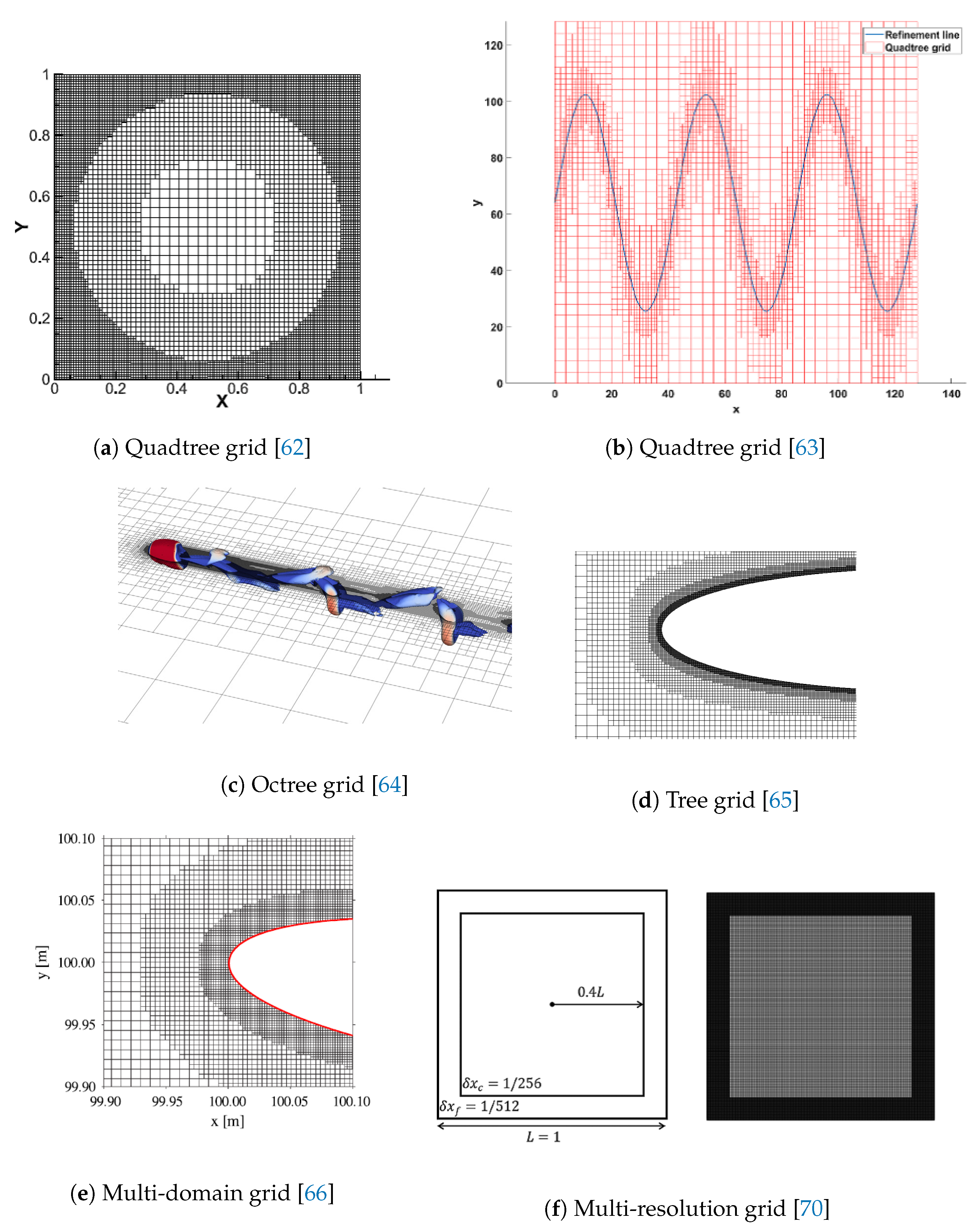
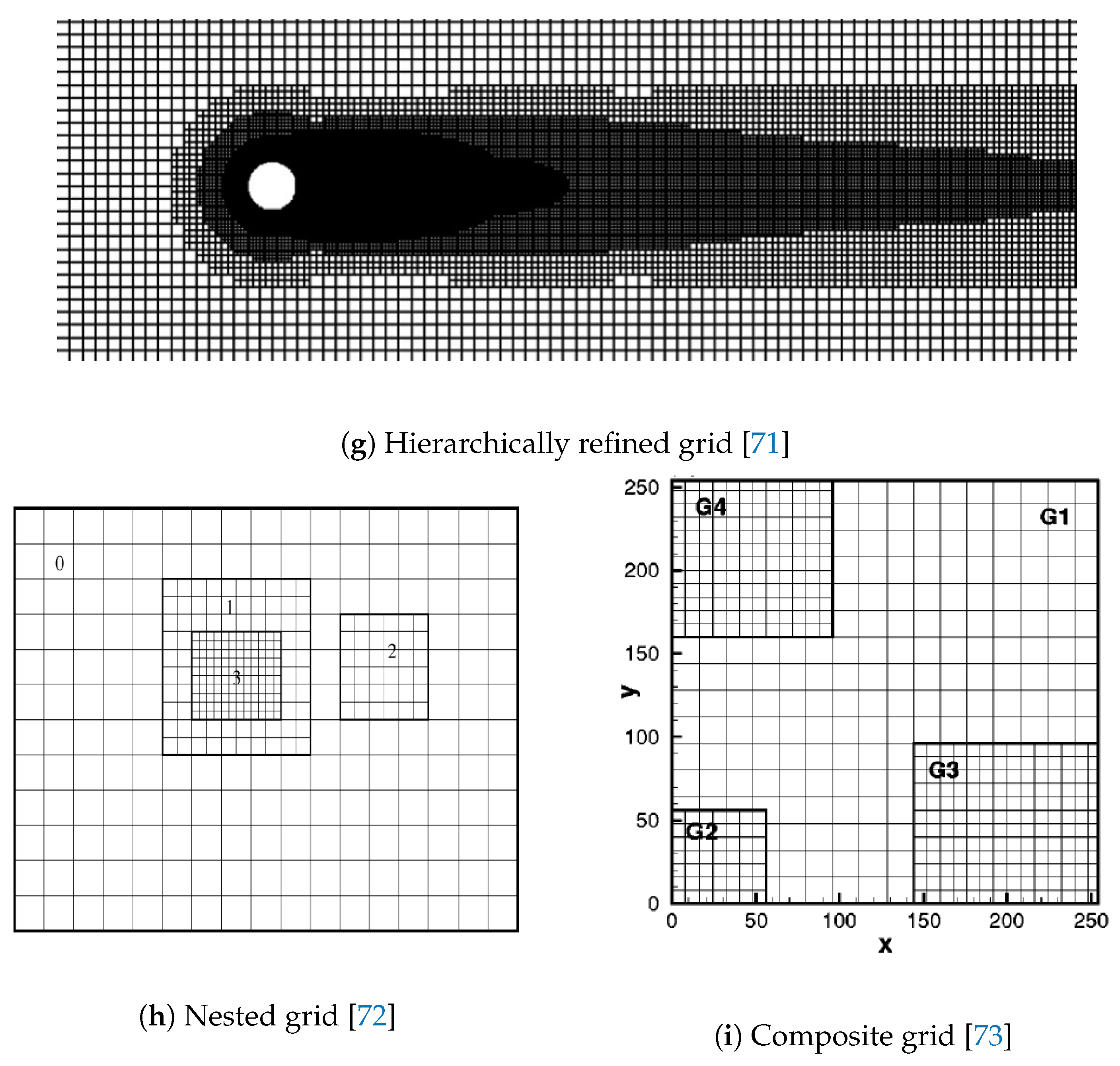
Figure 14.
Serrations on contours on the overlapping borders
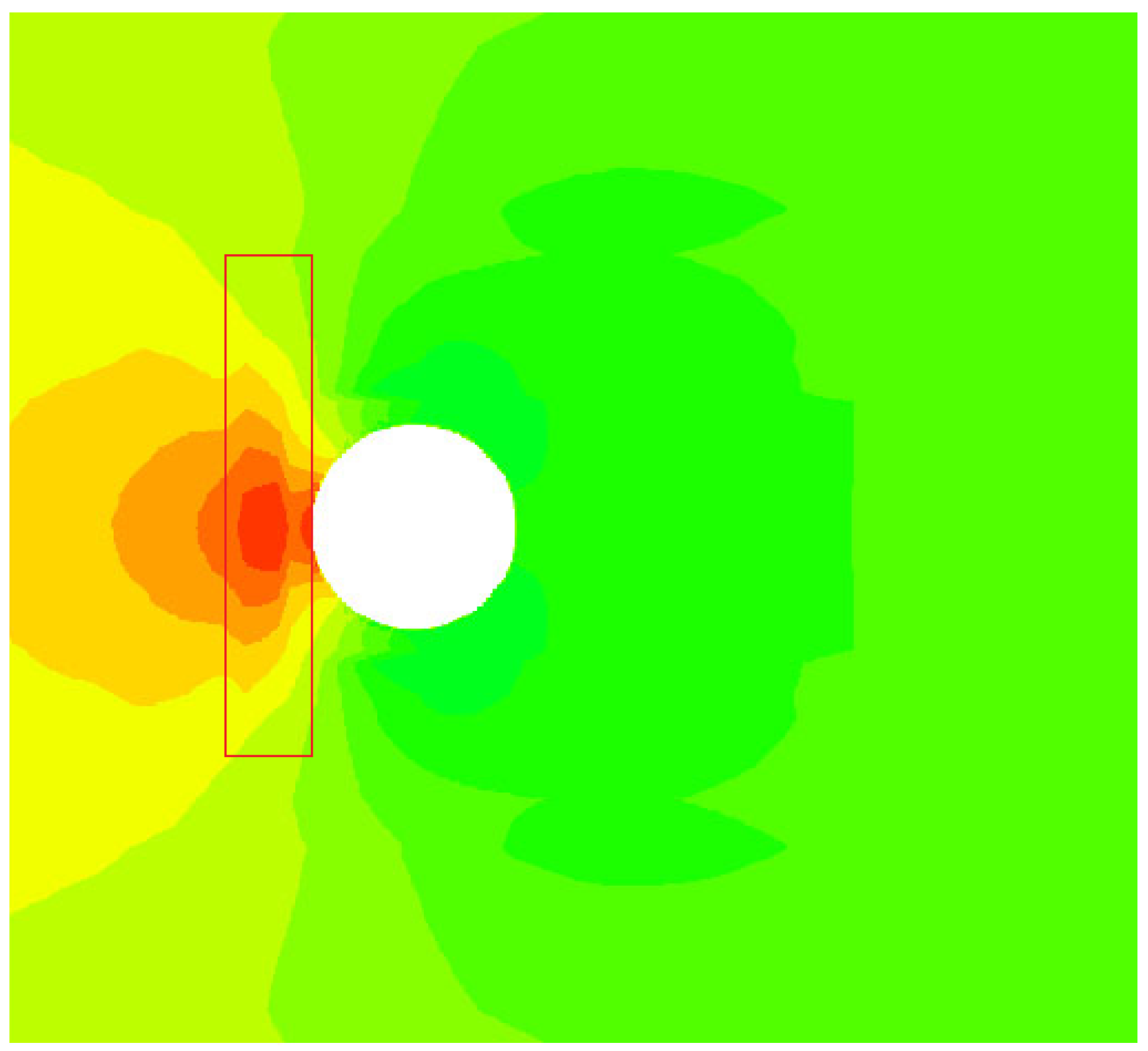
Figure 15.
Unstructured grid
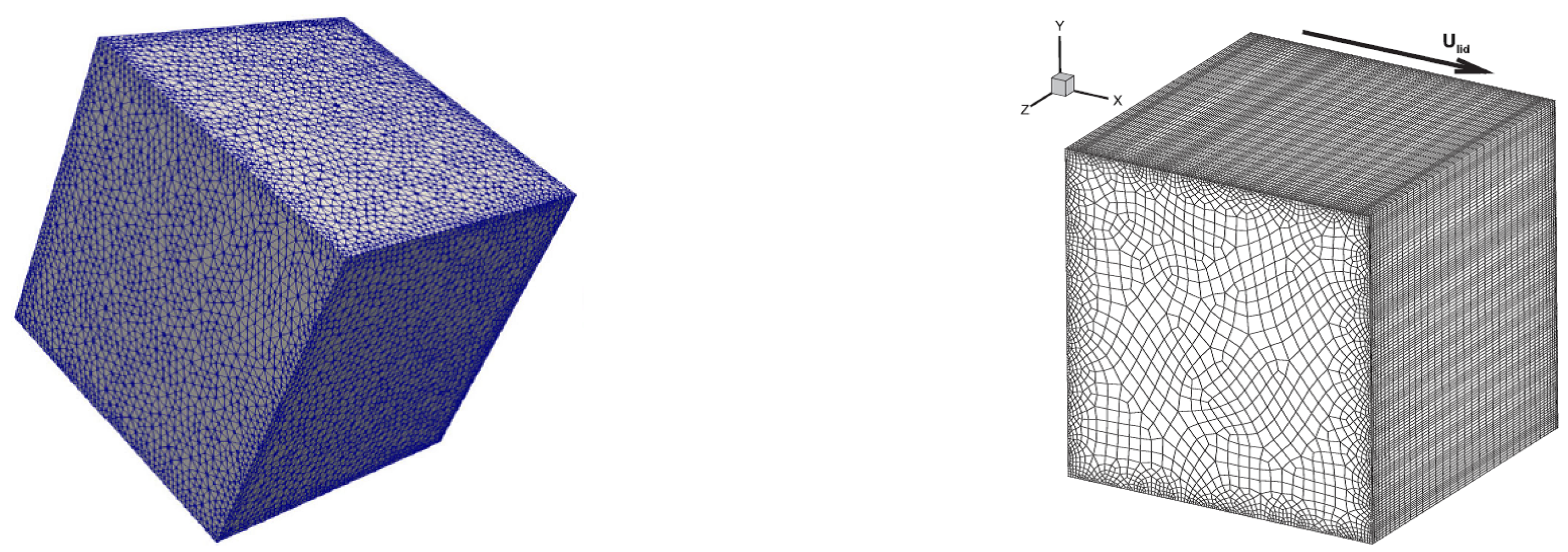
Figure 16.
Diagram of finite elements sharing one node [75].
Figure 16.
Diagram of finite elements sharing one node [75].
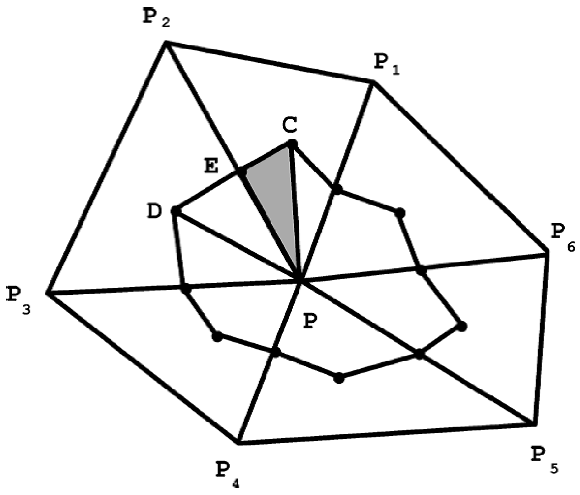
Figure 17.
RBF based interpolation on unstructured grid.
Disclaimer/Publisher’s Note: The statements, opinions and data contained in all publications are solely those of the individual author(s) and contributor(s) and not of MDPI and/or the editor(s). MDPI and/or the editor(s) disclaim responsibility for any injury to people or property resulting from any ideas, methods, instructions or products referred to in the content. |
© 2025 by the authors. Licensee MDPI, Basel, Switzerland. This article is an open access article distributed under the terms and conditions of the Creative Commons Attribution (CC BY) license (http://creativecommons.org/licenses/by/4.0/).
Copyright: This open access article is published under a Creative Commons CC BY 4.0 license, which permit the free download, distribution, and reuse, provided that the author and preprint are cited in any reuse.


