
Submitted:
30 April 2023
Posted:
01 May 2023
You are already at the latest version
Abstract
Grid refinement is used to save computing costs while preserving high precision of fluid simulation. In the Lattice Boltzmann Method, grid refinement often uses interpolated values. We found a method, where interpolation in space and time is not required. For this purpose, we used the moment matching condition and rescaling the non-equilibrium part of populations, and developed the recalibration procedure that allows to transfer information between different LBM stencils in the simulation domain. Then, we build non-uniform lattice which uses stencils with different shapes on the transition. The resulting procedure is verified on the 2D Poisselle flow and the advected vortex benchmark. In prospect, grids with adaptive geometry can be built with the use of the proposed method.
Keywords:
Lattice Boltzmann Method
; Grid refinement
; non-uniform grid
; moment matching
1. Introduction
Lattice Boltzmann Method (LBM) is one of the state of the art methods for computational fluid dynamics. It is a curious case of how the cellular automata application [1] had evolved to model fluids, and subsequently was proven to be a rigorous numerical scheme for integrating the kinetic Boltzmann equation with the use of Gauss cubatures [2]. From the lattice gas stage of the evolution of the method, it inherited the use of rectangular meshes, which are more common in LBM simulations rather than in other hydrodynamic schemes, such as finite element and discontinuous Galerkin methods [3].
Compared to other methods in computational fluid dynamics (CFD), LBM stands out as a lightweight, efficient method with high locality and many options for parallelism [4,5]. The downside is the limited fluid parameter range where LBM, in its classical formulation, works. It is known to lack Galilean invariance, be working in the range of low Mach numbers, and for isothermal flows. Even in that range, many applications are found, such as mesoscale modeling in additive manufacturing [6]. Moreover, with high popularity of the method, many advanced variations were developed for compressible flows, thermal flows and additional physics, and LBM is used in almost every area of CFD.
In this work, we study the adaptive meshes for LBM. In a simulation of a model with several characteristic scales, where both large-scale background flow and small-scale flow variations have to be reproduced, one can use finer mesh for the areas where it is required, and save the computational cost by coarsening the mesh in the area with lower gradients of fluid properties. Adaptive meshes are also used to cover the areas with fine geometry features, such as thin channels. In the flow around the geometry with high curvature, or flat boundary that is not parallel to the Cartesian axes, the rectangular mesh has to be either sufficiently fine to resolve it, or replaced by a mesh that is conformal with the fluid-solid boundaries in the model. Since the classical LBM is constructed for rectangular meshes with a mesh step and time step equal to unity in non-dimensional units, in all these cases, there is an issue of information transfer between different mesh resolutions, different mesh geometries, and an issue of writing LBM for non-rectangular mesh.
Over the years, many researchers have solved the issues by supplementing LBM with some other numerical method. When mesh is refined in some regions, the information is transferred by interpolation in space and/or time. There are two ways of refining the lattice: node-based and cell-based [7,8]. In a node-based approach, a node is added in between each pair of cells. In a cell-based approach, a lattice node is interpreted as a cubic cell, and each cell is subdivided into smaller cubes.
In the node-based methods [7,9,10,11], the order of interpolation can be increased by using more nodes in the reconstruction of the populations [11,12], or by the use of the information on fluid moments to increase the accuracy of the relevant quantities only [13].
Cell-based methods [8,14] have the mass-conserving property. However, in the conventional method [8], the information transfer from coarse to fine mesh, which is often referred to as ’explode’, is, essentially, an interpolation with a polynomial of the order zero: the values are just copied to the nearest cells. An extension with improved accuracy was proposed [7,14]. The mass-conserving method is used in software like PARAMESH [15], waLBerla [16].
There are other methods to modify LBM so as to work with non-uniform meshes, such as finite difference LBM [17,18,19], finite volume and finite element methods [20,21,22,23,24] which can adapt LBM to curvilinear, tetrahedral and unstructured mesh geometries, Taylor series expansion and least-squares methods [25].
Since in the areas with high space resolution finer time step is desired as well, interpolation in time is also used, however, it can be avoided [26,27].
The motivation of the current study is based on the following observation. As a numerical scheme for the kinetic Boltzmann equation, LBM uses a set of discrete velocities to compute moments of the particle distribution function with Gauss quadrature rules. Various sets can be chosen as long as there are enough points in the quadrature to integrate polynomials of a given order [28]. The discretization of the Boltzmann equation in space-time is performed by integration in the direction of the characteristic [29]. The integration along the characteristic is first order, but, with a change of variables, the second order scheme is obtained. The velocity sets are chosen to form a uniform lattice in space, so that the streaming in the direction of the characteristic moves the particle from one lattice node to another.
What if we choose an arbitrary lattice, that fits the spatial and temporal scales and the geometry of our model, and choose a velocity set for each node in a way that every node is connected to its neighbors? If it is possible, than no other scheme except for the basic LBM is introduced in the model, interpolation is avoided, and the order of accuracy depends only on the proper LBM construction.
Methods, where LBM adapts to a stretched [30] or non-rectangular [31] mesh exist. The fact that a composition of different stencil was not used for adaptive grids before is due to the following issue. A lattice with varied geometry requires different discrete velocity sets in some nodes, and a discrete particle distribution function corresponds to each velocity. These discrete particle distribution functions are the populations that are updated in the LBM. We come to a situation where, in general, there are nodes in which the numerical scheme is constructed differently and operates on a different number of populations, and it is not known how these population sets can be converted into one another.
A well-known method of rescaling was used in the original grid refinement method [9], and improved in further works [32]. This was motivated by the change in the value of the time step, which required change in the collision parameter that controls the viscosity, and, in turn, the non-equilibrium part of the distribution functions. The change in the quadrature rule requires further transformation.
Our solution for the issue is motivated by a success in another area of advanced LBM variations. In [33], a revolutionary method of variable rescaling was introduced for modeling high-Mach flows. Even with classical LBM collision operators and no other modifications, flows with Mach numbers over were reproduced. The work had put a start for many new development for complex flow simulations. The scheme was extended and applied for various compressible flows [34,35,36,37,38,39] Recalibrating the populations to the flow velocity temperature for the collision step is known to improve stability [40]
Here we propose to use this method of rescaling for construction of non-uniform grids. Based on the moment matching condition from [33], we develop a population recalibration method that allows to perform streaming between LBM nodes in which the numerical parameters used in construction of LBM method (time and spatial scales, and the velocity set) are different. In general, we identify the numerical parameters that are used to discretize the Boltzmann equations, and find a method to convert a set of LBM populations from a LBM node to an LBM node where LBM was constructed with different parameters.
In the following text, in Section 2, we remind the construction of the LBM method, and what is required to recalibrate LBM variables from one set to another; in Section 3, we propose an algorithm for LBM simulation on a non-uniform grid with the use of the proposed recalibration; in Section 4, we evaluate the resulting method on the trial problems, in Section 5, we discuss the impact of the results.
2. Theoretical Background
2.1. Lattice Boltzmann Method and its Parameters
The kinetic Boltzmann equation is
where — is a single particle distribution function, and its arguments are time, spatial coordinate and particle velocity, and is the collision term.
Macroscopic flow parameters (density , flow speed , and temperature ) are the moments of :
where D — is the number of spatial dimensions.
In LBM, the integration in (2) is performed numerically. Taking into account the solution (3), the integration kernel is
Let us take a quadrature rule with the order of accuracy equal to n
where , are the quadrature points, and are the corresponding weights. The expression is exact when is a polynomial of the order no higher than n.
Other moments are obtained in a similar fashion:
The equilibrium discrete populations are
The standard polynomial representation of [29] can be obtained by expanding this expression in the Taylor series:
By inserting (10) and in (6), (8) the moments are obtained exactly if the chosen quadrature rule is at least of the fourth order of accuracy.
In this derivation, has been introduced as a scheme parameter in (4). It allows to scale , therefore, it provides a connection between time and space scales and controls the lattice geometry. Taking the expression for into account, it is also associated with the model temperature and the speed of sound. In the current work, athermal LBM is considered, and remains a numerical parameter in the scheme construction. For athermal LBM, the 5-th order quadrature is enough [28].
In this work, the collision operator is taken in the Bhatnagar-Gross-Krook (BGK) form [41,42]:
where is the collision parameter that controls the relaxation rate of populations and the fluid viscosity.
Let us take a uniform lattice with mesh step . Then, (11) is discretized on a time step in two successive steps:
In (13), should point from one node to another, therefore, every velocity in the set should be scaled accordingly. The parameter is used to scale . For example, the widely used D2Q9 set, which is
corresponds to .
Thus, according to (13), (14), LBM method consists of the two steps: streaming from one node to another in the direction of , and a local collision operation.
Let us define the LBM stencil as a complete set of scheme parameters that uniquely define LBM streaming: quadrature points and weights, scaling coefficient , time step . We denote the stencil by inserting these parameters in the brackets, i.e. . The common D2Q9 LBM stencil (15) with is denoted as hereafter.
The fluid viscosity is derived with the Chapman-Enskog analysis as [29]:
Finally, given a lattice and a fluid with viscosity equal to , to use classical athermal LBM with BGK collision, we have to ensure that each vector points exactly from one lattice node to another, the quadrature set is enough to integrate with the 5th order of accuracy, and (16) is satisfied.
2.2. Recalibration of Populations
In LBM with adaptive grids, lattice nodes may have varying stencils. For the information exchange between LBM nodes that operate with different LBM stencils, we need to know how the population sets are converted into one another. To construct the method of recalibration of populations from one stencil to another, let us find out what changes are required with the change of , , and the set of quadrature points.
Let us remark that we allow the stencil, and, thus, , vary in time and space, and the derivation of (11) requires inserting under the derivative [43]. There is no contradiction here. In each node, we construct LBM as if it is on a uniform grid. In the following, we find out how the information is converted between LBM constructed for different stencils.
2.2.1. Recalibration with
In other words, the populations are collided in and travel to .
To find the relationship between population which travel from the node according to different stencils, let us use Chapman-Enskog analysis. Taking into account only the term that is linear in the Knudsen number ,
and
Let us consider conversion between stencils with differ only in : D2QM() and D2QM(). Let us take a coarse stencil with time step and relaxation parameter , and a fine stencil with and . By inserting (19) into (17) we get
and a similar relation for the fine stencil. By equating in the expression for the fine and the coarse stencils, we get a well-known relationship [9]
and the relationship between and is obtained be requiring the invariance of fluid viscosity (16) .
2.2.2. Recalibration with both and
Let us take two stencils DNQM and DNQM which correspond to the same quadrature , but different , , . We have
and, instead of (22),
Let us find how depends on the stencil. Let us express it through the derivatives of the physical quantities , . From (10) and (19), we get
Time derivatives in (26) are replaced by the space derivatives with the use of the conservation laws
where
The time derivative is expanded,
2.2.3. Recalibration with a change in quadrature
Let us construct the conversion between populations in D2Q and in D2Q.
The conversions in (21), (32) are between the stencils of the same quadrature , but different . Therefore, these are the conversions between LBMs with different collision operators, which are essentially different LBM equations, and the conversions are giving the correct non-equilibrium part of the populations.
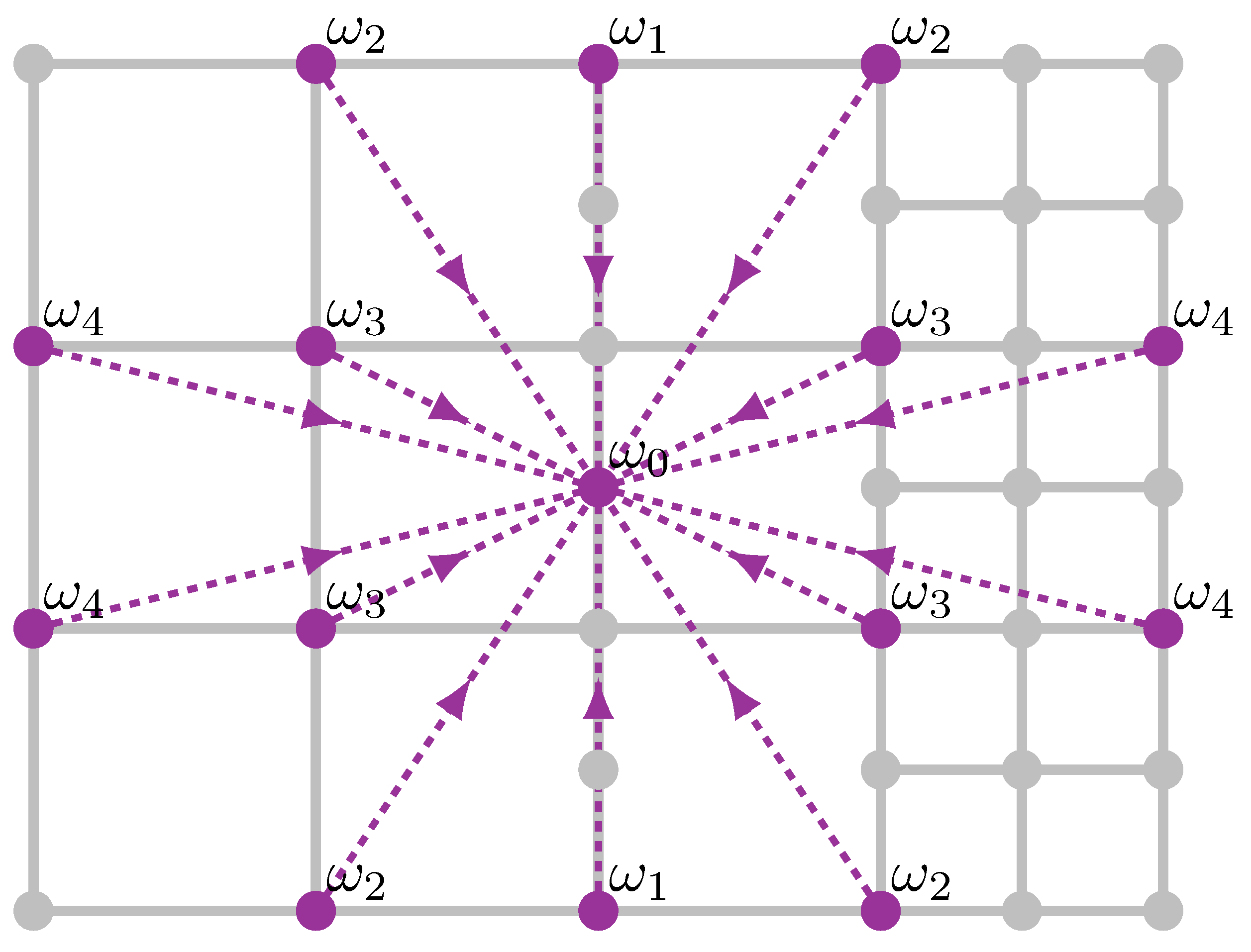
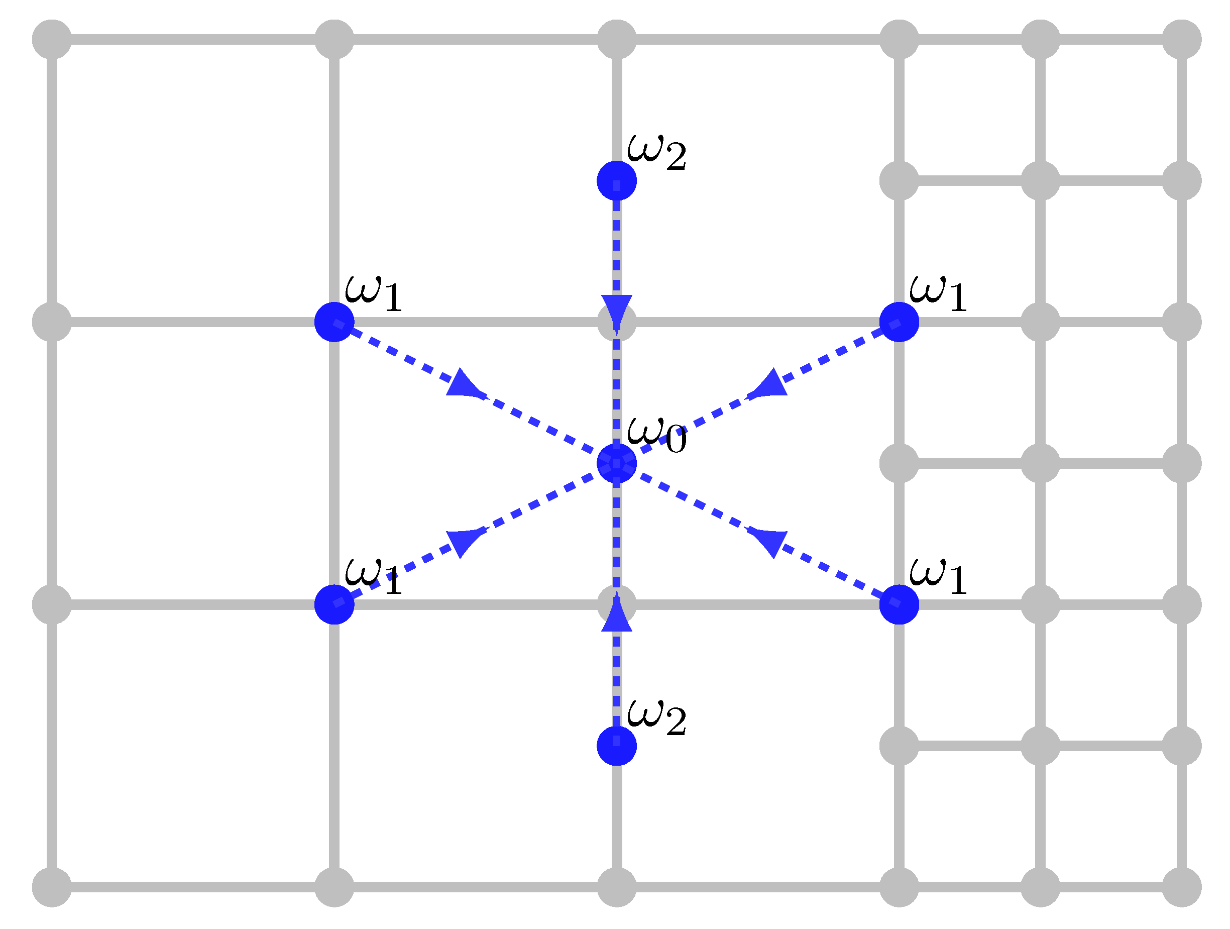
When the parameter remains the same, the moment matching condition [33,34,35,36] is used for conversion. It is required that the change in the LBM populations does not lead to the change in the physical moments:
The number of equations in the linear system (33) depends on the order of approximation of the quadrature and its symmetries [28,29,44]. For athermal fluid physics, we require at least
Additionally, an explicit relationship can be found for (which corresponds to the zero discrete velocity vector) with (7):
Similar relationship can be written whenever stencils have a share discrete velocity.
Relations (33), (35) are a system of linear equations, that has to be solved to find the populations of one stencil, while the populations of another stencil are known. In general, the system can be underdetermined or inconsistent. For example, in the conversion from D2Q9 to D2Q15 we have to find 15 unknown populations from computable moments. In this case, we append the systems by equating relationships from (33) to the equilibrium moments [45].
2.2.4. Recalibration with the change of stencil
In total, in the recalibration of populations from D2Q to D2Q two conversions are applied.
First, the quadrature rule is fixed, and , , are modified with (24), (32). This converts D2Q to D2Q. Second, the quadrature is changed with fixed , , and the stencil is converted to D2Q. The two steps can be performed in any order. In any case, in the middle of the conversion, there is a virtual LBM stencil (here, D2Q) for which neither streaming nor collision takes place.
3. Grid Refinement Interface without Interpolation
3.1. Grid Geometry
The recalibration method allows to construct a transition between grids with different time and space steps, if only we construct the stencils that point to/from the lattice points exactly in the uneven grid transition region.
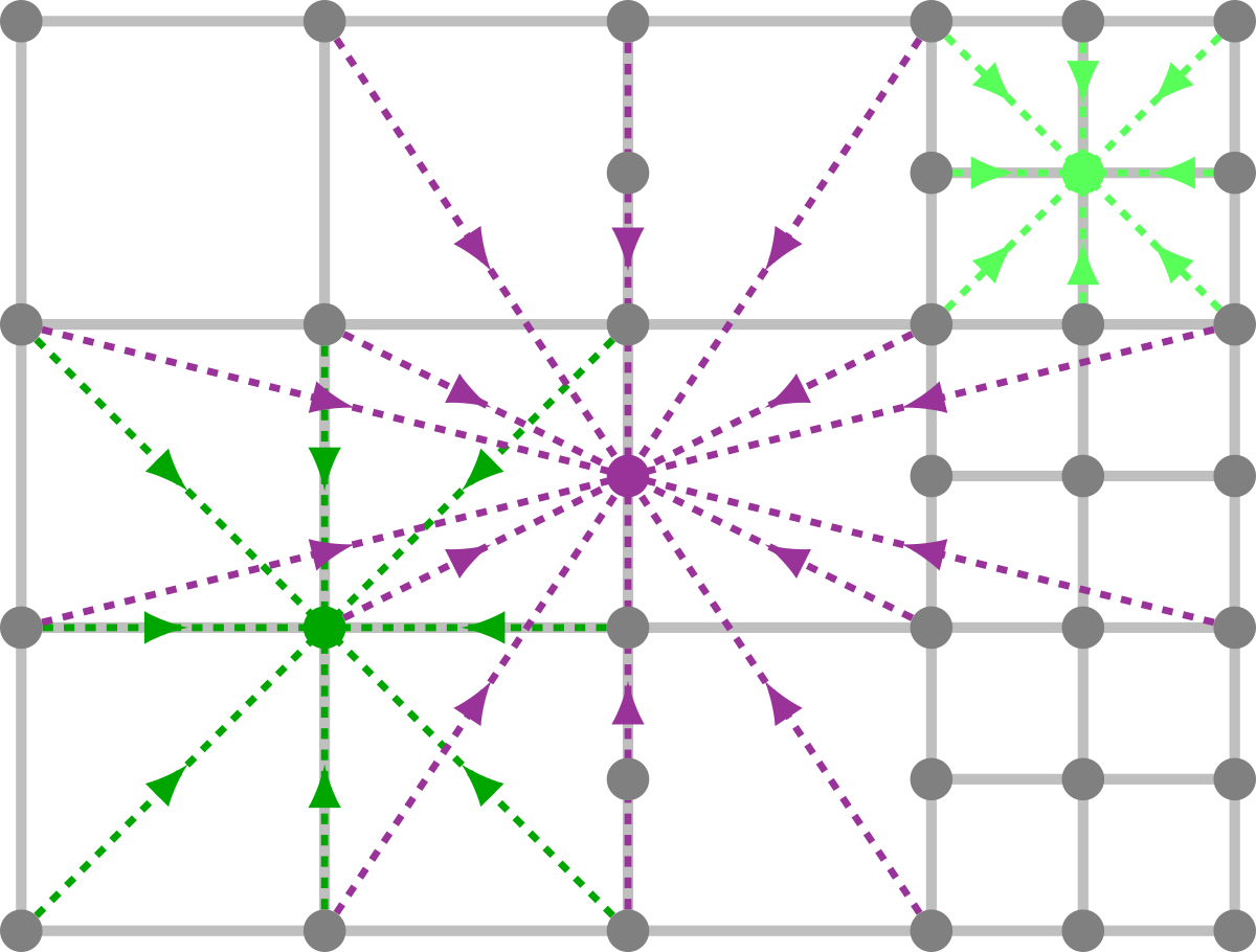
Let us take a grid refinement boundary with coarse uniform grid () on the left side and fine uniform grid () on the right side (Figure 1).
LBM stencils can be used in the ’Pull’ or ’Push’ paradigm, which is relevant for the conversion purposes. In the ’Push’ method, the populations are streamed from a node according to the stencil of that node. After the streaming, the populations in any one node may come from different stencils, and there is no full set of populations in some nodes. In the ’Pull’ method, populations are converted into the stencil of the node before they are streamed into that node. The ’Pull’ method is in the original work [33], and is used in the current study. In case of the uniform grids, no stencil conversions are used and the ’Pull’ and ’Push’ methods are equivalent. The difference of rescaling incoming and outgoing populations in refined grids supplemented with interpolation is reported in [32].
3.2. Stencils and Recalibration
Let us construct an LBM algorithm, in which coarse and fine grids use the classical LBM stencil, and the transition between grids do not require interpolated values, that is, all point from one node to another. This is possible by introducing several transitional LBM stencils.
Let us use D2Q9(1, 1/3) (dark-green in Figure 1) and D2Q9(1/2, 1/3) (light-green) for the coarse and the fine grids respectively. This leads to the classical unaltered D2Q9 LBM in the fine and coarse grids away from the boundary.
For the grid transition, the well-known quadrature derivation rules can be used [46]. D2Q15(1, 25/38) (see Appendix A for the derivation) is a stencil of the 5th order which uses the existing nodes, thus, its can reproduce the moments of the equilibrium distribution at least as good as D2Q9 which is used away from the grid transition. We have also tried the D2Q7(1, 1/4) (details in Appendix A). This stencil performs correct integration for less moments, but is more local. The tests with both stencils are reported in Section 4. In Figure 1, D2Q7(1, 1/4) is depicted, but D2Q15(1, 25/38) can be used instead.
To perform grid transition, we use nodes with the D2Q7(1, 1/4) (or D2Q15(1, 25/38)) stencil (blue in Figure 1) on the integer time steps, and the D2Q9(1/2, 4/3) on half-integer time steps (orange nodes in Figure 1). This is just one of the many possibilities that can be constructed on the boundary transition.
Other configurations can be used depending on the requirements of the model.
When the introduced stencils are used in the ’Pull’ paradigm, the streaming operation at a node requests populations from the neighboring nodes. At the node from where the population is requested from, the recalibration in the target stencil takes place. If it is a recalibration between different variations of D2Q9, (24) is used. If any other stencil is involved, the recalibration is performed in two steps according to Section 2.2.4.
Here D2Q9(1, 1/4) and D2Q9(1, 25/38) are the virtual stencils that are used only as an intermediate state in the conversion of populations.
3.3. Full Grid Transition Algorithm
The initial state corresponds to Figure 1(a).
-
Perform streaming on the coarse grid with the use of the stencils
- (a)
- D2Q7(1, 1/4) (or D2Q15(1, 25/38)) for the blue nodes;
- (b)
- D2Q9(1, 1/3) for dark green nodes. Here the incoming populations at the nodes which are exactly on the boundary are saved in a separate temporary buffer to be used in step 5, since the pre-streaming populations are still needed in the next step.
-
Perform streaming on the fine grid (Fig Figure 1(b)) with the use of the stencils
- (a)
- D2Q9(1/2, 1/3) at the light-green nodes;
- (b)
- D2Q9(1/2, 4/3) at the orange nodes.
- Perform collision on the fine grid at the orange and light-green nodes (Fig Figure 1(b)).
- Perform second streaming to the light-green nodes of the fine grid (Fig Figure 1(a)).
- Restore the values of the boundary nodes from the buffer.
- Perform collision on all nodes according to the stencils in Fig Figure 1(a).
4. Benchmarks
The proposed algorithm was implemented in C++ with the use of the Zipped Data Structure for Adaptive Mesh Refinement (ZAMR) [47] library in the Aiwlib [48] package. The library provides convenient tools to work with binary refined grids based on the Z-order curve traversal. It allows to perform operations on all nodes of uneven grids, and to set flags on the nodes where operations differ. With it, we mark different color of nodes in Figure 1 with different flags and implement the described algorithm.
4.1. Poiseuille Flow
The stationary solution of the Navier-Stokes equation
in the , domain with no-slip boundary in x and periodic boundary in y:
subject to the pressure gradient
is
The flow is modeled with the use of the bounce-back boundary conditions in x [29]. The pressure gradient is simulated with an additional term in the flow velocity in the computation of equilibrium distribution [49] for the collision step. The initial state is equilibrium where
The flow evolves to its equilibrium state (41).
In this benchmark, classical LBM with BGK collision and bounce-back boundary has a well-known problem. The effective channel width can depend on the collision parameter [50]. In this benchmark we fix on the fine grid. Then the viscosity is , and the boundary is considered to be at the distance from the boundary nodes [29].
We refine the grid near the no-slip boundaries. The sizes of the grid are
Where r is the parameter that controls the grid resolution. With , half of the grid geometry is in Figure 2.
The fine grid takes approximately a quarter of the domain. In our benchmarks, such grid geometry performed slightly better than if the grid is refined in the half of the simulation region.
To evaluate the order of approximation of the proposed scheme, the numerical error dependency on r is studied. With the change of r with fixed , the effective channel width and velocity maximum increase. Thus, the error is normalized to . Note that in evaluating the norm in case of non-uniform grids, the contribution of nodes is scaled to the effective area of the node to ensure correct numerical representation of the finite integral.
The blue nodes in Fig Figure 2 serve auxiliary purpose in the scheme and are not taken into account in the total error.
The benchmark results are reported in Figure 3, Figure 4. The results are compared to LBM simulation on a uniform fine grid (light green lines).
We observe that the proposed method of grid transition works correctly.
The D2Q7(1, 1/4) stencil performs better in the space time discretization, and gives the result almost as good as a uniform fine grid. However, the stencil does not reproduce high order velocity moments, and suffers from Galilean invariance errors. That is why its performance with grid refinement is more consistent with lower g (Figure 4).
The discretization errors for the D2Q15(1, 25/38) are higher and show the first order of accuracy. The source of the error is yet to be found. The dependencies of this stencil in the space-time grid are the longest of all other stencils in the constructed scheme. The low angle of the space-time characteristics may cause such behavior.
Let us compare the order of accuracy of our algorithm with the already known schemes for constructing non-uniform grids. When using stencil D2Q7(1, 1/4), we get almost the second order of accuracy in each norm, which is more stable than both algorithms with initial-value problem (IVP) and boundary-value problem (BVP) types of interpolation in [26], and similar to cell-vertex and cell-centered with linear explosion hybrid-recursive regularized (HRR) algorithms in [7]. When using stencil D2Q15(1, 25/38), we get the order of accuracy close to unity, which is resemble method with IVP interpolation in [26] and cell-centred with uniform explosion HRR algorithm in [7].
Let us note that the benchmark results can be improved by the use of advanced collision and boundary conditions [29,50]. Here we demonstrate only the impact of the proposed recalibration method, thus, the classical LBM with BGK collision is used.
In Figure 5, the difference between numerical and theoretical solution is plotted vs the x coordinate. Here , , . It can be seen that the grid transition introduced an error an leads to the non-physical current in the x direction, and the error, indeed, appears on the grid boundary, and is not caused by the bounce-back boundary.
4.2. Athermal vortex
In the second benchmark, the dynamics of the advected athermal vortex [51,52] is modelled. The initial conditions are
for the stationary vortex, and a constant is added to to model advection. Here is the amplitude of the vortex rotation, R is the vortex radius, T is the lattice temperature. According to the Navier-Stokes solution, the vortex relaxes to uniform flow, and the relaxation rate is proportional to viscosity. In our benchmarks, we set lower viscosity and study the preservation of the vortex shape under the influence of the grid boundaries.
We take the simulation region size , , the left half of the region is refined. All boundaries are periodic. The vortex is initialized in the left half by setting the equilibrium populations on the fine grid with the flow parameters according to (47). The numerical parameters are , , , , .
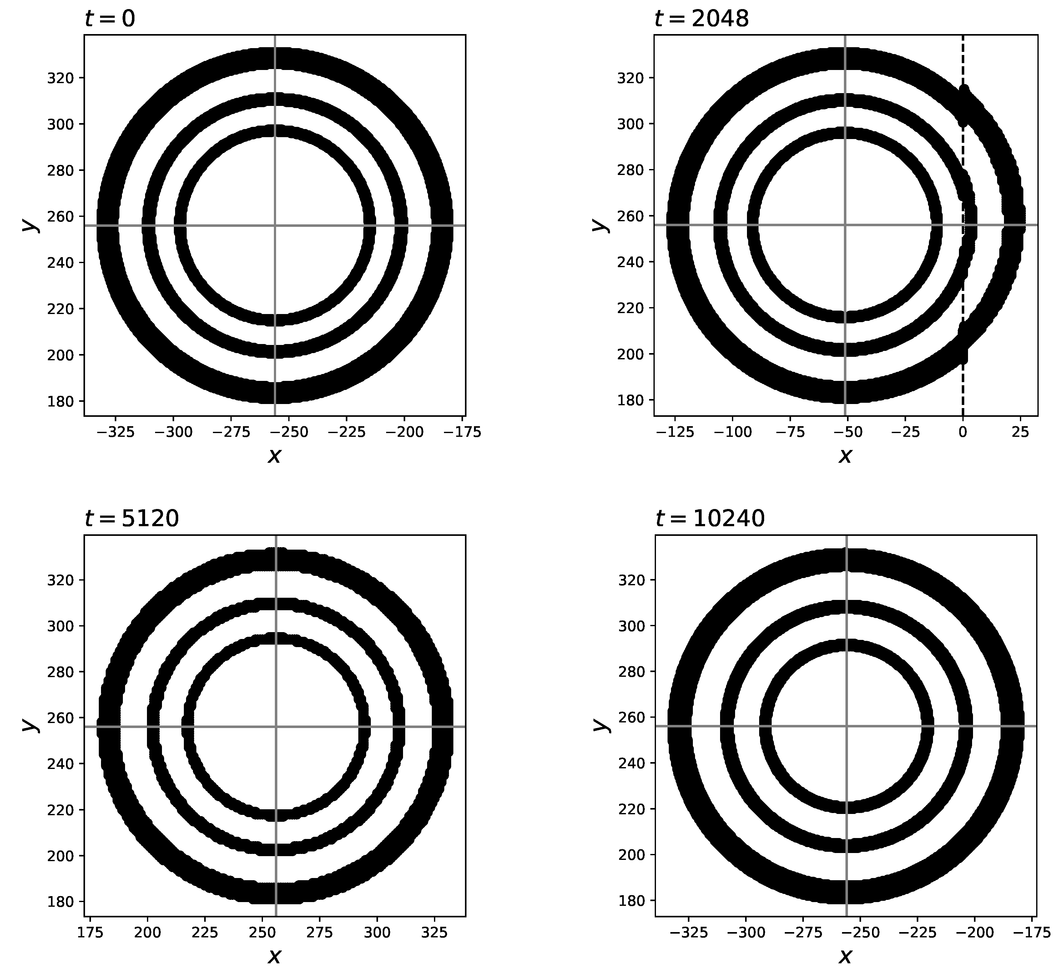
The D2Q15(1, 25/38) stencil is used on the grid transition. Figure 6 shows the moment of vortex interaction with the grid boundary. Its shape is preserved in the interaction, and even after it passes back onto the fine grid (Figure 7). The effect of the transition on the solution can be seen by magnifying the density range on the color map (Figure 6(b)). The effect is several orders below the solution.
5. Conclusion
As a conclusion, we have shown how the moment matching condition [11] can be used to perform conversions between LBM stencils on non-uniform grids. For LBM with BGK collision, we developed the method of recalibration of populations, which extends the one proposed in [9] to variable lattice temperatures, and supplemented it with the method of a transition to a different discrete velocity set.
We proved the recalibration to be valid with 2D benchmarks with one-dimensional grid transition interface. For this purpose, the algorithm that involves intermediate stencils on the transition interface was proposed.
We believe that this is an important contribution because it allows building non-uniform meshes while remaining in the LBM framework, without the use of interpolation, finite differences, series expansion, or other supplementary schemes. The recalibration method is based only on the correctness of quadrature rule in the velocity space, and the Chapman-Enskog analysis. This method can be used for different configuration of mesh interfaces, and even for dynamically refined or moving grids [53].
To apply the method further for more complex grid configurations, a combination of stencils for the grid interface has to be built. After that, the proposed method can be applied to perform the transitions.
The choice of the best configuration is yet to be found. In the following studies, we may search the source of errors that led to worse order of approximation in the Poiseuille flow benchmark.
Furthermore, it is interesting to formulate the recalibration in the ’Push’ framework based on the rescaling of the outgoing populations [32] and moment matching with more than two population sets. By combining a ’Pull’ and ’Push’ types of streaming, a configuration of stencils that lead to a grid transition without the mass loss may be found.
In the work we used the basic BGK collision and the basic bounce-back boundary to focus on the impact of the recalibration method. For other collision operators, the recalibration procedure, and the adaptation of the collision parameter to the stencil, may differ, but may be built on the same principles that were discussed in the current text.
While the classical LBM is known to be limited in the range of its applicability, it is still valid in the vicinity of the equilibrium function with fixed velocity (usually, zero), low Mach number, and on a sufficiently detailed space-time lattice. With the use of the moment matching condition, the LBM can be locally rebuilt with different background flow [33,54,55], with different compressibility assumptions [45]. Thus, the LBM stencil can change both in time and in space to adapt to the flow conditions. The contribution of our work is the demonstration of the fact that the moment matching can also be used to adapt the stencil to the local geometry, or to an increased Reynolds flows.
Author Contributions
Conceptualization, funding acquisition, writing—review and editing A.P.; methodology, validation, formal analysis, investigation, benchmarks, visualization, writing—original draft preparation, A.B.; software, A.I.; supervision, V.L.
Funding
This research was funded by Russian Science Foundation grant number # 18-71-10004
Institutional Review Board Statement
Not applicable
Data Availability Statement
Data can be provided by the authors upon request.
Acknowledgments
Conflicts of Interest
The authors declare no conflict of interest.
Abbreviations
The following abbreviations are used in this manuscript:
| LBM | Lattice Boltzmann Method |
| CFD | Computational fluid dynamics |
| BGK | Bhatnagar-Gross-Krook |
| ZAMR | Zipped Data Structure for Adaptive Mesh Refinement |
| IVP | Initial-value problem |
| BVP | Boundary-value problem |
| HRR | Hybrid-recursive regularized |
Appendix A. Stencils for the grid transition
The stencils for the grid transitions are built according the basic Gauss-Hermite quadrature construction rules. For the constructed quadrature rule to be no worse than the classical D2Q9 variant, we require the expression
to be satisfied for all monomials up to the 5th order ().
The quadrature points are chosen in the grid refinement process. Then, the weights are found by solving (A1) for and . The quantities are assumed to satisfy the standard inequalities , .
This amounts to a total of () equations in general. If the quadrature point configuration is symmetrical in x and y, the equations for all odd powers in or are trivially satisfied. A total of six equations remain to be solved. Therefore, at least five independent weights are required in addition to the free parameter ..
As the most local configuration with five independent shells we choose (Figure A1).
Figure A1.
D2Q15(25/38, ) stencil
The equations to be satisfied are
The solution of the system is
and .
In this work, we also use the stencil with points (Figure A2)
For the fifth order of accuracy, the following relationships have to be satisfied
It is impossible to satisfy all of these with just four parameters, so, among the fourth order equations we choose to satisfy only the equation for , while the equations for and are not satisfied. This is the only choice that results in a correct solution for the Poiseuille flow benchmark.
Figure A2.
D2Q7(1/4, ) stencil
When the relationship for is satisfied, the weights are
with . This is the variant used in the current work.
References
- Wolf-Gladrow, D.A. Lattice-gas cellular automata and lattice Boltzmann models: an introduction; Springer, 2004.
- Shan, X.; Yuan, X.F.; Chen, H. Kinetic theory representation of hydrodynamics: a way beyond the Navier–Stokes equation. Journal of Fluid Mechanics 2006, 550, 413–441. [Google Scholar] [CrossRef]
- Cockburn, B.; Shu, C.W. Runge–Kutta discontinuous Galerkin methods for convection-dominated problems. Journal of scientific computing 2001, 16, 173–261. [Google Scholar] [CrossRef]
- Wittmann, M.; Haag, V.; Zeiser, T.; Köstler, H.; Wellein, G. Lattice Boltzmann benchmark kernels as a testbed for performance analysis. Computers & Fluids 2018, 172, 582–592. [Google Scholar]
- Perepelkina, A.; others. Heterogeneous LBM Simulation Code with LRnLA Algorithms. Communications in Computational Physics 2023, 33, 214–244. [Google Scholar] [CrossRef]
- Zakirov, A.; Belousov, S.; Bogdanova, M.; Korneev, B.; Stepanov, A.; Perepelkina, A.; Levchenko, V.; Meshkov, A.; Potapkin, B. Predictive modeling of laser and electron beam powder bed fusion additive manufacturing of metals at the mesoscale. Additive Manufacturing 2020, 35, 101236. [Google Scholar] [CrossRef]
- Schukmann, A.; Schneider, A.; Haas, V.; Böhle, M. Analysis of Hierarchical Grid Refinement Techniques for the Lattice Boltzmann Method by Numerical Experiments. Fluids 2023, 8, 103. [Google Scholar] [CrossRef]
- Rohde, M.; Kandhai, D.; Derksen, J.; Van den Akker, H.E. A generic, mass conservative local grid refinement technique for lattice-Boltzmann schemes. International journal for numerical methods in fluids 2006, 51, 439–468. [Google Scholar] [CrossRef]
- Filippova, O.; Hänel, D. Grid refinement for lattice-BGK models. Journal of computational Physics 1998, 147, 219–228. [Google Scholar] [CrossRef]
- Filippova, O.; Hänel, D. A novel lattice BGK approach for low Mach number combustion. Journal of Computational Physics 2000, 158, 139–160. [Google Scholar] [CrossRef]
- Dorschner, B.; Frapolli, N.; Chikatamarla, S.S.; Karlin, I.V. Grid refinement for entropic lattice Boltzmann models. Physical Review E 2016, 94, 053311. [Google Scholar] [CrossRef]
- Lagrava, D.; Malaspinas, O.; Latt, J.; Chopard, B. Advances in multi-domain lattice Boltzmann grid refinement. Journal of Computational Physics 2012, 231, 4808–4822. [Google Scholar] [CrossRef]
- Tölke, J.; Krafczyk, M. Second order interpolation of the flow field in the lattice Boltzmann method. Computers & Mathematics with Applications 2009, 58, 898–902. [Google Scholar]
- Chen, H.; Filippova, O.; Hoch, J.; Molvig, K.; Shock, R.; Teixeira, C.; Zhang, R. Grid refinement in lattice Boltzmann methods based on volumetric formulation. Physica A: Statistical Mechanics and its Applications 2006, 362, 158–167. [Google Scholar] [CrossRef]
- Yu, Z.; Fan, L.S. An interaction potential based lattice Boltzmann method with adaptive mesh refinement (AMR) for two-phase flow simulation. Journal of Computational Physics 2009, 228, 6456–6478. [Google Scholar] [CrossRef]
- Bauer, M.; Eibl, S.; Godenschwager, C.; Kohl, N.; Kuron, M.; Rettinger, C.; Schornbaum, F.; Schwarzmeier, C.; Thönnes, D.; Köstler, H.; et al. waLBerla: A block-structured high-performance framework for multiphysics simulations. Computers & Mathematics with Applications 2021, 81, 478–501, Development and Application of Open-source Software for Problems with Numerical PDEs. [Google Scholar] [CrossRef]
- Fakhari, A.; Lee, T. Finite-difference lattice Boltzmann method with a block-structured adaptive-mesh-refinement technique. Physical Review E 2014, 89, 033310. [Google Scholar] [CrossRef]
- Mei, R.; Shyy, W. On the Finite Difference-Based Lattice Boltzmann Method in Curvilinear Coordinates. Journal of Computational Physics 1998, 143, 426–448. [Google Scholar] [CrossRef]
- Guo, Z.; Zhao, T.S. Explicit finite-difference lattice Boltzmann method for curvilinear coordinates. Phys. Rev. E 2003, 67, 066709. [Google Scholar] [CrossRef]
- Peng, G.; Xi, H.; Duncan, C.; Chou, S.H. Finite volume scheme for the lattice Boltzmann method on unstructured meshes. Physical Review E 1999, 59, 4675. [Google Scholar] [CrossRef]
- Xi, H.; Peng, G.; Chou, S.H. Finite-volume lattice Boltzmann schemes in two and three dimensions. Physical Review E 1999, 60, 3380. [Google Scholar] [CrossRef]
- Li, Y.; LeBoeuf, E.J.; Basu, P. Least-squares finite-element lattice Boltzmann method. Physical Review E 2004, 69, 065701. [Google Scholar] [CrossRef]
- Krämer, A.; Küllmer, K.; Reith, D.; Joppich, W.; Foysi, H. Semi-Lagrangian off-lattice Boltzmann method for weakly compressible flows. Phys. Rev. E 2017, 95, 023305. [Google Scholar] [CrossRef] [PubMed]
- Wilde, D.; Krämer, A.; Reith, D.; Foysi, H. Semi-Lagrangian lattice Boltzmann method for compressible flows. Physical Review E 2020, 101, 053306. [Google Scholar] [CrossRef] [PubMed]
- Chew, Y.; Shu, C.; Niu, X. A new differential lattice Boltzmann equation and its application to simulate incompressible flows on non-uniform grids. Journal of Statistical Physics 2002, 107, 329–342. [Google Scholar] [CrossRef]
- Guzik, S.; Gao, X.; Weisgraber, T.; Alder, B.; Colella, P. An adaptive mesh refinement strategy with conservative space-time coupling for the lattice-Boltzmann method. 51st AIAA Aerospace Sciences Meeting including the New Horizons Forum and Aerospace Exposition, 2013, p. 866.
- Liu, Z.; Li, S.; Ruan, J.; Zhang, W.; Zhou, L.; Huang, D.; Xu, J. A New Multi-Level Grid Multiple-Relaxation-Time Lattice Boltzmann Method with Spatial Interpolation. Mathematics 2023, 11, 1089. [Google Scholar] [CrossRef]
- Nie, X.; Shan, X.; Chen, H. Galilean invariance of lattice Boltzmann models. Europhysics Letters 2008, 81, 34005. [Google Scholar] [CrossRef]
- Timm, K.; Kusumaatmaja, H.; Kuzmin, A.; Shardt, O.; Silva, G.; Viggen, E. The lattice Boltzmann method: principles and practice; Springer International Publishing AG: Cham, Switzerland, 2016. [Google Scholar]
- Saadat, M.H.; Dorschner, B.; Karlin, I. Extended Lattice Boltzmann Model. Entropy 2021, 23. [Google Scholar] [CrossRef] [PubMed]
- Alexander, F.J.; Chen, S.; Sterling, J. Lattice Boltzmann thermohydrodynamics. Physical Review E 1993, 47, R2249. [Google Scholar] [CrossRef]
- Dupuis, A.; Chopard, B. Theory and applications of an alternative lattice Boltzmann grid refinement algorithm. Physical Review E 2003, 67, 066707. [Google Scholar] [CrossRef]
- Dorschner, B.; Bösch, F.; Karlin, I.V. Particles on demand for kinetic theory. Physical review letters 2018, 121, 130602. [Google Scholar] [CrossRef]
- Zakirov, A.; Korneev, B.; Levchenko, V.; Perepelkina, A. On the conservativity of the Particles-on-Demand method for solution of the Discrete Boltzmann Equation. Keldysh Institute Preprints 2019, pp. 1–20. [CrossRef]
- Zipunova, E.; Perepelkina, A.; Zakirov, A.; Khilkov, S. Regularization and the Particles-on-Demand method for the solution of the discrete Boltzmann equation. Journal of Computational Science 2021, 53, 101376. [Google Scholar] [CrossRef]
- Zipunova, E.; Perepelkina, A. Development of Explicit and Conservative Schemes for Lattice Boltzmann Equations with Adaptive Streaming. Keldysh Institute Preprints 2022, pp. 1–20. [CrossRef]
- Kallikounis, N.; Dorschner, B.; Karlin, I. Particles on demand for flows with strong discontinuities. Physical Review E 2022, 106, 015301. [Google Scholar] [CrossRef] [PubMed]
- Kallikounis, N.; Karlin, I. Particles on Demand method: theoretical analysis, simplification techniques and model extensions. arXiv preprint, 2023; arXiv:2302.00310. [Google Scholar]
- Sawant, N.; Dorschner, B.; Karlin, I.V. Detonation modeling with the particles on demand method. AIP Advances 2022, 12, 075107. [Google Scholar] [CrossRef]
- Li, X.; Shi, Y.; Shan, X. Temperature-scaled collision process for the high-order lattice Boltzmann model. Physical review E 2019, 100, 013301. [Google Scholar] [CrossRef] [PubMed]
- Bhatnagar, P.L.; Gross, E.P.; Krook, M. A model for collision processes in gases. I. Small amplitude processes in charged and neutral one-component systems. Physical review 1954, 94, 511. [Google Scholar] [CrossRef]
- Qian, Y.H.; d’Humières, D.; Lallemand, P. Lattice BGK models for Navier-Stokes equation. EPL (Europhysics Letters) 1992, 17, 479. [Google Scholar] [CrossRef]
- Philippi, P.C.; Hegele Jr, L.A.; Dos Santos, L.O.; Surmas, R. From the continuous to the lattice Boltzmann equation: The discretization problem and thermal models. Physical Review E 2006, 73, 056702. [Google Scholar] [CrossRef]
- Karlin, I.; Asinari, P. Factorization symmetry in the lattice Boltzmann method. Physica A: Statistical Mechanics and its Applications 2010, 389, 1530–1548. [Google Scholar] [CrossRef]
- Kallikounis, N.G.; Dorschner, B.; Karlin, I.V. Multiscale semi-Lagrangian lattice Boltzmann method. Phys. Rev. E 2021, 103, 063305. [Google Scholar] [CrossRef]
- Spiller, D.; Dünweg, B. Semiautomatic construction of lattice Boltzmann models. Physical Review E 2020, 101, 043310. [Google Scholar] [CrossRef]
- Ivanov, A.; Perepelkina, A. Zipped Data Structure for Adaptive Mesh Refinement. Parallel Computing Technologies: 16th International Conference, PaCT 2021, Kaliningrad, Russia, September 13 –18 2021, Proceedings 16. Springer, 2021, pp. 245–259.
- Ivanov, A.; Khilkov, S. Aiwlib library as the instrument for creating numerical modeling applications. Scientific Visualization 2018, 10, 110–127. [Google Scholar] [CrossRef]
- Sukop, M. DT Thorne, Jr. Lattice Boltzmann Modeling Lattice Boltzmann Modeling; Springer, 2006.
- Ginzburg, I.; d’Humières, D. Multireflection boundary conditions for lattice Boltzmann models. Phys. Rev. E 2003, 68, 066614. [Google Scholar] [CrossRef]
- Wissocq, G.; Boussuge, J.F.; Sagaut, P. Consistent vortex initialization for the athermal lattice Boltzmann method. Physical Review E 2020, 101, 043306. [Google Scholar] [CrossRef]
- Astoul, T.; Wissocq, G.; Boussuge, J.F.; Sengissen, A.; Sagaut, P. Analysis and reduction of spurious noise generated at grid refinement interfaces with the lattice Boltzmann method. Journal of Computational Physics 2020, 418, 109645. [Google Scholar] [CrossRef]
- Yoo, H.; Bahlali, M.; Favier, J.; Sagaut, P. A hybrid recursive regularized lattice Boltzmann model with overset grids for rotating geometries. Physics of Fluids 2021, 33, 057113. [Google Scholar] [CrossRef]
- Coreixas, C.; Latt, J. Compressible lattice Boltzmann methods with adaptive velocity stencils: An interpolation-free formulation. Physics of Fluids 2020, 32, 116102. [Google Scholar] [CrossRef]
- Frapolli, N.; Chikatamarla, S.S.; Karlin, I.V. Lattice kinetic theory in a comoving Galilean reference frame. Physical review letters 2016, 117, 010604. [Google Scholar] [CrossRef]
Figure 1.
The scheme of the discrete velocity sets of the stencils near the grid refinement boundary, at the integer (a) and half-integer (b) time steps. Dark-green: D2Q9(1, 1/3); light-green: D2Q9(1/2, 1/3); blue: D2Q7(1, 1/4); orange: D2Q9(1/2, 4/3); gray: no streaming at half-integer steps.
Figure 1.
The scheme of the discrete velocity sets of the stencils near the grid refinement boundary, at the integer (a) and half-integer (b) time steps. Dark-green: D2Q9(1, 1/3); light-green: D2Q9(1/2, 1/3); blue: D2Q7(1, 1/4); orange: D2Q9(1/2, 4/3); gray: no streaming at half-integer steps.
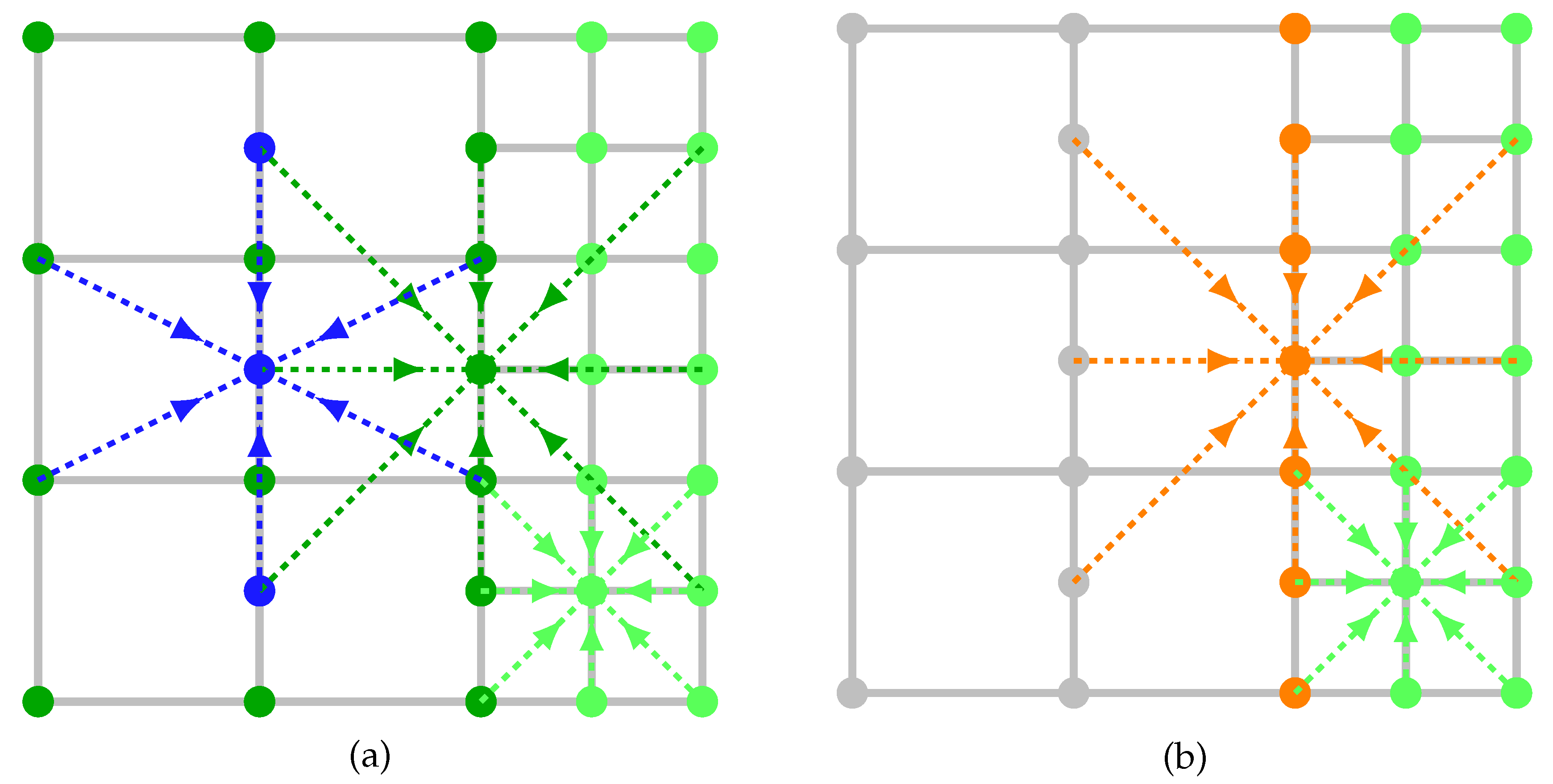
Figure 2.
Grid geometry in the Poiseuille flow benchmark
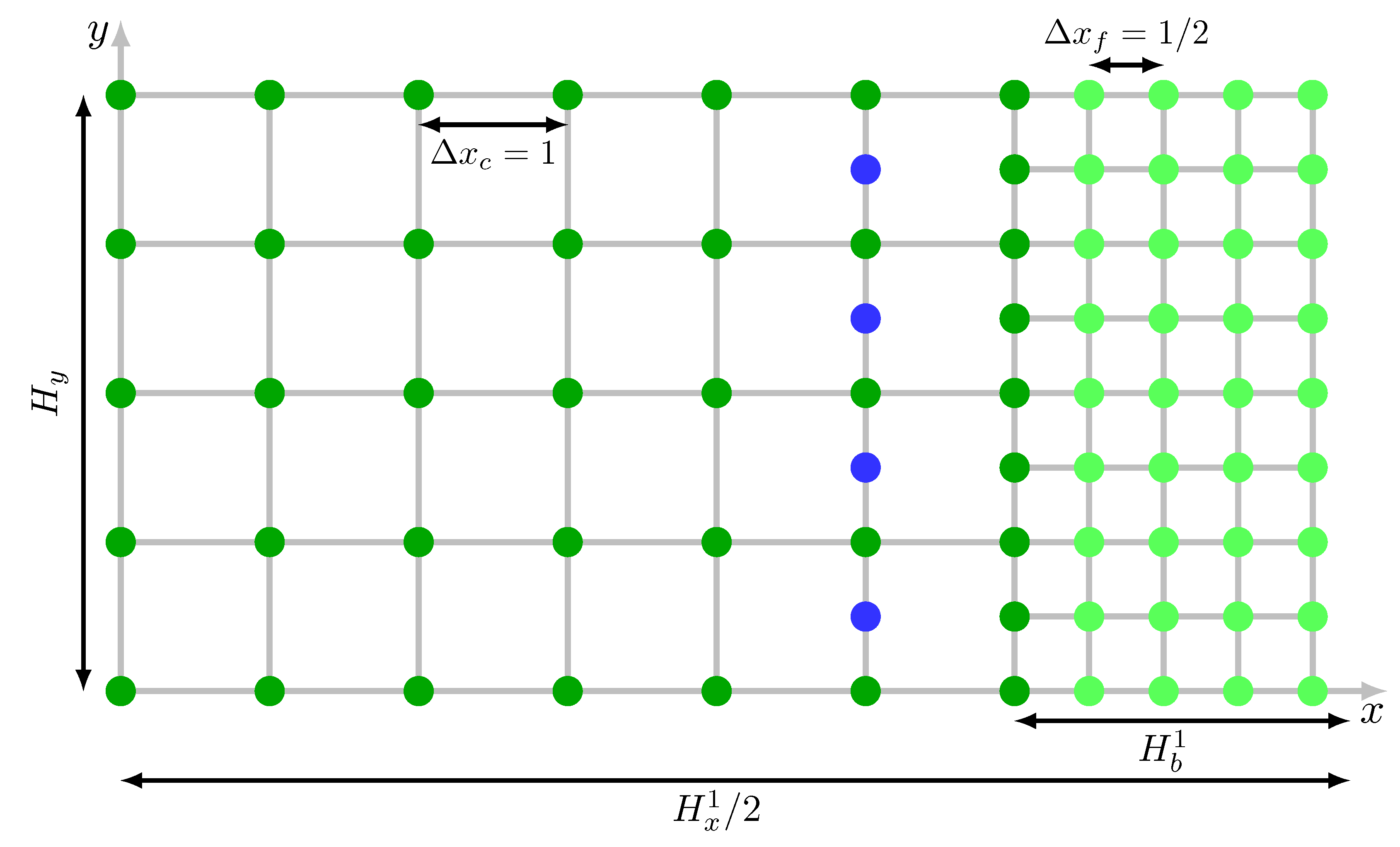
Figure 3.
The , and errors for Poiseuille flow with , .
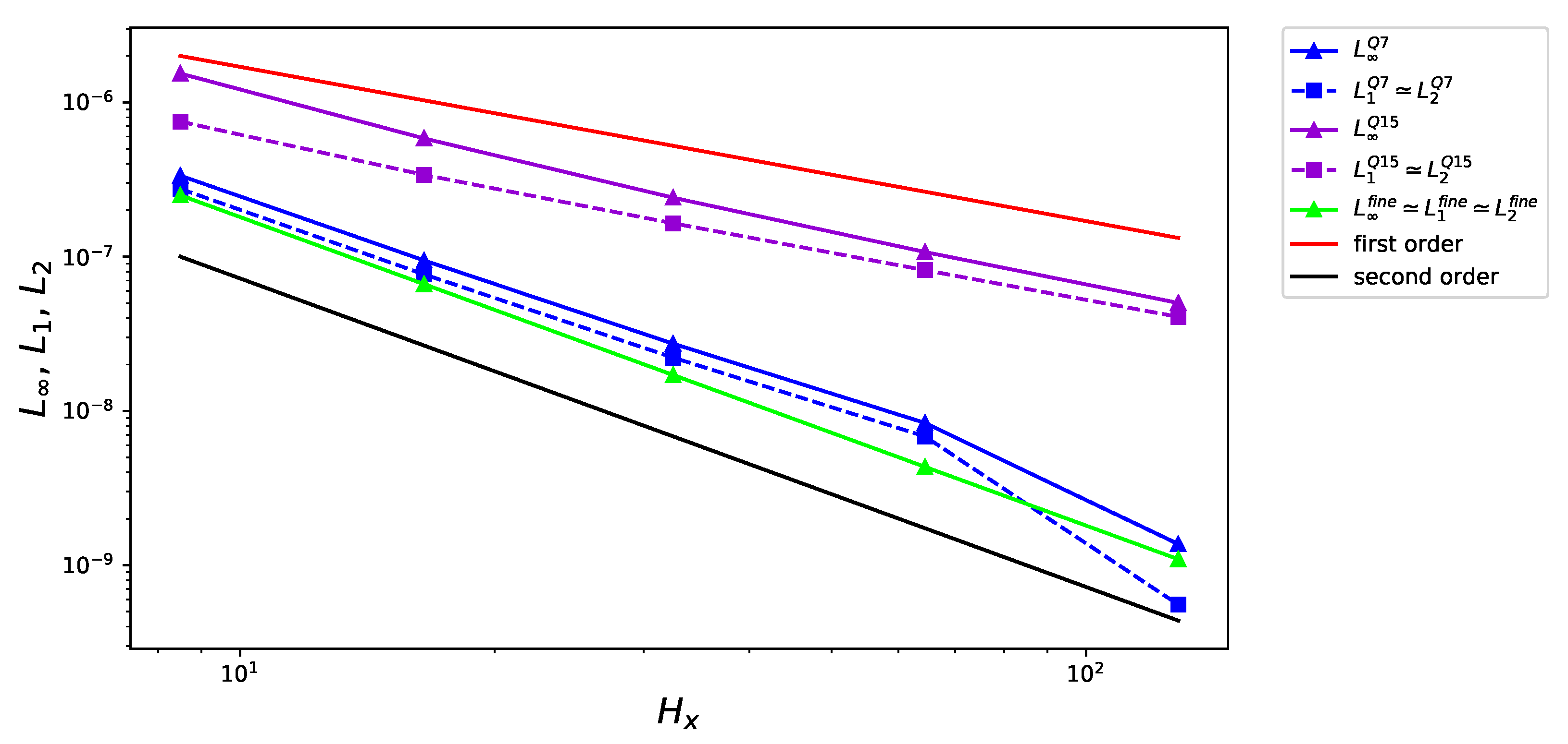
Figure 4.
The , and errors for Poiseuille flow with , .
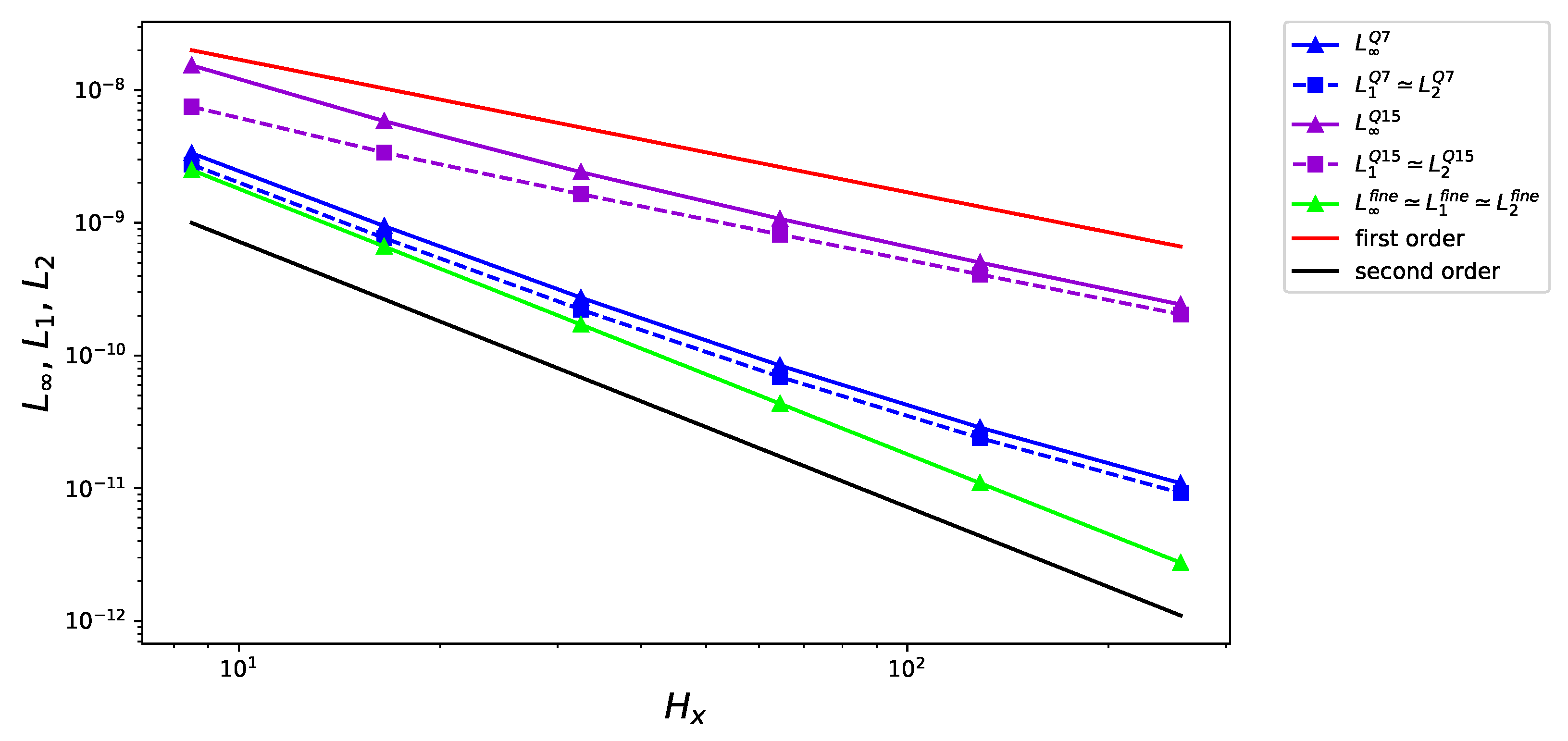
Figure 5.
The absolute error of the Poiseuille flow solution vs the x coordinate. Here, , , .
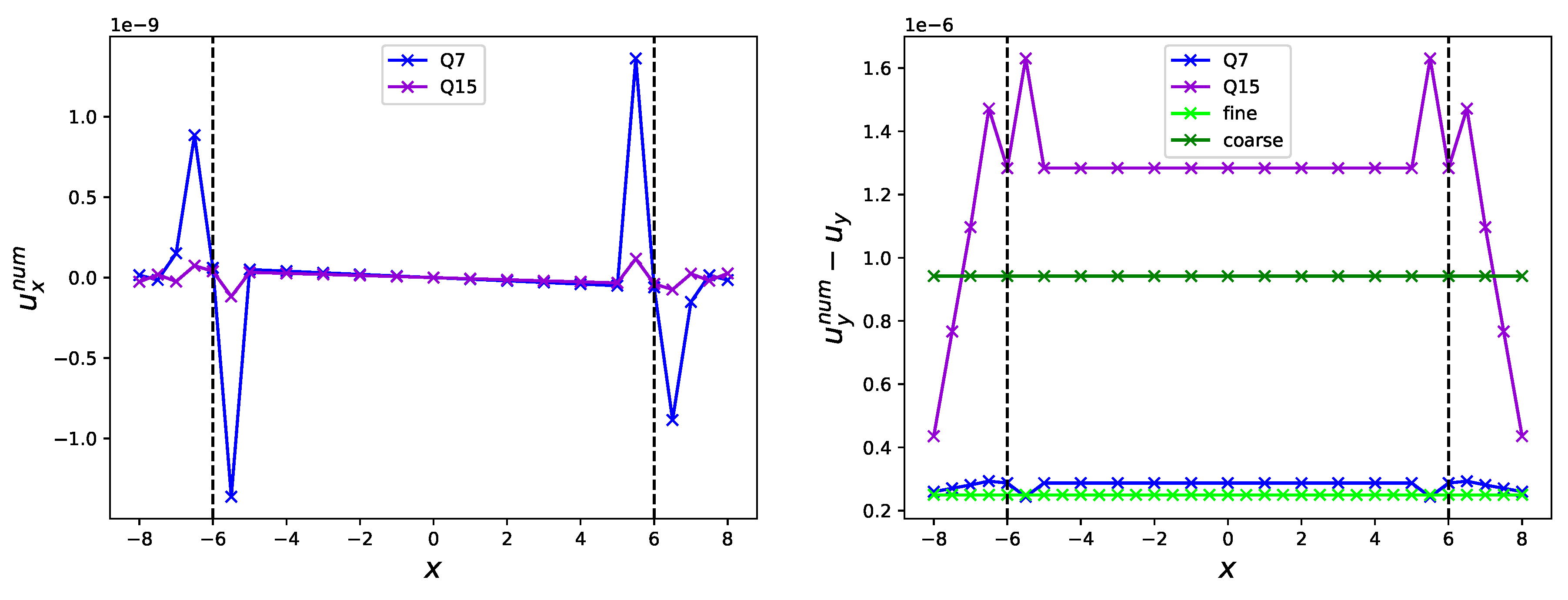
Figure 6.
Vortex density distribution on the color scale at . The grid on the left is refined, and empty spaces in place of the finer nodes on the coarse area are shown in gray color. Left and right image differ in the colormap range.
Figure 6.
Vortex density distribution on the color scale at . The grid on the left is refined, and empty spaces in place of the finer nodes on the coarse area are shown in gray color. Left and right image differ in the colormap range.
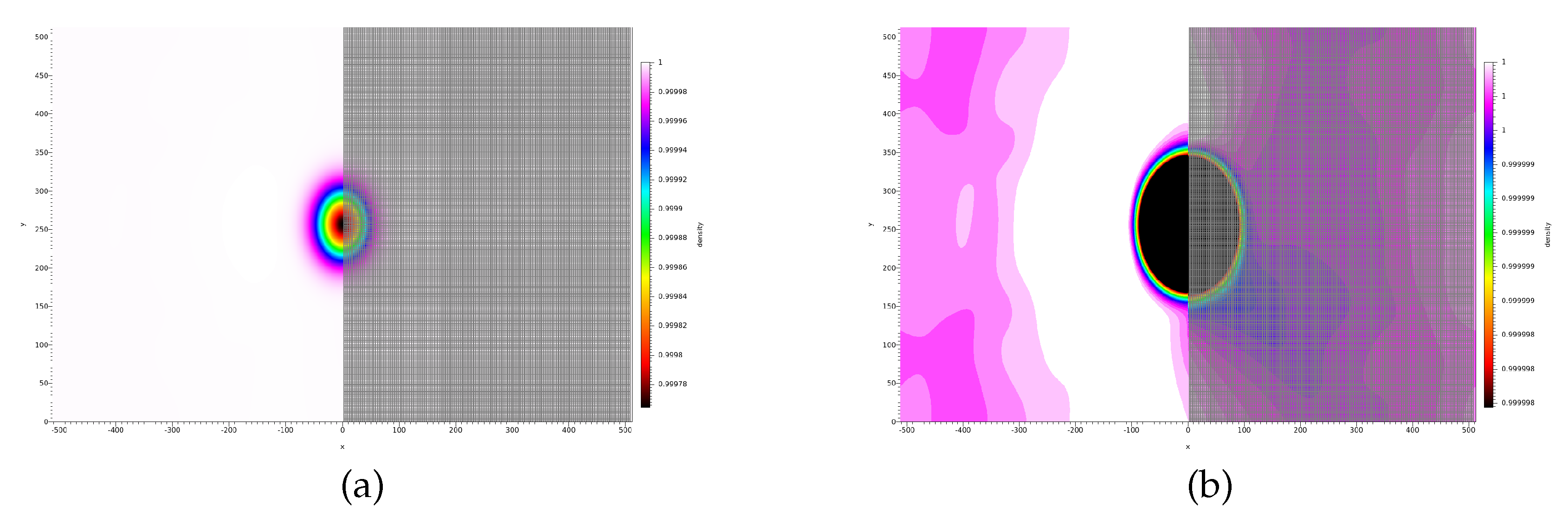
Figure 7.
Density contours for for the 4 time instants.
Disclaimer/Publisher’s Note: The statements, opinions and data contained in all publications are solely those of the individual author(s) and contributor(s) and not of MDPI and/or the editor(s). MDPI and/or the editor(s) disclaim responsibility for any injury to people or property resulting from any ideas, methods, instructions or products referred to in the content. |
© 2023 by the authors. Licensee MDPI, Basel, Switzerland. This article is an open access article distributed under the terms and conditions of the Creative Commons Attribution (CC BY) license (http://creativecommons.org/licenses/by/4.0/).
Copyright: This open access article is published under a Creative Commons CC BY 4.0 license, which permit the free download, distribution, and reuse, provided that the author and preprint are cited in any reuse.


