
Submitted:
12 July 2025
Posted:
15 July 2025
You are already at the latest version
Abstract
This paper investigates the role of Tsallis entropy as a generalized measure of uncertainty in the reliability analysis of consecutive r-out-of-n:G systems, a class of models widely used in engineering applications. We derive new analytical expressions and meaningful bounds for the Tsallis entropy under various lifetime distributions, offering fresh insight into the structural behavior of system-level uncertainty. The approach establishes theoretical connections with classical entropy measures, such as Shannon and Rényi entropies, and provides a foundation for comparing systems under different stochastic orders. A nonparametric estimator is proposed to estimate the Tsallis entropy in this setting, and its performance is evaluated through Monte Carlo simulations. In addition, we develop a new entropy-based test for exponentiality, building on the distinctive properties of system lifetimes. Although Tsallis entropy presents certain limitations, such as non-positivity and lack of additivity, our results support its value as a flexible tool in both reliability characterization and statistical inference.
Keywords:
consecutive r-out-of-n:G systems
; Tsallis entropy
; Shannon entropy
; stochastic orders
; Renyi entropy
1. Introduction
Over the past three decades, consecutive r-out-of-n systems and their variants have attracted significant attention due to their broad applicability across engineering and industrial domains. These systems effectively model real-world configurations such as microwave relay stations in telecommunications, oil pipeline segments, and vacuum assemblies in particle accelerators. Depending on the arrangement and operational logic of the components, several types of consecutive systems can be defined. In particular, a linear consecutive r-out-of-n:G system comprises n components arranged in sequence, where each component is assumed to operate independently and identically (i.i.d.). The system remains functional if at least r consecutive components are operational. Notably, classical series and parallel systems arise as special cases: the series system corresponds to the n-out-of-n:G configuration, while the parallel system aligns with the 1-out-of-nnn:G case. The reliability properties of these systems have been extensively examined under a range of assumptions. Seminal contributions in this area include the works of Jung and Kim [1], Shen and Zuo [2], Kuo and Zuo [3], Chang et al. [4], Boland and Samaniego [5], and Eryılmaz [6,7], among others. Among the various configurations, linear systems that satisfy the condition are of particular interest, as they strike a balance between mathematical tractability and practical applicability in reliability analysis. In these systems, the lifetime of the i-th component is typically denoted by , where i=1,2,…,n. The lifetime of each component is assumed to follow a continuous distribution with probability density function (pdf) , cumulative distribution function (cdf) and survival function . The system lifetime is denoted as . Notably, Eryilmaz [8] showed that when , the reliability function of the consecutive -out-of- :G system is given by:
In information theory, a central objective is to quantify the uncertainty inherent in probability distributions. Within this framework, we focus on the application of Tsallis entropy to consecutive r-out-of-n:G systems, where component lifetimes follow continuous probability distributions. Let be a nonnegative random variable with cumulative distribution function and probability density function . The Tsallis entropy of order , introduced by Tsallis [9], serves as a valuable measure of uncertainty and is defined as:
where , for , represents the quantile function of .
In particular, the Shannon differential entropy, a foundational concept in information theory introduced by Shannon [10], can be obtained as the limiting case of the Tsallis entropy as . Specifically, it is defined by:
An alternative and insightful representation of Tsallis entropy can be derived from Equation (2) by expressing it in terms of the hazard rate function. Specifically, it takes the form:
where represents the hazard rate function, means the expectation, and follows a pdf given by:
It is important to note that Tsallis entropy does not necessarily yield positive values for all . However, remains invariant under location transformations, though it is sensitive to changes in scale. Unlike Shannon entropy, which is additive for independent variables, Tsallis entropy exhibits non-additive behavior. Specifically, for bivariate random variables we have:
The investigation of information-theoretic properties in reliability systems and order statistics has garnered significant scholarly attention. Foundational contributions in this domain include the works of Wong and Chen [11], Park [12], Ebrahimi et al. [13], Zarezadeh and Asadi [14], Toomaj and and Doostparast [15], Toomaj [16] and Mesfioui et al. [17], among others. More recently, Alomani and Kayid [18] explored additional aspects of Tsallis entropy, focusing on coherent and mixed systems under an i.i.d. assumption. Baratpour and Khammar [19] examined its behavior in relation to order statistics and record values, while Kumar [20] studied its role in the context of r-records. Further advancements were made by Kayid and Alshehri [21], who derived an explicit expression for the lifetime entropy of consecutive r-out-of-n:G systems, established a characterization result, proposed practical bounds, and introduced a nonparametric estimator. Complementing this research, Kayid and Shrahili [22] investigated the fractional generalized cumulative residual entropy for similar systems, providing a computational formulation, preservation properties, and two nonparametric estimators supported by empirical validation.
Building upon the existing body of research, this paper aims to further elucidate the role of Tsallis entropy in the analysis of consecutive r-out-of-n:G systems. By extending earlier results, we offer deeper insights into its structural characteristics, propose refined bounding techniques, and develop estimation methods specifically adapted to these reliability models.
The remainder of this paper is organized as follows. Section 2 presents a novel representation for the Tsallis entropy of consecutive r-out-of-n:G systems, denoted by , where component lifetimes are drawn from an arbitrary continuous distribution function F. This representation is derived using the case of the uniform distribution as a baseline. Given the inherent difficulty in deriving exact expressions for Tsallis entropy in complex reliability structures, we address this challenge by establishing several analytical bounds, illustrated through numerical examples. In Section 3, we explore characterization results for Tsallis entropy in the context of consecutive systems, establishing key theoretical properties. Section 4 provides computational evidence supporting our results and introduces a nonparametric estimator tailored for system-level Tsallis entropy. The estimator’s performance is demonstrated using both simulated and real-world data. Finally, Section 5 concludes with a summary of the main findings and their implications.
2. Tsallis Entropy of Consecutive :G System
This section is divided into three main parts. First, we provide a concise review of key results concerning Tsallis entropy and its connections to Rényi and Shannon differential entropies. In the second part, we derive an explicit expression for the Tsallis entropy of a consecutive r-out-of-n:G system and examine its behavior under various stochastic orders. Finally, we present a set of analytical bounds that shed additional light on the entropy structure of these systems.
2.1. Results on Tsallis Entropy
Differential entropy serves as a measure of the average uncertainty associated with a continuous random variable. Broadly speaking, the more a probability density function deviates from the uniform distribution, the higher its differential entropy. In essence, this quantity reflects the expected amount of information gained from observing a specific realization of the random variable. Rényi entropy offers a more flexible framework for quantifying uncertainty compared to differential entropy. For a non-negative random variable with probability density function , Rényi entropy introduces a parameter that enables the exploration of different aspects of uncertainty depending on the weight assigned to various probability outcomes. It is defined as:
The Tsallis and Renyi entropy are also measures of the disparity of the pdf from the uniform distribution. Additionally, these information measures take values in . It is known that for an absolutely continuous nonnegative random variable , we have and . Moreover, one can see that the connection of Renyi and Tsallis entropies is given by and where is defined in (3). In the next theorem, we investigate the relationship of the Shannon differential entropy of proportional hazards rate model defined by (5).
Theorem 2.1.
For an absolutely continuous nonnegative random variable , we have
Proof. By the log-sum inequality, we have
which implies
where denotes the hazard rate function of . By noting that
we get the results for all , and hence the theorem.
2.2. Expression and Stochastic Orders
To obtain the Tsallis entropy expression for the consecutive r-out-of-n:G system, we apply the probability integral transformation It is well known that the transformed variables follow a uniform distribution under certain conditions. Using this transformation, we proceed to obtain an explicit expression for the Tsallis entropy of the system lifetime , assuming that the component lifetimes are independently drawn from a continuous distribution function F. Based on Equation (1), the probability density function of , given by:
Furthermore, when , the pdf of can be represented as follows:
We are now ready to present the following result based on the previous analysis.
Proposition 2.1.
For , the Tsallis entropy of , can be expressed as follows:
where is given by (10).
Proof.
Applying the transformation and referencing Equations (2) and (9), we can obtain the following expressions:
and this completes the proof.
In the subsequent theorem, we present an alternative representation for by employing Newton's generalized binomial theorem and Theorem 2.1.
Theorem 2.2.
Under the conditions of Proposition 2.1, we get
where and for all .
Proof.
By defining and , and referring to (10) and (11), we find that
where the third equality follows directly from Newton's generalized binomial series . This result, in conjunction with Eq. (11), complete the proof.
We now illustrate the utility of the representation in (11) through the following example.
Example 2.1.
Consider a linear consecutive 2-out-of-4:G system with the following lifetime
Let us assume that the component lifetimes are i.i.d. and follow the log-logistic distribution (known as the Fisk distribution in economics). The pdf of this distribution is represented as follows:
After appropriate algebraic manipulation, the following identity is obtained:
As a result of specific algebraic manipulations, we obtain the following expression for the Tsallis entropy:
Due to the difficulty of obtaining a closed-form expression, numerical methods are employed to examine the relationship between and the parameters and . The analysis focuses on the consecutive 2-out-of-4:G system and is carried out for values and , as the integral diverges for and .
As illustrated in Figure 1, the Tsallis entropy decreases as the parameters and increase. This trend reflects the sensitivity of the entropy measure to these parameters and underscores their substantial impact on the system's information-theoretic characteristics.
Definition 2.1.
Let and be two absolutely continuous nonnegative random variables with pdfs and , cdfs and , survival functions and , respectively. Then, (i) is smaller than or equal to in the dispersive order, denoted by , if and only if for all ; (ii) is smaller than in the hazard rate order, denoted by , if is increasing for all ; (iii) it is said to be that exhibits the decreasing failure rate (DFR) property if is decreasing in .
Additional details on these ordering concepts can be found in the comprehensive work of Shaked and Shanthikumar [23]. The following theorem is a direct consequence of the expression given in Equation (11).
Theorem 2.3.
Let and be the lifetimes of two consecutive r-out-of- systems consisting i.i.d. components having cdfs and , respectively. If , then
Proof.
If , then for all , we have
This yields that for all , and this completes the proof.
The following result rigorously demonstrates that, within the class of consecutive r-out-of-n:G systems composed of components with the DFR property, the series system yields the minimum Tsallis entropy.
Proposition 2.2.
Consider the lifetime of a consecutive r-out-of- system, comprising i.i.d. components that exhibit the DFR property. Then, for , and for all ,
- (i). it holds that .
- (ii). it holds that .
Proof.
(i) It is easy to see that . Furthermore, if exhibits the DFR property, then it follows that also possesses the DFR property. Due to Bagai and Kochar [24], it can be concluded that which immediately obtain by recalling Theorem 2.6.
(ii) Based on the findings presented in Proposition 3.2 of Navarro and Eryilmaz [25], it can be inferred that . Consequently, employing analogous reasoning to that employed in Part (i) leads to the acquisition of similar results.
A notable application of Equation (11) lies in comparing the Tsallis entropy of consecutive r-out-of-n:F systems whose components are independent but follow different lifetime distributions, as formalized in the following result.
Proposition 2.3.
Under the conditions of Theorem 2.6, if for all , and , for
then for all and .
Proof.
Given that for all , Equation (2) implies
where . Assuming , based on Equation (11), we have
The first inequality holds because in and in when . The last inequality follows directly from equation (14). Consequently, we have for , which completes the proof for the case . The proof for the case , follows a similar argument.
The following example is provided to illustrate the application of the preceding proposition.
Example 2.2.
Assume coherent systems with lifetimes and , where are i.i.d. component lifetimes with a common cdf , and are i.i.d. component lifetimes with the common cdf . We can easily confirm that and , so . Additionally, since and , we have . Thus Theorem 2.3 implies that
2.3. Some Bounds
In the absence of closed-form expressions for the Tsallis entropy of consecutive systems, particularly when dealing with diverse lifetime distributions or systems comprising a large number of components, bounding techniques become a practical necessity for approximating entropy behavior over the system's lifetime. To address this challenge, the present study examines the role of analytical bounds in characterizing the Tsallis entropy of consecutive r-out-of-n:G systems. Toward this goal, we introduce the following theorem, which provides a lower bound on the Tsallis entropy for such systems. This bound yields valuable insights into entropy dynamics in realistic settings and contributes to a deeper understanding of the underlying system structure.
Lemma 2.1.
Consider a nonnegative continuous random variable with pdf and cdf such that , where , denotes the mode of the pdf . Then, for , we have
Proof.
By noting that , then for , we have . Now, the identity implies that
and hence the result. When , then we have . Now, since , by using the similar arguments, we have the results.
The following theorem establishes a lower bound for the Tsallis entropy of . This bound depends on the Tsallis entropy of a consecutive r-out-of-n:G system under the uniform distribution, as well as the mode of the underlying component lifetime distribution.
Example 2.3.
Assume a linear consecutive -out-of- :G system with lifetime
where for . Let further that the lifetimes of the components are i.i.d. having the common mixture of two Pareto distributions with parameters and with pdf as follows:
Given that the mode of this distribution is , we can determine the mode value as . Consequently, from Lemma 2.1, we get
In the following theorem, we derive bounds for the Tsallis entropy of consecutive r-out-of-n:G systems by leveraging the Tsallis entropy of the individual components.
Theorem 2.4.
When , we have
where where .
Proof.
The mode of is clearly observed as . As a result, we can establish that for . Therefore, for , we can conclude that:
and hence the theorem.
The following example illustrates the lower bound presented in Theorem 2.5 by applying it to a consecutive r-out-of-n:G system.
Example 2.4.
Let us consider a linear consecutive 10-out-of-18:G system with lifetime , where for . In order to conduct the analysis, we assume that the lifetimes of the individual components in the system are i.i.d. according to a common standard exponential distribution. By performing a simple verification, we find that the optimal value is equal to 0.08, resulting in a corresponding value of as 4.268. Utilizing Theorem 2.4, we can write
In the next result, we provide bounds for the consecutive -out-of- :G systems which relates to the hazard rate function of the component lifetimes.
Proposition 2.4.
Let , be the lifetimes of components of a consecutive -out-of- systems with having the common failure rate function . If and . Then
where has the pdf , for .
Proof.
It is easy to see that the hazard rate function of can be expressed as , where
Since for and , it follows that is a monotonically decreasing function of . Given that and , we have for , which implies that , for . Combining this result with the relationship between Tsallis entropy and the hazard rate (as defined in Eq. (4)) for , completes the proof.
Let us consider an illustrative example that demonstrates the application of the preceding proposition.
Example 2.5.
Consider a linear consecutive 2-out-of-3:G system with lifetime , where the component lifetimes are i.i.d. with an exponential distribution with the cdf for . The exponential distribution has a constant hazard rate, , so, it follows that . Applying Proposition 2.4 yields the bounds on the Tsallis entropy of the system as . Based on (11), one can compute the exact value as which falls within the bounds.
The following theorem holds under the assumption that the expected value of the squared hazard rate function of is finite.
Theorem 2.5.
Under the conditions of Theorem 2.11 such that , for and , it holds that
Proof.
The pdf of can be rewritten as , while its failure rate function is given by
Consequently, by (4) and using Cauchy-Schwarz inequality, we obtain
The last equality follows from the change of variable , completing the proof.
3. Characterization Results
In this section, we investigate characterization results for consecutive systems using Tsallis entropy. To illustrate these results, we focus on a specific system type: a linear consecutive ( )-out-of-n:G system, under the condition that , where . To this end, we begin by revisiting a lemma derived from the Müntz–Szász Theorem (as referenced in Kamps [26]), which is commonly used in moment-based characterization theorems.
Lemma 3.1.
For an integrable function on the finite interval ( if 1 , then for almost all , where is a strictly increasing sequence of positive integers satisfying
It is worth pointing out that Lemma 3.1 is a well-established concept in functional analysis, stating that the sets constitutes a complete sequence. Notably, Hwang and Lin [27] expanded the scope of the Müntz-Szász theorem for the functions , where is both absolutely continuous and monotonic over the interval .
Theorem 3.1.
Consider two consecutive ()-out-of-n:G systems with lifetimes and composed of i.i.d. components with cdfs and , and pdfs and , respectively. Then and belong to the same family of distributions, but for a change in location, if and only if for a fixed ,
Proof.
For the necessity part, since and belong to the same family of distributions, but for a change in location, then , for all and . Then, it is clear that
To establish the sufficiency part, we first observe that for a consecutive ( )-out-of- :G system, the following equation holds
where and ranges from 0 to . Given the assumption that , we can write
or equivalently
where
By applying Lemma 3.1 with the function
and considering the complete sequence , one can conclude that
Consequently, and are part of the same distribution family, differing only in a location shift.
Recognizing that a consecutive n-out-of-n:G system is a special case of a series system, the following corollary characterizes its Tsallis entropy.
Corollary 3.1.
Let and be two series systems having the common pdfs and and cdfs and , respectively. Then and belong to the same family of distributions, but for a change in location, if and only if
Another helpful characterization is provided in the following theorem.
Theorem 3.2.
Under the conditions of Theorem 3.1, and belong to the same family of distributions, but for a change in location and scale, if and only if for a fixed ,
Proof.
The necessity is straightforward, so we must now establish the sufficiency aspect. Leveraging Eqs. (6) and (18), we can derive
An analogous argument can be made for . If relation (22) holds for two cdfs and , then we can infer from Equation (23) that
Let us set . Using similar arguments as in the proof of Theorem 3.2, we can write
The proof is then completed by using similar arguments to those in Theorem 3.2.
By applying Theorem 3.2, we derive the following corollary.
Corollary 3.2.
Suppose the assumptions of Corollary 3.1, and belong to the same family of distributions, but for a change in location and scale, if and only if for a fixed ,
The exponential distribution is characterized in the following theorem through the use of Tsallis entropy for consecutive r-out-of-n:G systems. This result serves as the theoretical basis for a newly developed goodness-of-fit test for the exponential distribution, applicable to a wide range of datasets. To establish this result, we begin by introducing the lower incomplete beta function, defined as:
where and are positive real numbers. When this expression reduces to the complete beta function. We now proceed to present the main result.
Theorem 3.3.
Let us assume that is the lifetime of the consecutive -out-of-n:G system having i.i.d. component lifetimes with the pdf and . Then has an exponential distribution with the parameter if and only if for a fixed ,
for all , and .
Proof.
Given an exponentially distributed random variable , its Tsallis entropy, directly calculated using , is . Furthermore, since , application of Eq. (11) yields:
for . To derive the second term, let us set and , uponrecalling (10), it holds that
where the necessity is derived. To establish sufficiency, we assume that Equation (25) holds for a fixed value of and assume that . Following the proof of Theorem 3.1 and utilizing the result in Equation (26), we obtain the following relation
which is equivalent to
where is defined in (18). Thus, it holds that
where is defined in (21). Applying Lemma 3.1 to the function
and utilizing the complete sequence , we can deduce that
This implies that
By solving this equation, it yields , where is an arbitrary constant. Utilizing the boundary condition , it follows that , we determine that . Consequently, leading to for . This implies the cdf , confirming that follows an exponential distribution with scale parameter . This establishes the theorem.
4. Entropy-Based Exponentiality Testing
In this section, we introduce a nonparametric method for estimating the Tsallis entropy of consecutive r-out-of-n:G systems. The exponential distribution’s broad applicability has led to the development of numerous test statistics aimed at assessing exponentiality. These methods often rely on foundational principles in statistical theory. The central objective here is to determine whether the distribution of a random variable T follows an exponential distribution. Let denote the cdf of the exponential distribution, defined as , for . The hypothesis under investigation is stated as follows:
Extropy has recently gained considerable attention in the research community as a useful metric for goodness-of-fit testing. Qiu and Jia [28] pioneered the development of two consistent estimators for Tsallis entropy based on the concept of spacings and subsequently constructed a goodness-of-fit test for the uniform distribution using the more efficient of the two. In a related contribution, Xiong et al. [29] exploited the properties of classical record values to derive a characterization result for the exponential distribution, leading to the development of a novel exponentiality test. Their work carefully outlined the test statistic and emphasized its strong performance, particularly with small sample sizes. Building on this foundation, Jose and Sathar [30] proposed a new exponentiality test based on a characterization involving the Tsallis entropy of lower r-record values.
The present section aims to extend these developments by exploring the Tsallis entropy of consecutive r-out-of-n:G systems. As established in Theorem 3.3, the exponential distribution can be uniquely characterized through the Tsallis entropy associated with such systems. Leveraging Equation (25) and after simplification, we propose a new test statistic for the exponentiality, denoted by , and for , defined as follows:
where
then Theorem 3.3 directly implies that if and only if is exponentially distributed. This fundamental property establishes as a viable measure of exponentiality and a suitable candidate for a test statistic. Given a random sample , an estimator of can be used as a test statistic. Significant deviations of from its expected value under the null hypothesis (i.e., the assumption of an exponential distribution) would indicate non-exponentiality, prompting the rejection of the null hypothesis. Consider a random sample of size , denoted by drawn from an absolutely continuous distribution and represent the corresponding order statistics. To estimate the test statistic, we adopt an estimator proposed by Vasicek [31] for as follows:
and is a positive integer smaller than which is known as the window size and for and for . So, a reasonable estimator for can be derived using Equation (30) as follows:
Establishing the consistency of an estimator is essential, particularly when evaluating estimators for parametric functions. The following theorem confirms the result stated in Equation (25). The proof adopts an approach similar to that of Theorem 1 in Vasicek's [31]. Notably, Park [32] and Xiong et al. [29] also utilized the consistency proof technique introduced by Vasicek [31] to validate the reliability of their respective test statistics.
Theorem 4.1.
Assume that is a random sample of size taken from a population with pdf and cdf . Also, let the variance of the random variable be finite. Then as and , where stands for the convergence in probability for all .
Proof.
To establish the consistency of the estimator , we employ the approach given in Noughabi and Arghami [33]. As both and tend to infinity, with the ratio approaching 0, we can approximate the density as follows:
where represents the empirical distribution function. Furthermore, given that , we can express
where the second approximation relies on the almost sure convergence of the empirical distribution function i.e. as . Now, applying the Strong Law of Large Numbers, we have
This convergence demonstrates that is a consistent estimator of and hence completes the proof of consistency for all .
The following theorem shows that the root mean square error (RMSE) of remains invariant under location shifts in the random variable T. However, this invariance does not hold under scale transformations. The proof of these results can be obtained by adapting the arguments presented by Ebrahimi et al. [34].
Theorem 4.2.
Assume that is a random sample of size taken from a population with pdf and and . Denote the estimators for on the basis of and with and , respectively. Then, the following properties apply:
- 3.
- ,
- 4.
- ,
- 5.
- , for all .
Proof.
It is not hard to see from (25) that
The proof is then completed by leveraging the properties of the mean, variance, and RMSE of .
Various combinations of n and i can be used to construct a range of test statistics. For computational purposes, we choose and which simplifies the expression in Equation (30) for evaluation. Under the null hypothesis, , the value of asymptotically converges to zero as the sample size approaches infinity. Conversely, under an alternative distribution with an absolutely continuous cdf , the value of converges to a positive value as . Based on these asymptotic properties, we reject the null hypothesis at a given significance level , for a finite sample size if the observed value of the test statistic exceeds the critical value . The asymptotic distribution of is intricate and analytically intractable due to its dependence on both the sample size and the window parameter .
To overcome this, we employed a Monte Carlo simulation approach. Specifically, we generated 10,000 samples of sizes from the standard exponential distribution under the null hypothesis. For each sample size, we determined the -th quantile of the simulated values to establish the critical value for significance levels , while varying the window size from 2 to 30. Table 1 and Table 2 present the resulting critical values for the respective sample sizes and significance levels.
Power Comparisons
The power of the test was assessed through a Monte Carlo simulation involving nine alternative probability distributions. For each sample size replicates of size N were drawn from each alternative distribution, and the statistic was computed for each. The power at a significance level was then estimated as the empirical rejection rate, specifically the proportion of the 10,000 samples yielding a statistic exceeding the critical threshold.
To validate the efficiency of the newly introduced test based on the statistic, its performance will be benchmarked against several existing tests for exponentiality reported in the literature, with the specifications of the alternative distributions provided in Table 3.
The simulation setup, including the selection of alternative distributions and their parameters, closely follows the methodology proposed by Jose and Sathar [30]. To assess the efficiency of the newly proposed test based on the statistic, its performance is compared with several established tests for exponentiality reported in the literature, as summarized in Table 4.
The performance of the statistic is contingent upon the window size m, necessitating the prior determination of an appropriate value to ensure adequate adjusted statistical power. Simulations across varying sample sizes resulted in the heuristic formula , where is the floor function. This formula provides a practical guideline for selecting and aims to ensure robust power performance across different distributions.
To comprehensively assess the performance of the proposed , test, we selected ten established tests for exponentiality and evaluated their power against a diverse set of alternative distributions. Notably, Xiong et al. [29] introduced a test statistic based on the Tsallis entropy of classical record values, while Jose and Sathar [30] characterized the exponential distribution using Tsallis entropy derived from lower iii-records and developed a corresponding test statistic.
These two tests, designated as and in Table 4, are included in our comparative analysis due to their foundation in information-theoretic principles. The original authors provided detailed discussions supporting their relevance and applicability for testing exponentiality. To estimate the power of each test, we simulated 10,000 independent samples for each sample size from each alternative distribution detailed in Table 3. The power values for the , test was then computed at a 5 percent significance level. Subsequently, the power values for , and the eleven competing tests were calculated for the same sample sizes and alternative distributions. These comparative results are summarized in Table 5.
In general, the test statistic demonstrates strong performance in detecting deviations from exponentiality towards the gamma distribution. However, its performance against other alternative distributions, including Weibull, uniform, half-normal, and log-normal, is moderate, exhibiting neither exceptional strength nor significant weakness.
5. Conclusions
This study explores the role of Tsallis entropy within the framework of consecutive r-out-of-n:G systems. A key contribution lies in identifying a meaningful connection between the Tsallis entropy of systems with general continuous lifetime distributions and those governed by the uniform distribution. Given the challenges of deriving closed-form entropy expressions, especially in systems with large n or complex component distributions, we propose a set of informative bounds that offer practical approximations. These bounds enhance both the theoretical understanding and empirical analysis of Tsallis entropy in reliability contexts. Furthermore, we develop a nonparametric estimator specifically tailored for consecutive r-out-of-n:G systems and demonstrate its effectiveness using simulated and real data. The estimator provides valuable insights into system-level uncertainty and reliability, with potential applications in fields such as image processing, where entropy-based measures support data-driven decision-making.
In summary, this work advances the application of Tsallis entropy in reliability modeling by (i) establishing theoretical relationships, (ii) deriving practical bounds, and (iii) introducing a robust estimation technique. These contributions lay the foundation for future research into entropy-based methodologies across a wide range of statistical and engineering domains.
Data Availability
The datasets are available within the manuscript.
Acknowledgments
Princess Nourah bint Abdulrahman University Researchers Supporting Project number (PNURSP2025R226), Princess Nourah bint Abdulrahman University, Riyadh, Saudi Arabia.
Conflicts of interest
The authors declare that they have no conflicts of interest to report regarding the present study.
References
- Jung, K.-H.; Kim, H. Linear consecutive-k-out-of-n:F system reliability with common-mode forced outages. Reliab. Eng. Syst. Saf. 1993, 41, 49–55. [Google Scholar] [CrossRef]
- Shen, J.; Zuo, M.J. Optimal design of series consecutive-k-out-of-n:G systems. Reliab. Eng. Syst. Saf. 1994, 45, 277–283. [Google Scholar] [CrossRef]
- Kuo, W.; Zuo, M.J. Optimal Reliability Modeling: Principles and Applications; John Wiley & Sons, 2003. [Google Scholar]
- Chung, C.I.-H.; Cui, L.; Hwang, F.K. Reliabilities of Consecutive-k Systems; Springer, 2013; Vol. 4. [Google Scholar]
- Boland, P.J.; Samaniego, F.J. Stochastic ordering results for consecutive k-out-of-n:F systems. IEEE Trans. Reliab. 2004, 53, 7–10. [Google Scholar] [CrossRef]
- Eryılmaz, S. Mixture representations for the reliability of consecutive-k systems. Math. Comput. Model. 2010, 51, 405–412. [Google Scholar] [CrossRef]
- Eryılmaz, S. Conditional lifetimes of consecutive k-out-of-n systems. IEEE Trans. Reliab. 2010, 59, 178–182. [Google Scholar] [CrossRef]
- Eryılmaz, S. Reliability properties of consecutive k-out-of-n systems of arbitrarily dependent components. Reliab. Eng. Syst. Saf. 2009, 94, 350–356. [Google Scholar] [CrossRef]
- Tsallis, C. Possible generalization of Boltzmann-Gibbs statistics. J. Stat. Phys. 1988, 52, 479–487. [Google Scholar] [CrossRef]
- Shannon, C.E. A mathematical theory of communication. Bell Syst. Tech. J. 1948, 27, 379–423. [Google Scholar] [CrossRef]
- Wong, K.M.; Chen, S. The entropy of ordered sequences and order statistics. IEEE Trans. Inf. Theory 1990, 36, 276–284. [Google Scholar] [CrossRef]
- Park, S. The entropy of consecutive order statistics. IEEE Trans. Inf. Theory 1995, 41, 2003–2007. [Google Scholar] [CrossRef]
- Ebrahimi, N.; Soofi, E.S.; Soyer, R. Information measures in perspective. Int. Stat. Rev. 2010, 78, 383–412. [Google Scholar] [CrossRef]
- Zarezadeh, S.; Asadi, M. Results on residual Rényi entropy of order statistics and record values. Inf. Sci. 2010, 180, 4195–4206. [Google Scholar] [CrossRef]
- Toomaj, A.; Doostparast, M. A note on signature-based expressions for the entropy of mixed r-out-of-n systems. Naval Res. Logist. 2014, 61, 202–206. [Google Scholar] [CrossRef]
- Toomaj, A. Rényi entropy properties of mixed systems. Commun. Stat. Theory Methods 2017, 46, 906–916. [Google Scholar] [CrossRef]
- Mesfioui, M.; Kayid, M.; Shrahili, M. Rényi entropy of the residual lifetime of a reliability system at the system level. Axioms 2023, 12, 320. [Google Scholar] [CrossRef]
- Alomani, G.; Kayid, M. Further properties of Tsallis entropy and its application. Entropy 2023, 25, 199. [Google Scholar] [CrossRef]
- Baratpour, S.; Khammar, A.H. Results on Tsallis entropy of order statistics and record values. Istatistik J. Turk. Stat. Assoc. 2016, 8, 60–73. [Google Scholar]
- Kumar, V. Some results on Tsallis entropy measure and k-record values. Physica A 2016, 462, 667–673. [Google Scholar] [CrossRef]
- Kayid, M.; Alshehri, M.A. Shannon differential entropy properties of consecutive k-out-of-n:G systems. Oper. Res. Lett. 2024, 57, 107190. [Google Scholar] [CrossRef]
- Kayid, M.; Shrahili, M. Information properties of consecutive systems using fractional generalized cumulative residual entropy. Fractal Fract. 2024, 8(10), 568. [Google Scholar] [CrossRef]
- Shaked, M.; Shanthikumar, J.G. Stochastic Orders; Springer, 2007. [Google Scholar]
- Bagai, I.; Kochar, S.C. On tail-ordering and comparison of failure rates. Commun. Stat. Theory Methods 1986, 15, 1377–1388. [Google Scholar] [CrossRef]
- Navarro, J.; Eryilmaz, S. Mean residual lifetimes of consecutive-k-out-of-n systems. J. Appl. Probab. 2007, 44, 82–98. [Google Scholar] [CrossRef]
- Kamps, U. Characterizations of distributions by recurrence relations and identities for moments of order statistics. In Handbook of Statistics; 1998; Volume 16, pp. 291–311. [Google Scholar]
- Hwang, J.S.; Lin, G.D. On a generalized moment problem. II. Proc. Amer. Math. Soc. 1984, 91, 577–580. [Google Scholar] [CrossRef]
- Qiu, G.; Jia, K. Extropy estimators with applications in testing uniformity. J. Nonparametr. Stat. 2018, 30, 182–196. [Google Scholar] [CrossRef]
- Xiong, P.; Zhuang, W.; Qiu, G. Testing exponentiality based on the extropy of record values. J. Appl. Stat. 2022, 49, 782–802. [Google Scholar] [CrossRef] [PubMed]
- Jose, J.; Sathar, E.I.A. Characterization of exponential distribution using extropy based on lower k-records and its application in testing exponentiality. J. Comput. Appl. Math. 2022, 402, 113816. [Google Scholar] [CrossRef]
- Vasicek, O. A test for normality based on sample entropy. J. R. Stat. Soc. Ser. B Stat. Methodol. 1976, 38, 54–59. [Google Scholar] [CrossRef]
- Park, S. A goodness-of-fit test for normality based on the sample entropy of order statistics. Stat. Probab. Lett. 1999, 44, 359–363. [Google Scholar] [CrossRef]
- Hadi Alizadeh Noughabi and Naser Reza Arghami. Testing exponentiality based on characterizations of the exponential distribution. Journal of Statistical Computation and Simulation 2011, 81, 1641–1651. [Google Scholar] [CrossRef]
- Ebrahimi, N.; Pflughoeft, K.; Soofi, E.S. Two measures of sample entropy. Stat. Probab. Lett. 1994, 20, 225–234. [Google Scholar] [CrossRef]
- Fortiana, J.; Grané, A. A scale-free goodness-of-fit statistic for the exponential distribution based on maximum correlations. J. Stat. Plann. Inference 2002, 108, 85–97. [Google Scholar] [CrossRef]
- Choi, B.; Kim, K.; Song, S.H. Goodness-of-fit test for exponentiality based on Kullback-Leibler information. Commun. Stat. Simul. Comput. 2004, 33, 525–536. [Google Scholar] [CrossRef]
- Mimoto, N.; Zitikis, R. The Atkinson index, the Moran statistic, and testing exponentiality. J. Jpn. Stat. Soc. 2008, 38, 187–205. [Google Scholar] [CrossRef]
- Volkova, K.Y. On asymptotic efficiency of exponentiality tests based on Rossberg's characterization. J. Math. Sci. 2010, 167, 489–493. [Google Scholar] [CrossRef]
- Zamanzade, E.; Arghami, N.R. Goodness-of-fit test based on correcting moments of modified entropy estimator. J. Stat. Comput. Simul. 2011, 81, 2077–2093. [Google Scholar] [CrossRef]
- Baratpour, S.; Rad, A.H. Testing goodness-of-fit for exponential distribution based on cumulative residual entropy. Commun. Stat. Theory Methods 2012, 41, 1387–1396. [Google Scholar] [CrossRef]
- Noughabi, H.A.; Arghami, N.R. Goodness-of-fit tests based on correcting moments of entropy estimators. Commun. Stat. Simul. Comput. 2013, 42, 499–513. [Google Scholar] [CrossRef]
- Volkova, K.Y.; Nikitin, Y.Y. Exponentiality tests based on Ahsanullah’s characterization and their efficiency. J. Math. Sci. 2015, 204, 42–54. [Google Scholar] [CrossRef]
- Torabi, H.; Montazeri, N.H.; Grané, A. A wide review on exponentiality tests and two competitive proposals with application on reliability. J. Stat. Comput. Simul. 2018, 88, 108–139. [Google Scholar] [CrossRef]
Figure 1.
The plot of with respect to and as demonstrated in Example 2.1.
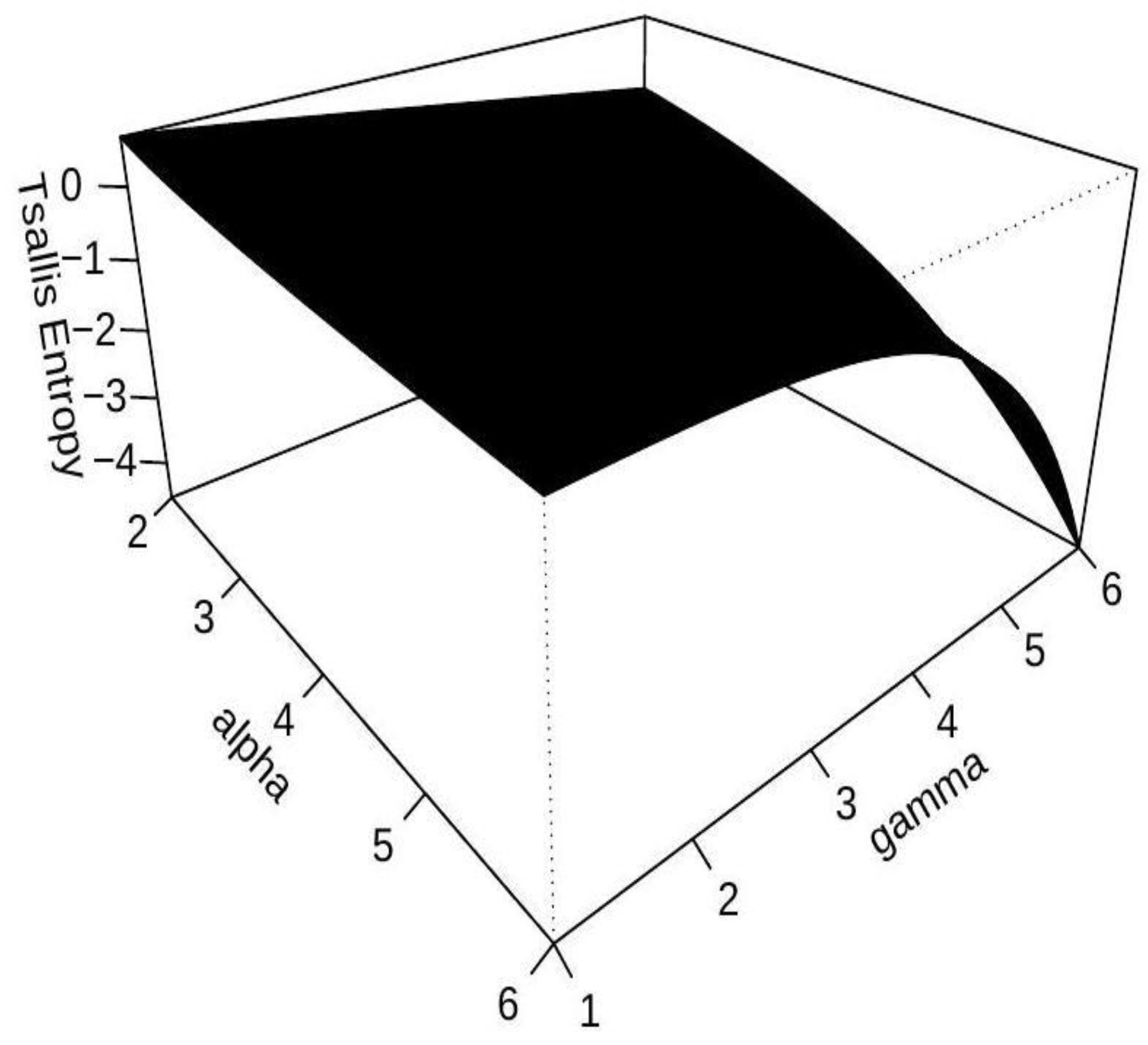

Table 1.
Critical values of the statistic at significance level .
| 2 | 3.314111 | 4.885299 | 5.31386 | 5.669357 | 5.665471 | 5.879007 | 5.969947 |
| 3 | 2.958639 | 3.575905 | 3.652558 | 3.735460 | 3.929436 | 3.934263 | |
| 4 | 2.091046 | 2.584478 | 2.745547 | 2.981776 | 3.072066 | 3.135100 | |
| 5 | 2.209270 | 2.462253 | 2.569272 | 2.619691 | 2.657987 | ||
| 6 | 1.960857 | 2.129584 | 2.283690 | 2.277793 | 2.414754 | ||
| 7 | 1.734072 | 1.992837 | 2.066112 | 2.116888 | 2.232844 | ||
| 8 | 1.609901 | 1.819573 | 1.922531 | 1.975798 | 2.081751 | ||
| 9 | 1.455605 | 1.673973 | 1.802262 | 1.858107 | 1.945239 | ||
| 10 | 1.587775 | 1.675985 | 1.782838 | 1.877756 | |||
| 11 | 1.488481 | 1.620426 | 1.688339 | 1.848637 | |||
| 12 | 1.416203 | 1.538009 | 1.614312 | 1.764357 | |||
| 13 | 1.342485 | 1.472354 | 1.577332 | 1.722066 | |||
| 14 | 1.285730 | 1.406798 | 1.500436 | 1.675081 | |||
| 15 | 1.369318 | 1.455467 | 1.629516 | ||||
| 16 | 1.322761 | 1.420537 | 1.607517 | ||||
| 17 | 1.271932 | 1.372767 | 1.574213 | ||||
| 18 | 1.233146 | 1.339279 | 1.523170 | ||||
| 19 | 1.195628 | 1.308735 | 1.499460 | ||||
| 20 | 1.259018 | 1.476491 | |||||
| 21 | 1.226252 | 1.436125 | |||||
| 22 | 1.203902 | 1.419521 | |||||
| 23 | 1.166646 | 1.396562 | |||||
| 24 | 1.137062 | 1.382412 | |||||
| 25 | 1.367450 | ||||||
| 26 | 1.326762 | ||||||
| 27 | 1.313035 | ||||||
| 28 | 1.301748 | ||||||
| 29 | 1.274347 | ||||||
| 30 | 1.268577 |
Table 2.
Critical values of the statistic at significance level .
| 2 | 7.741372 | 11.020993 | 13.130953 | 14.345684 | 14.343766 | 14.219676 | 13.504338 |
| 3 | 5.330965 | 6.404442 | 7.433630 | 6.808109 | 6.722751 | 7.335729 | |
| 4 | 3.388231 | 4.296331 | 4.723610 | 4.846727 | 4.829120 | 5.240127 | |
| 5 | 3.316372 | 3.695920 | 3.789253 | 3.926883 | 4.006127 | ||
| 6 | 2.804852 | 3.208528 | 3.263101 | 3.443553 | 3.478685 | ||
| 7 | 2.548659 | 2.771682 | 2.937497 | 2.903739 | 3.083877 | ||
| 8 | 2.211149 | 2.461236 | 2.679584 | 2.677176 | 2.844005 | ||
| 9 | 1.992974 | 2.214899 | 2.379238 | 2.401170 | 2.585907 | ||
| 10 | 2.071670 | 2.276676 | 2.272026 | 2.477653 | |||
| 11 | 1.905570 | 2.009089 | 2.231709 | 2.328932 | |||
| 12 | 1.827860 | 2.002682 | 2.037605 | 2.226634 | |||
| 13 | 1.681670 | 1.860946 | 1.978671 | 2.171389 | |||
| 14 | 1.594050 | 1.808541 | 1.853613 | 2.038638 | |||
| 15 | 1.700383 | 1.812322 | 1.999786 | ||||
| 16 | 1.642237 | 1.733522 | 1.956928 | ||||
| 17 | 1.541187 | 1.671427 | 1.873484 | ||||
| 18 | 1.485475 | 1.589422 | 1.864797 | ||||
| 19 | 1.439565 | 1.549233 | 1.800001 | ||||
| 20 | 1.520203 | 1.777315 | |||||
| 21 | 1.477773 | 1.733554 | |||||
| 22 | 1.435841 | 1.678109 | |||||
| 23 | 1.380899 | 1.637635 | |||||
| 24 | 1.341584 | 1.646366 | |||||
| 25 | 1.574026 | ||||||
| 26 | 1.563578 | ||||||
| 27 | 1.526702 | ||||||
| 28 | 1.512871 | ||||||
| 29 | 1.481510 | ||||||
| 30 | 1.462325 |
Table 3.
Alternative Probability Distributions for Evaluating the Power of the Test Statistic.
| Distribution | Probability Density Function | Support | Notation |
| Weibull | , | ||
| Gamma | |||
| Uniform | , | ||
| Half-Normal | , | ||
| Log-Normal | , |
Table 4.
Competing Tests for Exponentiality.
| Test | Reference | Notation |
| 1 | Fortiana and Grané [35] | |
| 2 | Choi et al. [36] | |
| 3 | Mimoto and Zitikis [37] | |
| 4 | Volkova [38] | |
| 5 | Zamanzade and Arghami [39] | |
| 6 | Baratpour and Rad [40] | |
| 7 | Noughabi and Arghami [41] | |
| 8 | Volkova and Nikitin [42] | |
| 9 | Torabi et al. [43] | |
| 10 | Xiong et al. [29] | |
| 11 | Jose and Sathar [30] |
Table 5.
Power comparisons of the tests in significance level
| 10 | 5 | 5 | 5 | 5 | 5 | 5 | 5 | 5 | 5 | 5 | 5 | 5 | |
| 34 | 11 | 50 | 46 | 29 | 7 | 0 | 50 | 65 | 60 | 83 | 75 | ||
| 15 | 17 | 16 | 13 | 16 | 23 | 29 | 16 | 1 | 15 | 17 | 3 | ||
| 11 | 10 | 10 | 8 | 10 | 8 | 20 | 10 | 1 | 18 | 8 | 5 | ||
| 42 | 28 | 31 | 15 | 33 | 60 | 51 | 24 | 2 | 93 | 100 | 10 | ||
| 12 | 24 | 16 | 21 | 23 | 17 | 26 | 19 | 2 | 5 | 5 | 2 | ||
| 36 | 19 | 40 | 6 | 29 | 15 | 1 | 9 | 47 | 3 | 2 | 3 | ||
| 20 | 5 | 5 | 5 | 5 | 5 | 5 | 5 | 5 | 6 | 5 | 5 | 5 | |
| 56 | 31 | 77 | 80 | 66 | 25 | 0 | 82 | 89 | 95 | 99 | 96 | ||
| 32 | 27 | 34 | 27 | 17 | 33 | 47 | 29 | 6 | 29 | 8 | 2 | ||
| 23 | 14 | 19 | 12 | 7 | 30 | 23 | 14 | 2 | 37 | 5 | 4 | ||
| 86 | 52 | 63 | 28 | 54 | 92 | 80 | 39 | 18 | 100 | 100 | 12 | ||
| 18 | 52 | 26 | 48 | 42 | 18 | 49 | 45 | 8 | 4 | 4 | 0 | ||
| 61 | 45 | 67 | 11 | 64 | 43 | 0 | 16 | 71 | 0 | 3 | 2 | ||
| 50 | 5 | 5 | 5 | 5 | 5 | 5 | 5 | 5 | 5 | 5 | 5 | 5 | |
| 89 | 78 | 99 | 99 | 95 | 68 | 0 | 99 | 100 | 100 | 100 | 100 | ||
| 73 | 55 | 79 | 65 | 5 | 62 | 80 | 67 | 37 | 56 | 7 | 0 | ||
| 59 | 23 | 52 | 25 | 1 | 54 | 48 | 28 | 13 | 73 | 2 | 2 | ||
| 100 | 91 | 98 | 62 | 62 | 100 | 99 | 72 | 78 | 100 | 100 | 24 | ||
| 26 | 93 | 44 | 93 | 55 | 24 | 84 | 92 | 47 | 3 | 3 | 0 | ||
| 93 | 85 | 95 | 25 | 93 | 85 | 0 | 29 | 95 | 0 | 2 | 0 |
Disclaimer/Publisher’s Note: The statements, opinions and data contained in all publications are solely those of the individual author(s) and contributor(s) and not of MDPI and/or the editor(s). MDPI and/or the editor(s) disclaim responsibility for any injury to people or property resulting from any ideas, methods, instructions or products referred to in the content. |
© 2025 by the authors. Licensee MDPI, Basel, Switzerland. This article is an open access article distributed under the terms and conditions of the Creative Commons Attribution (CC BY) license (http://creativecommons.org/licenses/by/4.0/).
Copyright: This open access article is published under a Creative Commons CC BY 4.0 license, which permit the free download, distribution, and reuse, provided that the author and preprint are cited in any reuse.


