

Submitted:
18 August 2024
Posted:
20 August 2024
You are already at the latest version
Abstract
This paper reveals some properties of the cumulative entropy of consecutive k-out-of-n:F
system's lifetime. First, we introduce a method for calculating the cumulative entropy of
their lifetime and explore its preservation properties using established stochastic orders. Ad-
ditionally, we obtain useful bounds that can used in situations where the distribution function
of the system's component lifetimes are complicated or systems have large components. To
support practical applications, we present two nonparametric estimators for the cumulative
entropy of these systems. The efficiency and performance of these estimators are illustrated
with simulated datasets and further validated with real data sets.
Keywords:
Consecutive k-out-of-n:F systems
; Cumulative entropy
; Shannon entropy
; Stochas- tic orders
; Real data
1. Introduction
Over the past three decades, extensive research has focused on k-out-of-n systems with consecutive structure and their different variations. A consecutive k-out-of-n system can be classified by the arrangement of its components as either linear or circular, and by its functioning principle as either a failure or a good system. A linear consecutive k-out-of-n:F system consisting of n components (with independent and identically distributed (i.i.d.) lifetimes) set out linearly fails if, and only if, at least k consecutive components fail. This classic example illustrates a linear consecutive k-out-of-n:F system. Consider an oil pipeline with n equally spaced pump stations, each 100 km apart, capable of transporting oil up to 400 km. Consequently, the failure of four consecutive pump stations results in system failure, characterizing it as a linear consecutive 4-out-of-n:F system. The consecutive n-out-of-n:F system, requiring all n components to fail, corresponds to a classical system with parallel structure. In contrast, the 1-out-of-n:F system, which requires at least one component to fail, represents a series system. Comprehensive reviews of previous research on this area are available in Jung and Kim [1], Shen and Zuo [2], Kuo and Zuo [3], Chang et al. [4], Boland and Samaniego [5], and Eryılmaz [6,7], among others.
The scenario where in linear consecutive k-out-of-n:F systems is particularly significant for researchers in applied probability and reliaiblity due to its mathematical simplicity. In these systems, the lifetime of each component is denoted by Each component is assumed to follow a probability density function (pdf) and a cumulative distribution function (cdf) . The overall system’s lifetime is represented by the random variable (rv) . A key finding in this area, established by Eryilmaz [8], shows that when , the cdf of the consecutive k-out-of-n:F system can be expressed as:
The Shannon differential entropy is given by for a nonnegative continuous rv X with pdf , is widely utilized for its versatility. This concept originated from Shannon’s pioneering work [9]. Rao et al. [10] initiated another intuitive measure of information using instead of , as follows:
For a detailed study of preliminary aspects of (2), the associated dynamic form and its various generalizations we refer the reader to Asadi and Zohrevand [11], Navarro et al. [12], and Toomaj et al. [13]. In the spirit of (2), Di Crescenzo and Longobardi [14] initiated cumulative entropy (CE) by replacing with the cumulative distribution function (cdf) , as
where and A key advantage of the CE measure is its connection to the mean inactivity time (MIT) function, given by . Di Crescenzo and Longobardi showed that the CE is the expected value of the MIT function, expressed as . This relationship underscores the CE’s utility in reliability theory, given that the MIT function is commonly used to characterize the aging properties of systems or components.
Researchers have explored the information properties of the order statistics. This interest extends to reliability engineering, where many studies have examined information properties. For example, Toomaj et al. [13] utilized system signatures to analyze the criteria entropy of mixed systems. Alomani and Kayid [15] applied system signature to study the fractional cumulative residual entropy of coherent systems. In another study, Shrahili and Kayid [16] investigated the cumulative entropy of the lifetime of an n-component coherent system under the condition that all components fail at time They presented various properties, including formulations, bounds, and orderings for this measure, along with a method to have a sense of a better system based on the cumulative KullbackâLeibler information quantity which is a discriminating tool. Additionally, Kayid and Shrahili [17] examined Rényi entropy for coherent systems with n components provided that all components fail at time They presented a number of results which reveal calculative formulas for this entropic measure, obtain some bounds for it, and establish stochastic ordering results. Motivated by the established body of research on information measures in reliability, this paper delves into uncertainty properties of CE specifically within the framework of consecutive k-out-of-n:F systems. By building upon this foundation, we aim to contribute to a deeper understanding of CE properties within this particular system configuration.
This paper is structured as is outlined below:
In Section 2, we derive a representation of the CE for consecutive k-out-of-n:F systems with lifetime based on samples from any continuous distribution function F. This representation is related to the CE from samples drawn from a uniform distribution. We also analyze the preservation of stochastic ordering properties for this system. The section further includes useful bounds for the CE of consecutive k-out-of-n:F systems. Section 3 presents several characterization results, while Section 4 offers computational results that validate our derived outcomes. To this aim, we introduce two nonparametric estimators for the CE of consecutive systems, demonstrating their utility with real and simulated data. In Section 5, we conclude our study by summarizing the key findings and the main contributions.
2. CE of Consecutive k-out-of-n:F System
This section is divided into two main parts. First, we derive a mathematical expression for the CE of a consecutive k-out-of-n:F system and analyze the preservation properties of its stochastic ordering. In the second part, we establish a set of useful bounds for studying consecutive k-out-of-n:F systems.
2.1. Expression and Stochastic Orders
Hereafter, we derive an explicit expression for the CE of a consecutive k-out-of-n:F system with lifetime , where component lifetimes follow a common continuous distribution function F. We employ the probability integral transformation to obtain the useful formula. The transformations of the system’s components, for , are i.i.d. random rvs uniformly distributed on . Using (1), when , the cdf of is given by
for all We are now prepared to present the following theorem based on the previous analysis.
Theorem 1.
For the CE of can be expressed as follows:
where and is define in (5).
Proof.
Following the representation in equation (6), we now present an illustrative example.
Example 1.
Consider a linear consecutive k-out-of-6:F for system with a lifetime where for Assume further that the lifetimes of the components are i.i.d. following the common Fréchet distribution, also known as inverse Weibull distribution, with the cdf as
where is a shape parameter. It is worth noting that Fréchet distribution is a special case of the generalized extreme value distribution. The pdf of this distribution is It is not hard to see that for all . So, we can derive the following expression
Due to the difficulty of obtaining an explicit analytical expression, we use a computational approach to explore the relationship between and the parameter for values of This method sheds light on how the Fréchet distribution parameter affects the CE of the consecutive k-out-of-6:F system. Figure 1 summarizes the numerical analysis, displaying the relationship between and for As the shape parameter increases, the system’s uncertainty regarding the CE initially decreases and then increases. These results reveal the significant influence of the Fréchet distribution parameter on the CE and the uncertainty of the consecutive k-out-of-6:F system.
Next, we prove that the CE of the consecutive k-out-of-n:F system preserves the dispersive order and also location-independent riskier order. First, we give the definitions of these stochastic orders before going into their details. Hereafter, stands as the set of all nonnegative rvs having support which have an absolutely continuous distribution.
Definition 1.
Let and with pdfs and cdfs and survival functions and and hazard rate (hr) functions and respectively. Then,
- X belongs to increasing [resp. decreasing] failure rate (abbreviated by IFR [resp. DFR]) if is an increasing (a decreasing) function;
- X is said to be less than or equal with Y in the hazard rate order (written as ) whenever for all
- X is said to be less than or equal with Y in the dispersive order (written as ) whenever
- X is said to be less than or equal with Y in the location-independent riskier order (written as ) whenever
- X is said to be less than or equal with Y in the CE order (written as ) whenever
It is worth noting that the order was firstly utilized by Bickel and Lehmann [18] for some nonparametric inferential purposes, while the order was initiated by Jewitt [19] to be used in the theory of expected utility and its applications in insurance. From Shaked and Shanthikumar [20], if, and only if,
The following implications are known:
From relations () and (12) and since for all thus yields By using (13), the following conclusion is deduced.
Corollary 1.
If and X or Y is DFR, then
We now examine the integrated distribution function of a rv Z with the cdf H, defined as
Landsberger and Meilijson [21] showed that
In what follows we consider and as the lifetimes of two consecutive k-out-of-n:F systems with i.i.d. absolutely continuous component lifetimes having the common pdfs and and cdfs and respectively. We present a theorem demonstrating that the CE of a series system with k components is less than that of a consecutive k-out-of-n:F system, assuming both have components with the DFR property.
Theorem 2.
Let be the lifetime of a series system consisting of i.i.d. components with common hr function Let and , where r is the common hr of X and let belong to IFR class such that for all If Z belongs to DFR class, then
Proof.
Since Z is DFR, then is also DFR. Moreover, under the conditions is IFR such that for all we have due to Theorem 3.2 of Eryılmaz and Navarro [22]. Thus, Corollary 1 concludes the proof. □
The next example illustrates the application of Theorem 2.
Example 2.
Consider a Gamma distribution with the cdf given by . We find that as . Letting and , since X is IFR and a linear consecutive 2-out-of-4:F system preserves the IFR property (see Theorem 4.3.13 of Chang et al. [23]), we conclude that for for all So, Theorem 2 implies that provided that is a decreasing function in
The next theorem establishes the conditions under which the dispersive order is preserved under the formation of consecutive systems.
Theorem 3.
If then
As an application of Theorem 3, consider the following example.
Example 3.
Let us consider two consecutive 4-out-of-5:F systems with lifetimes and . System has i.i.d. component lifetimes , which follow the Makeham distribution with cdf for . Moreover, system consists of i.i.d. component lifetimes that follow an exponential distribution with cdf for . The hr functions are and , showing that for i.e. Since Y possesses the DFR property, relation (13) indicates . Consequently, by Theorem 3, we have , meaning the uncertainty associated with is less than or equal to that of in terms of the CE measure.
The next theorem outlines the conditions for preserving location-independent riskier order in consecutive systems.
Theorem 4.
If and
is a decreasing function of then
Proof.
First note that Eq. (1) can be rewritten as Assumption and Eq. (14) imply
which means
for all Now, we get
where the inequality arises from the fact that decreases for and using (16). Setting , we have
Upon using this, (17) reduces to
The final equality in the above relation is derived by observing that which implies Thus, the proof is finished. □
2.2. Bounds
Given the absence of closed-form expressions for the CE of consecutive systems for various distributions with complicated distribution functions or having numerous components, it is essential to give some bounds in such situations. Recognizing this challenge, we aim to explore the effectiveness of these bounds in characterizing the CE of consecutive systems. For the first result, we find that the system’s CE is bounded by the common CE of its components.
Theorem 5.
For the CE of are bounded as follows:
where ,
Proof.
The upper bound can be determined from (6) as shown below
The lower bound can be derived using a similar approach. □
The upcoming theorem offers additional straightforward and useful bounds based on the extremes of the pdf and the function
Theorem 6.
Let be the lifetime of consecutive k-out-of-n:F system having the common pdf and cdf If S is the support of f, and , then
where and .
Proof.
Since , from (6), we have
The upper bound can be obtained similarly. □
It should be noted that denotes the cumulative entropy of a consecutive k-out-of-n:F system having a common uniform distribution on . The bounds in Eq. (18) depend on the extremes of the probability density function f. If the lower bound m is zero, there is no upper bound; if the upper bound M is infinite, there is no lower bound. The following example illustrates the application of the bounds from Theorems 5 and 6 in the context of a consecutive k-out-of-n:F system.
Example 4.
Assume a linear consecutive 6-out-of-12:F system with lifetime where for It is straightforward to calculate that and The bounds in Theorems 5 and 6 can be calculated for common component lifetime distributions. To illustrate, we consider the following models as examples.
(a) Assuming a half-normal distribution with pdf
it is easy to see that and Applying the result from Theorem 6, we can obtain the lower bound Furthermore, using the bound provided in Theorem 5, we can derive By combining these two bounds, we can conclude that
Furthermore, using the bound provided in Theorem 5, we can derive By combining these two bounds, we can conclude that
3. Characterization Results
This section aims to present some characterization results based on the cumulative entropy properties of consecutive k-out-of-n:F systems. We begin with a lemma that follows directly from the StoneâWeierstrass Theorem (see Aliprantis and Burkinshaw, [24]), which will be used in proving the main results of this section.
Lemma 1.
If ζ is a continuous function on such that for all then for any
This lemma allows us to uniquely characterize the parent distribution of a lifetime rv using the CE of .
Theorem 7.
Let and be lifetimes of two consecutive k-out-of-n:G systems having the common pdfs and and cdfs and respectively. Then and belong to the same family of distributions if and only if for a fixed
for all
Proof.
The necessity is trivial, so we must demonstrate the sufficiency. First, observe that Eq. (6) can be rewritten as follows:
where The same argument applies to From (19), we have
According to Lemma 1, we can conclude that
It follows that , where d is a constant. Since for all , we conclude that . This indicates that and have the same family of distributions. □
A consecutive n-out-of-n:F system is a series system, as previously mentioned, the following corollary outlines its characteristics.
Corollary 2.
Under the conditions of Theorem 7, and belong to the same family of distributions if and only if
for all
The subsequent theorem provides a further characterization.
Theorem 8.
Under the conditions of Theorem 7, and belong to the same family of distributions, but for a change in scale, if and only if for a fixed
for all
Proof.
The necessity is trivial and hence it remains to prove the sufficiency. From (20), we can write
Let us set Then, (23) can be expressed as
Applying Lemma 1, we can conclude that
It follows that , where d is a constant. Since for all , we conclude that . This indicates that and belong to the same family of distributions but for a change of scale. □
Using Theorem 8, we get the following corollary.
Corollary 3.
Suppose the assumptions of Theorem 8 hold. Then, and belong to the same family of distributions, but for a change in scale, if and only if
for all
4. Nonparametric Estimation
This section develops two nonparametric methods to estimate the cumulative entropy of consecutive k-out-of-n:F systems. Let us assume a sequence of i.i.d. continuous, non-negative rvs , where denote their order statistics. Applying Eq. (6), the CE of can be reformulated for the case as follows:
Using Eq. (24), we estimate by approximating the derivative of the inverse distribution function at sample points. Following Vasicek [25], we estimate this derivative as
where for and for N is the sample size and m is a positive integer referred to as the window size, satisfying Consequently, an estimator for is obtained as follows:
The second estimator is constructed using the empirical cumulative distribution function associated with of the sample, as follows:
where if Based on Eq. (7), the empirical CE estimator for the consecutive k-out-of-n:F system is given by
where , denotes the sample spacings.
A simulation study using standard exponential distribution is performed to assess the performance of the proposed estimators, and The average bias and root mean squared error (RMSE) are computed for different sample sizes () and various combinations of parameters k and The smoothing parameter m is determined using the heuristic formula, where denotes the integer part of x.
The simulation was run 5,000 times, and the results are shown in Table 1 and Table 2. Based on the analysis of these tables, we have reached the following results:
- For all k and as the sample size N increases, both bias and RMSE of the estimators decrease.
- For fixed n and as the number of consecutive working components k increases, both bias and RMSE of the estimator increase.
In general, the results show that the efficiency of the estimator is influenced by the number of components n and the number of consecutive working components k.
Real Data Analysis
We apply the estimator to real data to assess how closely the CE estimators from consecutive k-out-of-n:F systems match the theoretical entropy value. The data includes active repair times (in hours) for an airborne communication transceiver reported by [26]. The actual observations are listed below:
Datasets: 0.2, 0.3, 0.5, 0.5, 0.5, 0.5, 0.6, 0.6, 0.7, 0.7, 0.7, 0.8, 0.8, 1.0, 1.0, 1.0, 1.0, 1.1, 1.3, 1.5, 1.5, 1.5, 1.5, 2.0, 2.0, 2.2, 2.5, 2.7, 3.0, 3.0, 3.3, 3.3, 4.0, 4.0, 4.5, 4.7, 5.0, 5.4, 5.4, 7.0, 7.5, 8.8, 9.0, 10.3, 22, 24.5. This data is modeled using the Weibull distribution with the pdf
where and are scale and shape parameters, respectively. As noted in [27], the datasets were fitted using the Weibull distribution via the maximum likelihood method for parameter estimation. The resulting parameters are and . The KolmogorovâSmirnov statistic is with a p-value of , confirming a good fit between the observed data and the fitted exponential distribution.
Table 3 shows various combinations of k and The results indicate a correlation between the theoretical entropy value and its estimation when the functioning components are nearly half of the total (n).
5. Conclusions
This study investigated the application of the CE concept to consecutive k-out-of-n:F systems. We established a key finding: a strong relationship exists between the CE of such systems derived from continuous and uniform distributions. This result simplifies CE calculations in many practical scenarios. However, obtaining closed-form CE expressions becomes challenging for systems with large or complex component distributions. To overcome this hurdle, we proposed a set of useful bounds for the CE of consecutive k-out-of-n:F systems. These bounds offer valuable tools for researchers and practitioners to understand and analyze CE behavior. Furthermore, we introduced two nonparametric estimators specifically tailored for consecutive k-out-of-n:F systems. These estimators are designed for real-world applications, as demonstrated by their use in real data sets. The CE estimation provides valuable insights into the uncertainty of the systems, aiding in informed decision-making and meaningful data analysis. In conclusion, this work makes significant contributions to the understanding of CE in consecutive k-out-of-n:F systems. The results of this study can be extended to other information measures including fractional cumulative entropy, cumulative residual Tsallis entropy, and cumulative Tsallis entropy.
Author Contributions
Methodology, MK; Software, MA; Validation, MK; Formal analysis, MK and MA; Investigation, MK and MA; Resources, MA; Writing original draft, MA; Writing review and editing, MK and MA; Visualization, MK; Supervision, MK; Project administration, MK. All authors have read and agreed to the published version of the manuscript.
Funding
This work was supported by Researchers Supporting Project number (RSP2024R392), King Saud University, Riyadh, Saudi Arabia.
Data Availability Statement
The original contributions presented in the study are included in the article, further inquiries can be directed to the corresponding author.
Conflicts of Interest
The authors declare no conflicts of interest.
References
- Jung, K.H.; Kim, H. Linear consecutive-k-out-of-n: F system reliability with common-mode forced outages. Reliability Engineering & System Safety 1993, 41, 49–55. [Google Scholar]
- Shen, J.; Zuo, M.J. Optimal design of series consecutive-k-out-of-n: G systems. Reliability Engineering & System Safety 1994, 45, 277–283. [Google Scholar]
- Kuo, W.; Zuo, M.J. Optimal reliability modeling: principles and applications; John Wiley & Sons, 2003.
- In-Hang, C.; Cui, L.; Hwang, F.K. Reliabilities of consecutive-k systems; Vol. 4, Springer Science & Business Media, 2013.
- Boland, P.J.; Samaniego, F.J. Stochastic ordering results for consecutive k-out-of-n: F systems. IEEE Transactions on reliability 2004, 53, 7–10. [Google Scholar] [CrossRef]
- Eryılmaz, S. Mixture representations for the reliability of consecutive-k systems. Mathematical and Computer Modelling 2010, 51, 405–412. [Google Scholar] [CrossRef]
- Eryilmaz, S. Conditional lifetimes of consecutive k-out-of-n systems. IEEE Transactions on Reliability 2010, 59, 178–182. [Google Scholar] [CrossRef]
- Eryılmaz, S. Reliability properties of consecutive k-out-of-n systems of arbitrarily dependent components. Reliability Engineering & System Safety 2009, 94, 350–356. [Google Scholar]
- Shannon, C.E. A mathematical theory of communication. The Bell system technical journal 1948, 27, 379–423. [Google Scholar] [CrossRef]
- Rao, M.; Chen, Y.; Vemuri, B.C.; Wang, F. Cumulative residual entropy: a new measure of information. IEEE transactions on Information Theory 2004, 50, 1220–1228. [Google Scholar] [CrossRef]
- Asadi, M.; Ebrahimi, N. Residual entropy and its characterizations in terms of hazard function and mean residual life function. Statistics & probability letters 2000, 49, 263–269. [Google Scholar]
- Navarro, J.; del Aguila, Y.; Asadi, M. Some new results on the cumulative residual entropy. Journal of Statistical Planning and Inference 2010, 140, 310–322. [Google Scholar] [CrossRef]
- Toomaj, A.; Zarei, R. Some new results on information properties of mixture distributions. Filomat 2017, 31, 4225–4230. [Google Scholar] [CrossRef]
- Di Crescenzo, A.; Longobardi, M. On cumulative entropies. Journal of Statistical Planning and Inference 2009, 139, 4072–4087. [Google Scholar] [CrossRef]
- Alomani, G.; Kayid, M. Fractional Survival Functional Entropy of Engineering Systems. Entropy 2022, 24, 1275. [Google Scholar] [CrossRef] [PubMed]
- Shrahili, M.; Kayid, M. Cumulative Entropy of Past Lifetime for Coherent Systems at the System Level. Axioms 2023, 12, 899. [Google Scholar] [CrossRef]
- Kayid, M.; Shrahili, M. Rényi Entropy for Past Lifetime Distributions with Application in Inactive Coherent Systems. Symmetry 2023, 15, 1310. [Google Scholar] [CrossRef]
- Bickel, P.J.; Lehmann, E.L. Descriptive statistics for nonparametric models. III. Dispersion. In Selected works of EL Lehmann; Springer, 2011; pp. 499–518.
- Jewitt, I. Choosing between risky prospects: the characterization of comparative statics results, and location independent risk. Management Science 1989, 35, 60–70. [Google Scholar] [CrossRef]
- Shaked, M.; Shanthikumar, J.G. Stochastic orders; Springer Science & Business Media, 2007.
- Landsberger, M.; Meilijson, I. The generating process and an extension of Jewitt’s location independent risk concept. Management Science 1994, 40, 662–669. [Google Scholar] [CrossRef]
- Eryılmaz, S.; Navarro, J. Failure rates of consecutive k-out-of-n systems. Journal of the Korean Statistical Society 2012, 41, 1–11. [Google Scholar] [CrossRef]
- Chang, J.C.; Hwang, F.K. Reliabilities of consecutive-k systems. In Handbook of reliability engineering; Springer, 2003; pp. 37–59.
- Aliprantis, C.D.; Burkinshaw, O. Principles of real analysis; Gulf Professional Publishing, 1998.
- Vasicek, O. A test for normality based on sample entropy. Journal of the Royal Statistical Society Series B: Statistical Methodology 1976, 38, 54–59. [Google Scholar] [CrossRef]
- Balakrishnan, N.; Leiva, V.; Sanhueza, A.; Cabrera, E. Mixture inverse Gaussian distributions and its transformations, moments and applications. Statistics 2009, 43, 91–104. [Google Scholar] [CrossRef]
- Hashempour, M.; Mohammadi, M. A new measure of inaccuracy for record statistics based on extropy. Probability in the Engineering and Informational Sciences 2024, 38, 207–225. [Google Scholar] [CrossRef]
Figure 1.
The plot of with respect to as demonstrated in Example 1.
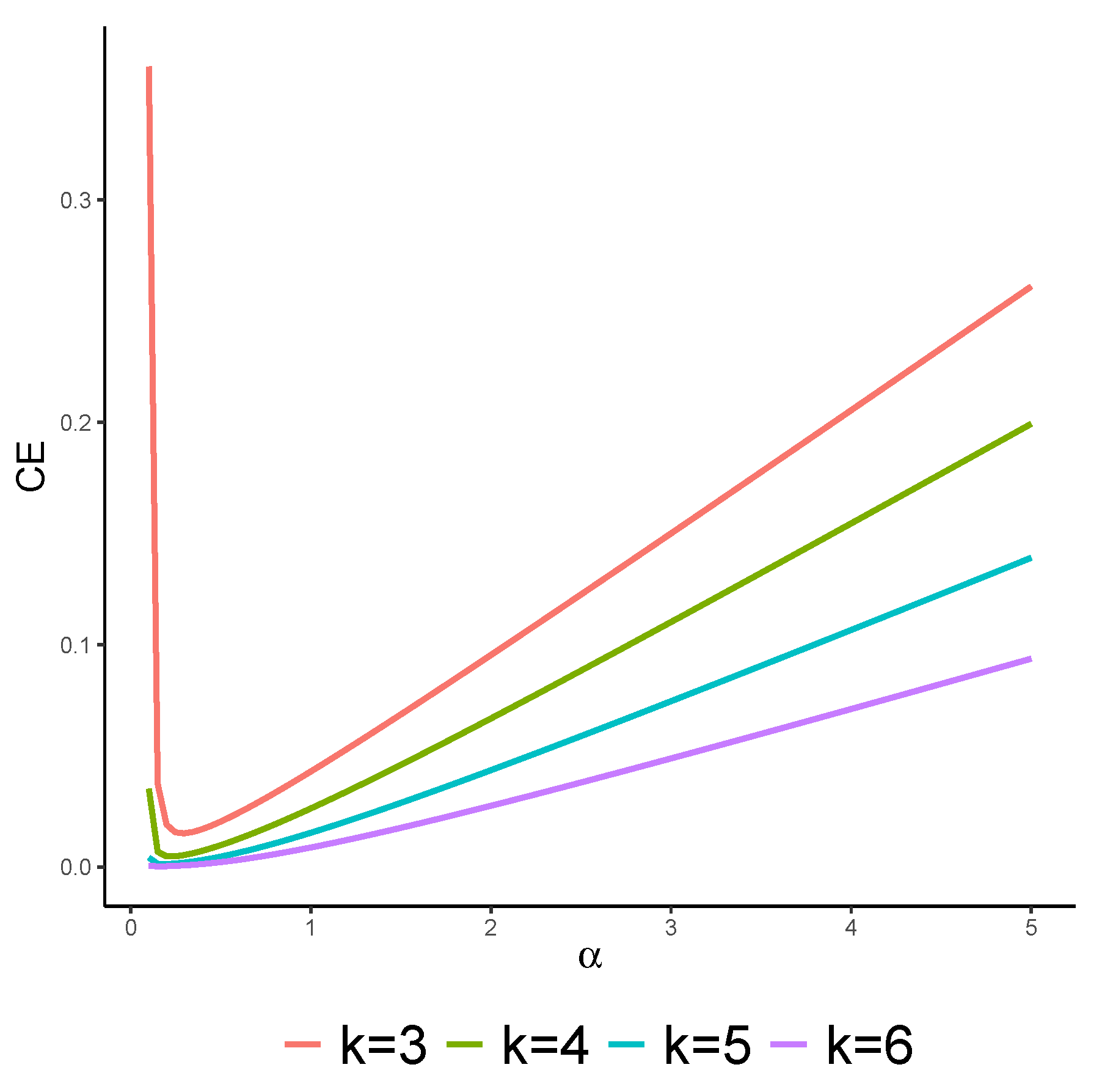

Table 1.
The Bias and RMSE of the first estimator for different choices of k and
| n | k | Bias | RMSE | Bias | RMSE | Bias | RMSE | Bias | RMSE | Bias | RMSE |
| 5 | 3 | -0.124138 | 0.230344 | -0.100742 | 0.191860 | -0.095708 | 0.171305 | -0.093843 | 0.160603 | -0.094036 | 0.131869 |
| 4 | -0.038756 | 0.263316 | 0.000577 | 0.231150 | 0.036344 | 0.218155 | 0.051543 | 0.201405 | 0.093028 | 0.173277 | |
| 5 | -0.091323 | 0.287947 | -0.009914 | 0.253112 | 0.038630 | 0.247169 | 0.066143 | 0.237489 | 0.147523 | 0.237116 | |
| 6 | 3 | 0.072069 | 0.167615 | 0.070267 | 0.138012 | 0.066130 | 0.124728 | 0.061647 | 0.109277 | 0.040760 | 0.075014 |
| 4 | -0.031567 | 0.239911 | 0.010755 | 0.209871 | 0.022254 | 0.184367 | 0.035022 | 0.174554 | 0.055193 | 0.134261 | |
| 5 | -0.151385 | 0.310038 | -0.079245 | 0.260249 | -0.048472 | 0.232668 | -0.015527 | 0.219851 | 0.041610 | 0.175196 | |
| 6 | -0.272339 | 0.380990 | -0.184579 | 0.315350 | -0.127539 | 0.277684 | -0.088733 | 0.253952 | 0.009005 | 0.199077 | |
| 7 | 4 | 0.021823 | 0.208960 | 0.042960 | 0.183286 | 0.054940 | 0.161538 | 0.054626 | 0.150306 | 0.057243 | 0.113776 |
| 5 | -0.092157 | 0.269532 | -0.034616 | 0.238141 | -0.008311 | 0.214772 | 0.008427 | 0.198731 | 0.051931 | 0.159579 | |
| 6 | -0.213470 | 0.350137 | -0.135670 | 0.289292 | -0.086826 | 0.260511 | -0.055488 | 0.242480 | 0.031440 | 0.186683 | |
| 7 | -0.331163 | 0.417481 | -0.230386 | 0.349043 | -0.161969 | 0.305570 | -0.130153 | 0.279632 | -0.007831 | 0.216406 | |
| 8 | 4 | 0.075346 | 0.191621 | 0.080118 | 0.161910 | 0.074436 | 0.143996 | 0.076248 | 0.134626 | 0.059875 | 0.092973 |
| 5 | -0.035972 | 0.244008 | 0.000687 | 0.214961 | 0.023995 | 0.194971 | 0.038143 | 0.183108 | 0.061133 | 0.145446 | |
| 6 | -0.168064 | 0.312048 | -0.088598 | 0.260961 | -0.048191 | 0.238333 | -0.020311 | 0.224606 | 0.037779 | 0.178471 | |
| 7 | -0.291871 | 0.384639 | -0.185520 | 0.314696 | -0.129251 | 0.281766 | -0.093509 | 0.254625 | 0.004763 | 0.198204 | |
| 8 | -0.385751 | 0.455766 | -0.276726 | 0.378007 | -0.211355 | 0.332942 | -0.163147 | 0.300208 | -0.034566 | 0.218227 | |
Table 2.
The Bias and RMSE of the second estimator for different choices of k and
| n | k | Bias | RMSE | Bias | RMSE | Bias | RMSE | Bias | RMSE | Bias | RMSE |
| 5 | 3 | -0.025125 | 0.175512 | -0.014116 | 0.141257 | -0.015236 | 0.123774 | -0.012079 | 0.109911 | -0.005279 | 0.078412 |
| 4 | -0.072958 | 0.267537 | -0.050056 | 0.219368 | -0.029108 | 0.190125 | -0.032334 | 0.172732 | -0.012504 | 0.123541 | |
| 5 | -0.123044 | 0.332033 | -0.084990 | 0.272151 | -0.055920 | 0.239984 | -0.048001 | 0.219015 | -0.023000 | 0.156351 | |
| 6 | 3 | -0.001871 | 0.132976 | 0.000809 | 0.109061 | 0.000794 | 0.092947 | -0.000688 | 0.082732 | -0.000010 | 0.058974 |
| 4 | -0.045391 | 0.228448 | -0.028728 | 0.182676 | -0.024040 | 0.157982 | -0.016516 | 0.145011 | -0.011101 | 0.102678 | |
| 5 | -0.100189 | 0.299852 | -0.064542 | 0.250162 | -0.049838 | 0.217331 | -0.038395 | 0.195598 | -0.018189 | 0.139785 | |
| 6 | -0.131134 | 0.357338 | -0.099022 | 0.297588 | -0.077961 | 0.262055 | -0.057160 | 0.238616 | -0.028988 | 0.170018 | |
| 7 | 4 | -0.026347 | 0.182529 | -0.018355 | 0.150178 | -0.011043 | 0.133090 | -0.010400 | 0.117107 | -0.006821 | 0.083850 |
| 5 | -0.075611 | 0.266131 | -0.041516 | 0.221699 | -0.037394 | 0.192767 | -0.029404 | 0.171981 | -0.014986 | 0.122495 | |
| 6 | -0.124722 | 0.331439 | -0.081209 | 0.278495 | -0.064191 | 0.245961 | -0.050115 | 0.219265 | -0.026817 | 0.155459 | |
| 7 | -0.169382 | 0.377862 | -0.106689 | 0.319331 | -0.086256 | 0.286752 | -0.068001 | 0.256148 | -0.032641 | 0.182052 | |
| 8 | 4 | -0.002768 | 0.152239 | -0.003317 | 0.119965 | 0.000883 | 0.106233 | 0.001972 | 0.094212 | -0.000304 | 0.066692 |
| 5 | -0.052062 | 0.233434 | -0.032683 | 0.190547 | -0.027234 | 0.163031 | -0.021617 | 0.147743 | -0.008801 | 0.104927 | |
| 6 | -0.096677 | 0.298313 | -0.065127 | 0.255635 | -0.048338 | 0.221591 | -0.041602 | 0.196996 | -0.019996 | 0.140928 | |
| 7 | -0.141255 | 0.362541 | -0.094531 | 0.302222 | -0.081784 | 0.265432 | -0.062192 | 0.240006 | -0.026913 | 0.168080 | |
| 8 | -0.181689 | 0.401899 | -0.131193 | 0.343492 | -0.091136 | 0.300505 | -0.070395 | 0.267088 | -0.035192 | 0.200356 | |
Table 3.
Comparison of theoretical values and estimates of CE of based on Weibull distribution for active repair times (in hours) for an airborne communication transceiver.
Table 3.
Comparison of theoretical values and estimates of CE of based on Weibull distribution for active repair times (in hours) for an airborne communication transceiver.
| k | ||||||
|---|---|---|---|---|---|---|
| 3 | 0.188772 | 3.202371 | 2.708464 | 0.139103 | 2.307699 | 1.786721 |
| 4 | 0.252975 | 4.412466 | 4.098577 | 0.225504 | 3.978375 | 3.511787 |
| 5 | 0.282173 | 4.786405 | 4.902895 | 0.267998 | 4.650849 | 4.532230 |
| 6 | 0.289143 | 4.779245 | 5.167557 | |||
| k | ||||||
| 4 | 0.191428 | 3.414607 | 2.827453 | 0.151613 | 2.737446 | 2.057078 |
| 5 | 0.247997 | 4.397852 | 4.073618 | 0.223027 | 4.043979 | 3.538539 |
| 6 | 0.278365 | 4.738680 | 4.867858 | 0.263090 | 4.605239 | 4.497665 |
| 7 | 0.294482 | 4.708580 | 5.384117 | 0.285978 | 4.731164 | 5.137700 |
| 8 | 0.298730 | 4.597261 | 5.563095 |
Disclaimer/Publisher’s Note: The statements, opinions and data contained in all publications are solely those of the individual author(s) and contributor(s) and not of MDPI and/or the editor(s). MDPI and/or the editor(s) disclaim responsibility for any injury to people or property resulting from any ideas, methods, instructions or products referred to in the content. |
© 2024 by the authors. Licensee MDPI, Basel, Switzerland. This article is an open access article distributed under the terms and conditions of the Creative Commons Attribution (CC BY) license (http://creativecommons.org/licenses/by/4.0/).
Copyright: This open access article is published under a Creative Commons CC BY 4.0 license, which permit the free download, distribution, and reuse, provided that the author and preprint are cited in any reuse.


