
Submitted:
28 January 2025
Posted:
28 January 2025
You are already at the latest version
Abstract
This paper introduces novel classes of lifetime distributions characterized by the ratio of failure rate and reversed failure rate functions, evaluated at two distinct points. These classes extend existing stochastic reliability models by incorporating detailed relative aging behaviors, offering a robust framework for analyzing system aging, performance degradation, and failure dynamics under uncertainty. The preservation properties of these classes under order statistics are rigorously analyzed, providing insights into their relationships with established reliability measures. Applications of these findings in predictive maintenance, failure forecasting, and reliability optimization demonstrate their relevance to operational decision-making. By addressing the complexities of aging phenomena and variability in system performance, this study contributes to the advancement of stochastic modeling in reliability engineering and provides practical tools for tackling modern challenges in critical industries such as aerospace, manufacturing, and infrastructure.
Keywords:
Failure rate
; Reversed failure rate
; Relative aging
; IFR
; Order statistics
MSC: 60K10; 90B25
1. Introduction
In reliability modeling and survival analysis, lifetime distributions are fundamental tools for analyzing the stochastic behavior of time-to-failure in systems and components. These distributions provide critical insights into system reliability, aging phenomena, and performance degradation under uncertainty. Designed to accommodate non-negative data, they have broad applications in operational and engineering contexts, ranging from predictive maintenance to failure forecasting. Over time, several non-parametric classes of lifetime distributions have been developed, each characterized by unique properties to model specific aspects of aging. In reliability theory, aging refers to the progressive increase in failure probability as a system ages, contrasting with systems that exhibit constant failure rates, where aging is absent. The distinction between a system’s calendar age and its performance as it ages is critical for evaluating reliability. A failure in this context is defined as the termination of a necessary function, while reliability refers to the system’s ability to perform its intended operations within specified standards.
The survival function (sf) or reliability function, denoted as , represents the probability that a system will successfully operate without failure up to time x. It characterizes the lifetime distribution of the system. Specifically, the probability that the failure time (a random variable X) occurs after time is given by the sf evaluated at x. From a novel perspective, new reliability concepts can be introduced to describe the aging phenomenon in living organisms more effectively. Several life distribution classes have been proposed to model aging in greater detail. The rate of aging is commonly described in reliability theory and survival analysis through the failure rate (FR) function. This function measures the instantaneous risk of failure at a given point in time, conditional on the system or component surviving up to that point. The FR function for a random variable X (which represents the time to failure) is defined as follows:
where is the pdf of the rv . The FR represents the current risk of failure at time . A higher value of indicates a greater probability of failure at that moment. In the context of earthquake engineering, probabilistic seismic hazard analysis, an area that has attracted significant attention from researchers, utilizes for analytical evaluation. There is also a similar method that uses the reversed failure rate (RFR) function , where is the cumulative distribution function of . This measure is widely used to classify lifetime distributions (Barlow and Proschan (1996), Klein and Moeschberger (2006), Marshall and Olkin (2007), Rehman et al. (2018), Khan et al. (2020), Rahman et al. (2021) and Ahmed et al. (2022)).
The speed of aging is a novel aspect of life distribution that can be interpreted as how quickly the FR increases over time. The speed of aging in terms of the FR function reflects how fast the risk of failure increases (or decreases) over time. This relationship is critical to understanding the reliability and lifetime of systems and components and allows for better maintenance planning and risk management strategies. This can be quantified by analyzing the derivative of the FR function. The speed of aging can be assessed by examining the derivative as follows:
- If , then the aging speed is positive, indicating that the system's risk of failure is increasing over time.
- , then the aging speed is negative, suggesting that the risk of failure is decreasing.
- , then the aging has a constant speed.
In reliability engineering, the behavior of the FR function over time provides critical insights into the aging characteristics of a system or component. For example, service life distributions are typically categorized into three classes based on the behavior of the FR function:
- Increasing Failure Rate (IFR): If is increasing, it implies that the system is becoming more prone to failure as time progresses. This is characteristic of "aging" systems where wear and tear accumulate over time.
- Decreasing Failure Rate (DFR): If is decreasing, it suggests that the system is becoming less likely to fail as time goes on, which can occur in certain contexts like burn-in periods.
- Constant Failure Rate (CFR): If is constant, it indicates that failures occur uniformly over time, typical of systems with no aging effects, such as in exponential distributions.
Probability distributions play a crucial role in reliability engineering, offering robust methodologies for modeling various types of reliability data and underlying failure mechanisms. Selecting an appropriate distribution is paramount, as it directly affects the accuracy of operational decision-making. This choice should be guided by empirical data and theoretical considerations. Distributions with IFR properties are particularly valuable for modeling the lifetimes of products and components in industries such as mechanics, electronics, and materials science, where aging and wear significantly impact reliability. Identifying IFR behavior has important implications for reliability analysis, including optimizing maintenance schedules, improving warranty strategies, and mitigating risk. Systems exhibiting IFR characteristics often necessitate more frequent inspections or proactive maintenance to prevent unexpected failures. Recognizing whether a system falls into the IFR category provides essential insights for optimizing maintenance practices and ensuring operational reliability in the long term (Lai and Xie (2006), Finkelstein (2008), and Navarro (2022)).
This paper introduces new classes of lifetime distributions, characterized by a nuanced and dynamic behavior of the failure rate (FR) function. These classes extend beyond the traditional emphasis on monotonicity (whether the FR is increasing or decreasing) to capture variations in the intensity of FR ratios over time, providing a richer and more detailed framework for analyzing aging processes. By exploring relationships among these proposed classes, we establish necessary and sufficient conditions for a random variable to belong to each class. Additionally, the preservation properties of these novel life distribution classes under order statistics are rigorously analyzed, offering insights into their applicability in stochastic modeling and reliability analysis.
The remainder of this paper is structured as follows. Section 2 introduces the definitions, descriptions, and preliminary properties of the proposed life distribution classes, with a focus on the aging speed phenomenon and relative aging concepts, which are central to stochastic reliability analysis. Section 3 explores the preservation properties of these classes under various structural frameworks, including order statistics and related reliability models, providing insights into their robustness and practical utility. Section 4 presents practical applications of the findings, emphasizing their relevance to predictive maintenance, reliability optimization, and operational decision-making in engineering systems. Finally, Section 5 concludes by summarizing the key contributions and outlining potential directions for future research, particularly in stochastic modeling and complex system reliability analysis.
2. Some Novel Life Distribution Classes
This section introduces the definitions, descriptions, and preliminary properties of novel classes of life distributions that incorporate the aging speed phenomenon, a key aspect in stochastic reliability analysis. The concept of relative aging is employed to establish an order relation between two lifetime distributions, facilitating comparisons of aging rates across different units. This framework extends naturally to describe the aging behavior of individual lifetime units, enabling a more granular understanding of system reliability. The following definition serves as the foundation for the development of these novel classes.
Definition 2.1.
Let be a non-negative with function and function . Then, it is said that has:
- (i).
- increasing (decreasing) failure rate ratio property [denoted by , whenever is increasing (decreasing) in , for all .
- (ii).
- increasing (decreasing) reversed failure rate property [denoted by , whenever is increasing (decreasing) in , for all .
- (iii).
- increasing (decreasing) failure rate relative to average failure rate property [denoted as ( , whenever is increasing (decreasing) in (Righter et al. (2009)).
- (iv).
- increasing (decreasing) reversed failure rate relative to average reversed failure rate property [denoted as , whenever is increasing (decreasing) in .
Table 1 provides a summary of parametric families of lifetime distributions exhibiting the IFRR and DFRR properties. In contrast, Table 2 presents examples of lifetime distributions belonging to the IRFRR and DRFRR classes.
Remark 2.1.
It is noteworthy that the classes defined in (iii) and (iv) are closely associated with the concepts of the aging intensity (AI) function and the reversed aging intensity (RAI) function, respectively. Let be a non-negative rv with sf and hr function , then is called the AI function of . In this case is equivalent to saying that has an increasing (a decreasing) AI function. If has cdf and rhr function , then is called the RAI function of (see, for instance, Kayid and Alshehri (2024)). In this setting, ( ) holds if, and only if, has an increasing (a decreasing) RAI function.
The relationships between the life distribution classes introduced in Definition 2.1 are established as follows.
Proposition 2.3.
The following implications hold:
- (i).
- .
- (ii).
- .
Proof.
Part (i). Suppose has function . From Remark 2.1, it is sufficient to show that is an increasing [a decreasing] function. We have
where the last expression is due to the change of variable . Now, assume that . Then, according to Definition 2.1(i), is decreasing [increasing] in , for all . Thus, is also decreasing [increasing] in .
Part (ii). Let have function . As clarified in Remark 2.2, we need only to show is an increasing [a decreasing] function. We get
Suppose that . Then, from Definition 2.1(ii), is decreasing [increasing] in , for all . Hence, is increasing [decreasing] in , for all . As a result, is increasing [decreasing] in . The required result is obtained.
The following proposition presents a necessary and sufficient condition under which ) and also presents another similar necessary and sufficient condition under which holds.
Proposition 2.4.
Let and be two differentiable functions.
- (i).
- if, and only if, is increasing (decreasing) in .
- (ii).
- if, and only if, is increasing (decreasing) in .
The following example illustrates a distribution with a non-monotonic failure rate function that belongs to the DFRR class.
Example 2.5.
The random variable is said to have the DRFR property if its reversed failure rate function is a decreasing function.
Proposition 2.6.
- (i).
- If is increasing (i.e. if is IFR) and also log-convex in , then .
- (ii).
- If is decreasing (i.e. if is DFR) and log-concave in , then .
- (iii).
- If is decreasing (i.e. if is DRFR) and log-concave, then .
Proof.
Denote . To prove (i), note that if is increasing and log-convex, then is non-negative and increasing in . Thus, is also increasing in . From Proportion 2.4(i), we deduce that .
The following example presents an application of Proposition 2.6(i) in a specific model.
Example 2.7.
Let be uniformly distributed on where . We have where . So, is IFR. We can see that which is increasing in . Therefore, is log-convex in . Using Proposition 2.6(i), is IFRR.
3. Preservation of and Classes
3.1. Extreme Order Statistics
We consider order statistic , when and . Since , for all , thus , for all . Therefore, , for all and for all . According to Definition 2.1(i), this means that is IFRR (DFRR) if, and only if, is IFRR (DFRR). On the other hand, since , for all , thus , for all . As a result, , for all and for all . By Definition 2.1(ii), this is equivalent to saying that is IFRRR (DRFRR) if, and only if, is IRFRR (DRFRR). However, for , the preservation properties of the DFRR and DRFRR classes under the structure of order statistics are as we discuss in the next subsection.
3.2. Order Statistics
In this subsection, we present and rigorously prove the preservation properties of the class and the class under order statistics. Let and be two non-negative random variables with respective sf’s and and also respective density functions and . Then, it is said that is smaller (bigger) than in the usual stochastic order (denoted by ) if , for all . Equivalently, if for all increasing functions or for all decreasing functions where all expectations are assumed to exist and are finite. Furthermore, it is said that is smaller (bigger) than in the likelihood ratio order (denoted by ) whenever is increasing (decreasing) in . From Shaked and Shanthikumar (2007), (resp. ) implies that (resp. ). Before stating the main results of this subsection, we state a useful technical lemma.
Lemma 3.1.
Let for , where . Then is increasing in .
Proof.
We see that
Therefore,
For all one has
By substituting form the above expression in the numerator of the second ratio in last line of Equation (1), we obtain
where
Hence, as a result,
and it is enough to show that
is a non-negative increasing function because is non-negative and increasing in from Example 5 in Kayid and Almohsen (2024). Since is increasing in for all , thus in the spirit of is non-negative for all . Now, we show that is increasing in . Notice that from (3), where is a non-negative random variable with pdf
It is straightforward to see that is increasing in , for all . That is , for all . Since likelihood ratio order implies the usual stochastic order, thus we further conclude that , for all . Now, since is decreasing function in , thus, by definition we have , for all , i.e. is increasing in .
In this section, we assume that are independent and identically distributed (i.i.d.) random variables with common sf , and pdf . The first result of this section is as follows:
Theorem 3.2.
implies that where .
Proof.
It can be seen that the failure rate function of is derived as
We need to prove that is decreasing in , for all . From Equation (4), we have
Since , thus is decreasing in , for all . Therefore, and the proof obtains if we show in addition that
is also decreasing in , for all where for every . To this end, we show that , for all , and for all . From the parenthetical part of Proposition 2.3(i), since , thus . As a result,
It is not hard to prove that is increasing in which further implies that , for all , and further , for all . By multiplying both sides of (6) in , for all , and for all we derive
For all , we get
where
and the inequality is due to (7). It is notable that and as a result , for all . Therefore, is non-positive if, and only if,
Since , for all and for all , from which one gets , for all . Let us define which by Lemma 3.1 it is a decreasing function in . The inequality given in (9) can be written accordingly as , for all . The proof of the theorem is now complete.
The following example illustrates a practical scenario to validate and examine the correctness of the result established in Theorem 3.2.
Example 3.3.
Let be non-negative i.i.d random variables with sf 0. Note that , which is a decreasing function in . From the parenthetical part of Proposition 2.4(i), is DFRR. Consider the second order statistic and note that
from which one gets
Figure 3 exhibits the graph of the function which is seen to be decreasing in . This acknowledges from the parenthetical part of Proposition 2.4 that is DFRR.
The next result establishes the preservation of the DRFRR class under the formation of order statistics.
Theorem 3.4.
If , then for .
Proof.
The reversed failure rate functions of is obtained as
We have to prove that is decreasing in , for all . It is seen from Equation (10) that
As , thus is decreasing in , for all . Note that is defined as in the proof of Theorem 3.2. In view of (11), and the proof is completed if we demonstrate that
is decreasing in , for all . To prove this, we show that , for all , and for all . By the parenthetical part of Proposition 2.3(ii), since , thus . Thus,
For simplicity we write , for all . Since is increasing in which also gives , for all , and furthermore , for all . By multiplying both sides of (12) in , for all , it is deduced that
Next, for all , one has
where
and the inequality follows from (13). Note that for all . Thus, is non-positive for all if, and only if, for all and for all it holds that
Notice that , for all and for every , which implies that . Define which by Lemma 3.1 it is a decreasing function in . It can be seen that the inequality given in (15) holds if, and only if, , for all and for every which holds true because is a decreasing function. The proof follows immediately.
The next example demonstrates a practical scenario that highlights the applicability of Theorem 3.4.
Example 3.5.
Suppose that are non-negative i.i.d random variables with cumulative distribution function . It can be seen that , which is decreasing in . By using the parenthetical part of Proposition 2.4(ii), is DRFRR. Note that
Therefore,
In Figure 4 the curve of the graph of the function is plotted for which exhibits a decreasing behaviour. From the parenthetical part of Proposition 2.4(ii), this confirms that that is DRFRR.
4. Illustrations and Remarks
The results obtained in this paper have several potential applications. For instance, Proposition 2.4 provides a practical approach to estimating future values of the failure rate (or reversed failure rate) function for a lifetime unit based on its current values. However, applying this approach requires careful consideration of the underlying statistical model and the assumptions about the data to ensure validity. The properties of IFRR (DFRR) and IRFRR (DRFRR), play a crucial role in this estimation process. These properties allow for the development of recursive formulas for both the failure rate and reversed failure rate functions. To illustrate this, we explain how this idea emerges for a random variable exhibiting the IFRR property.
Let be the random lifetime of a unit with IFRR property. Then, according to Proposition 2.4(i), is increasing function in and vice versa. Suppose that is IFRR and that the amount of is known at time point . Then, from Proposition 2.4(i), there exists an increasing function such that for all . The same explanations can be given for the case when lies in one of the DFRR, IRFRR classes or the DRFRR class. From the perspective of regression theory, it is valuable to estimate the failure rate function (or reversed failure rate function) at a future time point based on its value at a current time. Estimating a future failure rate function (or reversed failure rate function) based on an already known value is possible if the random variable which is under consideration, has one of the IFRR, DFRR, IRFRR or DRFRR properties. These properties provide a foundation for developing predictive models that extend the reliability analysis into future time points. In this section, we perform a simulation study to evaluate the performance of a linear regression model within the framework of a lifetime distribution exhibiting the IFRR property.
From Table is said to have Gompertz distribution with parameters and if it has sf . The associate failure rate function is given by . It can then be seen that where .
We generate 36 samples from Gompertz distribution with parameters and by using the inverse transform technique. Specifically, by applying the function runif in R, we generate uniform random variables on [0,1. Then, using the inverse transform technique with , for and one gets:
by which one can generate a random sample of size 36 from the Gompertz distribution with and . In addition, we also calculate with and generate such that 's are i.i.d. with standard normal distribution with variance 0.01. Then we obtain with and .
Let us consider the simple regression model where represents random error terms. Using the method of least squares, we estimate the parameter . The simulated data in R yield an estimate of . Table 3 presents the simulated data alongside the corresponding values of the failure rate ratio
The results of Theorem 3.2 and Theorem 3.4 can be utilized to establish preservation properties of DFRR and DRFRR classes under the structure of -out-of- systems in reliability analysis as the lifetime of such systems are represented by order statistics.
Let denote the lifetimes of components of a -out-of system, then the lifetime of the whole system is which is the ()th smallest value among . In general, the -out-of- systems provide a common model in reliability engineering, where a system is considered functional if at least out of components are operational. In aviation in aircraft systems, certain critical systems like flight control might be designed as a 2 -out-of- 3 system.
For instance, if there are three independent flight control computers, the aircraft can still operate safely as long as two of them are functioning. This redundancy is crucial for safety and reliability in flight operations. In the context of railway signaling systems, a system might utilize a 2-out-of-4 architecture where multiple signal lights must be operational to indicate safe passage for trains. This design minimizes the risk of signaling errors that could lead to accidents. In these scenarios, if the time-to-failure distributions of individual components belong to the DFRR or DRFRR classes, the time-to-failure of the entire system will also have a distribution that belongs to the same class. This highlights the importance of these reliability classes in modeling and analyzing the performance of redundant systems.
5. Conclusions
This study introduces the IFRR (DFRR) and IRFRR (DRFRR) classes of lifetime distributions, emphasizing the relative behavior of the failure rate and reversed failure rate at two distinct points. By analyzing the monotonicity and variation of these rates, we provide a comprehensive framework for characterizing aging phenomena in reliability systems. The derived conditions and preservation properties under order statistics demonstrate the versatility and practical applicability of these classes in modeling real-world reliability challenges. The monotonicity of the failure rate (or reversed failure rate) relative to its value at a previous time was thoroughly analyzed. For instance, a lifetime distribution possessing the IFR and IFRR properties indicates that the failure rate increases more rapidly over time, while a distribution with the IFR and DFRR properties implies that the rate of increase of the failure rate diminishes over time. These analyses establish a strong connection between the proposed classes and monotone classes defined by aging intensity and reversed aging intensity functions (see Proposition 2.3).
To illustrate the applicability of these classes, Table 1 and Table 2 summarize several distributions that belong to the IFRR (DFRR) and IRFRR (DRFRR) classes. Proposition 2.4 establishes necessary and sufficient conditions for a lifetime distribution to possess the IFRR/DFRR (or IRFRR/DRFRR) property. Additionally, Proposition 2.6 extends this by providing conditions for distributions with IFR/DFR properties to also exhibit the IFRR/DFRR (or DRFRR) property. Preservation properties of the DFRR and DRFRR classes under order statistics were rigorously derived (Theorems 3.2 and 3.4), further highlighting the robustness of these models.
Future research will explore additional applications of the proposed classes, particularly in record statistics, such as upper records, k-records, and lower records. Investigating whether these classes are preserved under such models will extend their utility in reliability and complex system analysis.
Acknowledgments
This work was supported by Researchers Supporting Project number (RSP2025R392), King Saud University, Riyadh, Saudi Arabia.
References
- Ahmed, M., Lodi, S.H. and Rafi, M.M. (2022). Probabilistic seismic hazard analysis-based zoning map of Pakistan. Journal of Earthquake Engineering, 26(1), 271-306.
- Barlow, R.E. and Proschan, F. (1996). Mathematical theory of reliability. Society for Industrial and Applied Mathematics.
- Elgohari, H., Ibrahim, M., Yousof, H.M. (2021). A new probability distribution for modeling failure and service times: properties, copulas and various estimation methods. Statistics, Optimization and Information Computing, 9(3), 555-586.
- Finkelstein, M. (2008). Failure Rate Modelling for Reliability and Risk. Springer Science and Business Media.
- Gavrilov, L.A. and Gavrilova, N.S. (2005). Reliability Theory of Aging and Longevity. Handbook of the Biology of Aging, 3-42.
- Jiang, R., Ji, P. and Xiao, X. (2003). Aging property of unimodal failure rate models. Reliability Engineering and System Safety, 79(1), 113-116.
- Kayid, M., and Alshehri, M.A. (2024). Stochastic aspects of reversed aging intensity function of random quantiles. Journal of Inequalities and Applications, 2024(1), 119.
- Kayid, M. and Almohsen, R. A. (2024). Preservation of relative failure rate and relative reversed failure rate orders by distorted distributions. Acta Applicandae Mathematicae, 194(1), 1-15.
- Khan, M.Y., Iqbal, T., Iqbal, T., and Shah, M.A. (2020). Probabilistic modeling of earthquake Interevent times in different regions of Pakistan. Pure and Applied Geophysics, 177(12), 5673-5694.
- Klein, J.P. and Moeschberger, M.L. (2006). Survival Analysis: Techniques for Censored and Truncated Data. Springer Science and Business Media.
- Lai, C.D., and Xie, M. (2006). Stochastic ageing and dependence for reliability. Springer Science and Business Media.
- Marshall, A.W. and Olkin, I. (2007). Life Distributions (Vol. 13). Springer, New York.
- Navarro, J. (2022). Aging Properties. In: Introduction to System Reliability Theory. Springer, Cham.
- Rehman, K., Burton, P.W. and Weatherill, G. A. (2018). Application of Gumbel I and Monte Carlo methods to assess seismic hazard in and around Pakistan. Journal of Seismology, 22, 575-588.
- Rahman, A.U., Najam, F.A., Zaman, S., Rasheed, A. and Rana, I.A. (2021). An updated probabilistic seismic hazard assessment (PSHA) for Pakistan. Bulletin of Earthquake Engineering, 19, 1625-1662.
- Righter, R., Shaked, M. and Shanthikumar, J. G. (2009). Intrinsic aging and classes of nonparametric distributions. Probability in the Engineering and Informational Sciences, 23(4), 563-582.
- Shaked, M. and Shanthikumar, J. G. (Eds.). (2007). Stochastic Orders. New York, Springer, New York.
Figure 1.
Plot of the function for in Example 2.5.
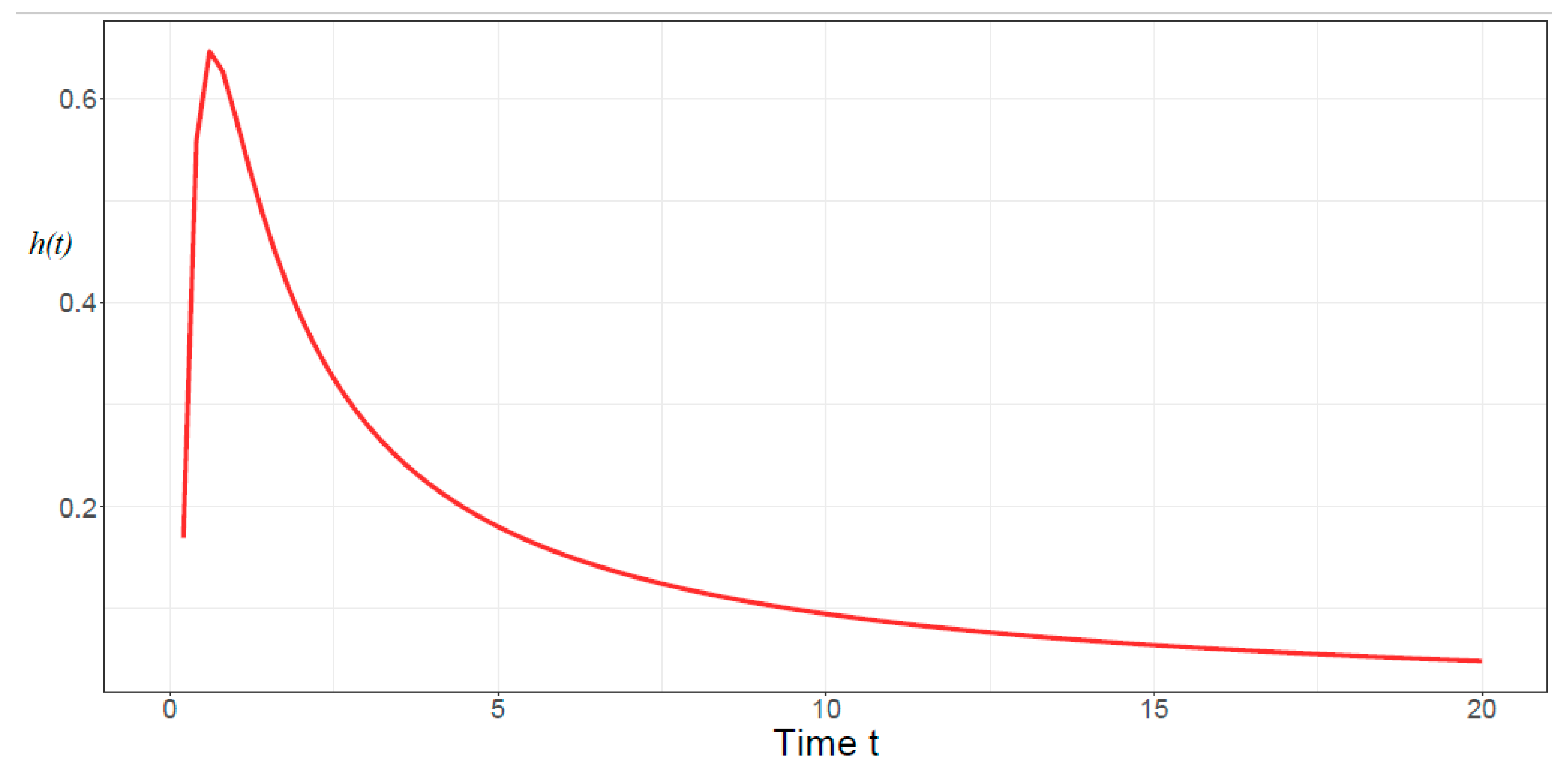
Figure 2.
Plot of the function for in Example 2.5.
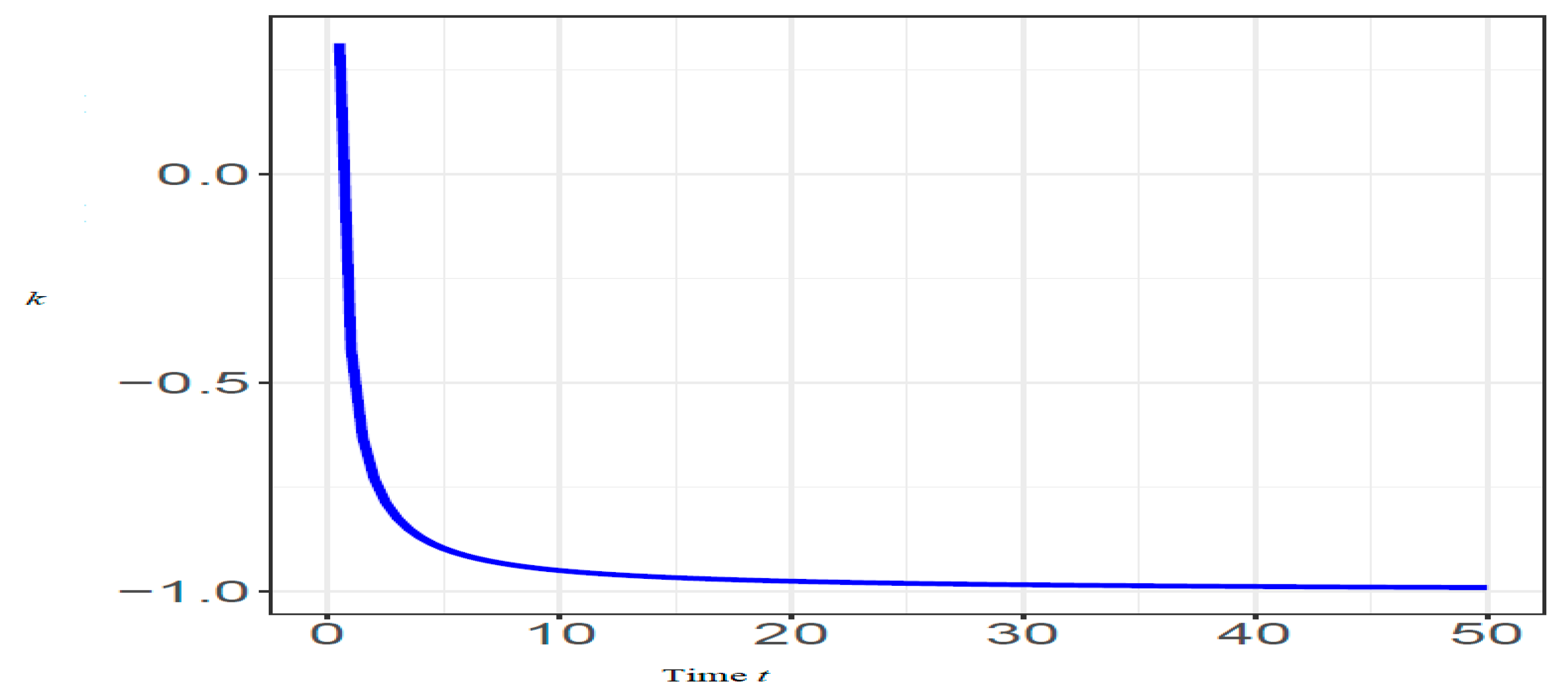
Figure 3.
Plot of the function for in Example 3.3.
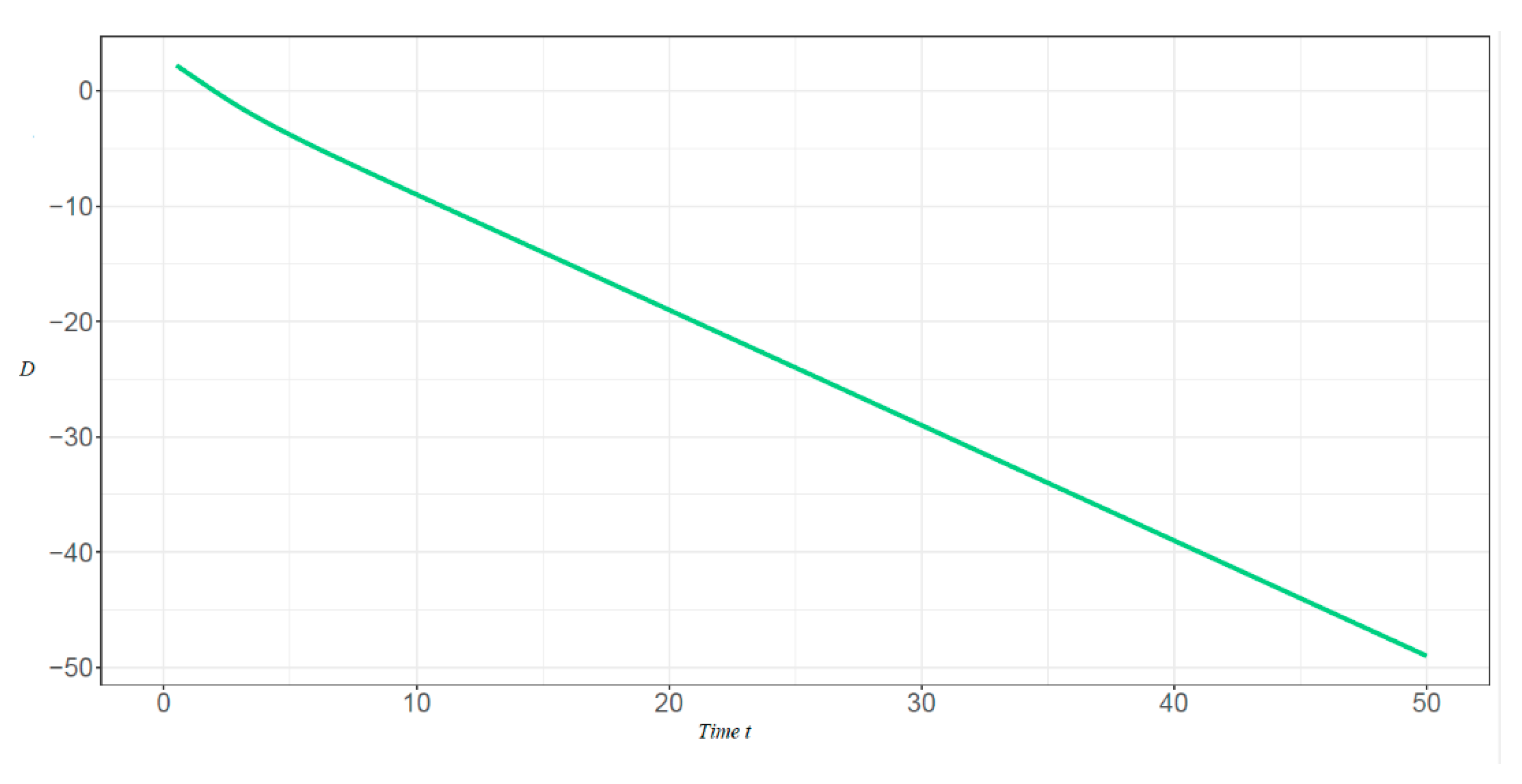
Figure 4.
Plot of the function for in Example 3.5 the random lifetime.
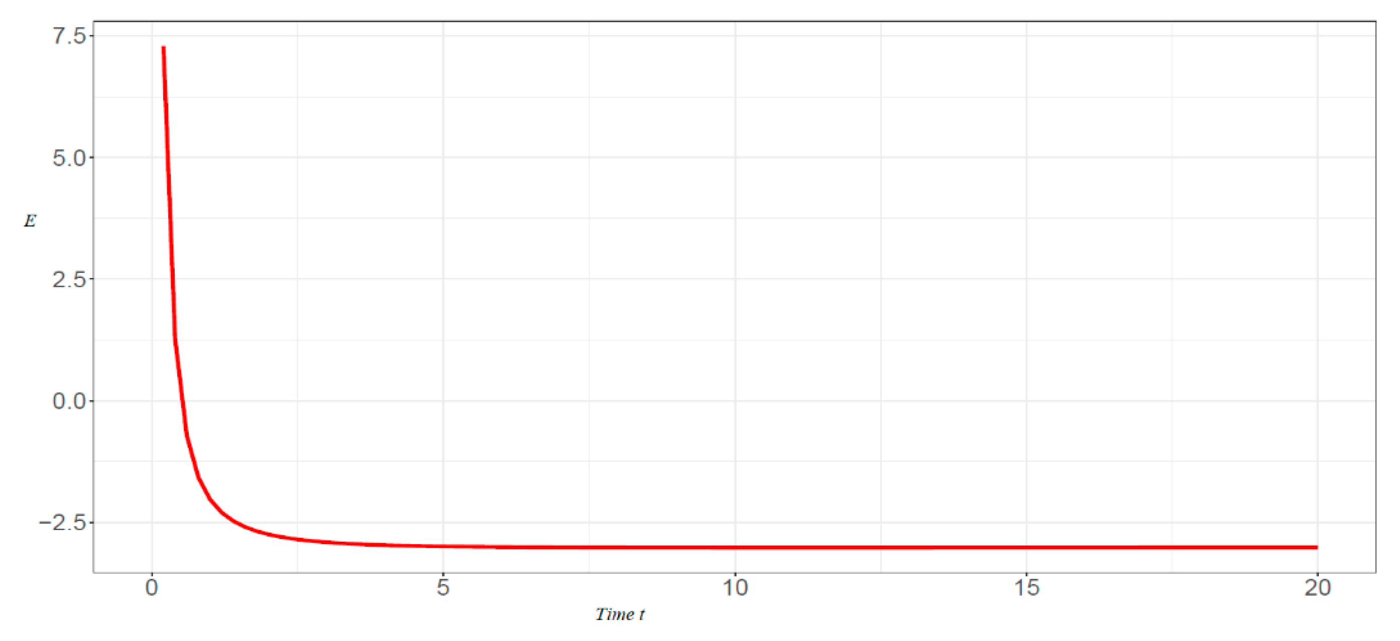

Table 1.
Some distributions with their classes of life distributions.
| Distribution | Survival function | Failure rate | Classes of life distributions |
| IFRR, DFRR | |||
| IFRR | |||
| IFRR, DFRR | |||
| DFRR | |||
| DFRR | |||
| , | DFRR | ||
| , | IFRR | ||
| IFRR |
Table 2.
Table of some other distributions with their classes of life distribution.
| Distribution | Distribution function | Reversed failure rate | Classes of life distributions |
| Uniform | IRFRR, DRFRR | ||
| IRFRR, DRFRR | |||
| IRFRR, DRFRR | |||
| DRFRR | |||
| a | IRFRR, DRFRR | ||
| Reversed generalized Pareto |
IRFRR (1 < a < 0), DRFRR (a > 0) |
||
| Half-logistic | , | DRFRR | |
| , | IRFRR |
Table 3.
The data and the collected values.
| 0.4994765579 | 0.665968438 | 0.663175700 | 0.3767697318 | 0.5023596424 | 0.481206988 |
| 0.0262070426 | 0.0349427235 | 0.044638045 | 0.2760793150 | 0.3681057533 | 0.379140003 |
| 0.4268042135 | 0.5690722846 | 0.552286801 | 0.1202760829 | 0.1603681105 | 0.153914794 |
| 0.6347501182 | 0.8463334910 | 0.856256977 | 0.6925388390 | 0.9233851187 | 0.913135678 |
| 0.1062242823 | 0.1416323764 | 0.149734467 | 0.4858971732 | 0.6478628975 | 0.649624370 |
| 0.0020145895 | 0.0026861193 | 0.003775633 | 0.1023574924 | 0.1364766565 | 0.129376481 |
| 0.2021058905 | 0.2694745207 | 0.275697108 | 0.0247524753 | 0.0330033004 | 0.025111582 |
| 0.1250653974 | 0.1667538632 | 0.172243974 | 0.3492021468 | 0.4656028624 | 0.460156151 |
| 0.7632430504 | 1.0176574005 | 0.989129083 | 0.3888029720 | 0.5184039626 | 0.515212907 |
| 0.3313270349 | 0.4417693799 | 0.443656742 | 0.0023579842 | 0.0031439790 | 0.009198710 |
| 0.1914079065 | 0.2552105420 | 0.273083995 | 0.2420603688 | 0.3227471584 | 0.314663449 |
| 0.0222195438 | 0.0296260584 | 0.024211896 | 0.2495684549 | 0.3327579398 | 0.321895450 |
| 0.2309642881 | 0.3079523841 | 0.294108814 | 0.2897415880 | 0.3863221174 | 0.390603567 |
| 0.1388329777 | 0.1851106370 | 0.194475793 | 0.3238376461 | 0.4317835281 | 0.440572804 |
| 0.3314107170 | 0.4418809560 | 0.466452456 | 0.0854768423 | 0.1139691230 | 0.127169177 |
| 0.6436907800 | 0.8582543733 | 0.883448724 | 0.1384879074 | 0.1846505432 | 0.182986975 |
| 0.5571105993 | 0.7428141324 | 0.742170484 | 0.4533983734 | 0.6045311645 | 0.604828181 |
| 0.2168994877 | 0.2891993169 | 0.272227298 | 0.2409825121 | 0.3213100162 | 0.308286976 |
Disclaimer/Publisher’s Note: The statements, opinions and data contained in all publications are solely those of the individual author(s) and contributor(s) and not of MDPI and/or the editor(s). MDPI and/or the editor(s) disclaim responsibility for any injury to people or property resulting from any ideas, methods, instructions or products referred to in the content. |
© 2025 by the authors. Licensee MDPI, Basel, Switzerland. This article is an open access article distributed under the terms and conditions of the Creative Commons Attribution (CC BY) license (http://creativecommons.org/licenses/by/4.0/).
Copyright: This open access article is published under a Creative Commons CC BY 4.0 license, which permit the free download, distribution, and reuse, provided that the author and preprint are cited in any reuse.


