Submitted:
14 July 2025
Posted:
15 July 2025
You are already at the latest version
Abstract
Object detection in synthetic aperture radar (SAR) imagery poses significant challenges due to low resolution, small objects, arbitrary orientations, and complex backgrounds. Standard object detectors often fail to capture sufficient semantic and geometric cues for such tiny targets. To address this issue, a new Convolutional Neural Network (CNN) framework called Deformable Vectorized Detection Network (DVDNet) has been pro-posed, specifically designed for detecting small, oriented, and densely packed objects in SAR images. The DVDNet consists of Grouped-Deformable Convolution for adaptive receptive field adjustment to diverse object scales, a Local Binary Pattern (LBP) En-hancement Module that enriches texture representations and enhances the visibility of small or camouflaged objects, and a Vector Decomposition Module that enables accurate regression of oriented bounding boxes via learnable geometric vectors. The DVDNet is embedded in a two-stage detection architecture and is particularly effective in preserving fine-grained features critical for small object localization. The performance of DVDNet is validated on two SAR small target detection datasets, HRSID and SSDD, and it is ex-perimentally demonstrated that it achieves 90.9% mAP on HRSID and 87.2% mAP on SSDD. The generalizability of DVDNet was also verified on the remote sensing dataset Pascal VOC 2012 and the generalized dataset HRSC2016. All these experiments show that DVDNet outperforms the standard detector. Notably, our framework shows substantial gains in precision and recall for small object subsets, validating the importance of com-bining deformable sampling, texture enhancement, and vector-based box representation for high-fidelity small object detection in complex SAR scenes.
Keywords:
synthetic aperture radar
; small object
; arbitrary orientations
; grouped-deformable convolution
; local binary pattern
; vector decomposition
1. Introduction
Object detection in SAR images is a crucial task for applications in surveillance, urban planning, traffic monitoring, and disaster management. In recent years, deep learning has led to remarkable advances in generic object detection on natural images [1,2,3,4,5]. Two-stage detectors like Faster R-CNN [2] and one-stage detectors like YOLO [3] achieve high accuracy and speed on benchmarks such as COCO. However, affected by speckle noise, complex imaging geometry and other factors, SAR images present very different characteristics from optical images, and it is often difficult to obtain ideal results by directly migrating the above methods.
There are many challenges in SAR target detection tasks. SAR images typically contain objects at vastly different scales, in arbitrary orientations, in very dense distributions, and against highly complex backgrounds. Standard detectors assume fixed-size receptive fields and mostly axis-aligned bounding boxes, which struggle with these conditions. Small objects may be missed by deep networks optimized for larger objects, rotated objects may not be well enclosed by axis-aligned boxes, densely packed objects can cause overlapping detections to be merged or missed, and background clutter can lead to many false positives. Notably, small object detection remains particularly challenging in SAR scenarios due to limited resolution and scale variance, making it a crucial focus of this work.
Various approaches have been explored to handle individual aspects of these issues. For instance, multi-scale feature pyramids [6] or multi-scale training strategies are used to detect objects of different sizes. For arbitrary orientations, some methods introduce rotated anchors or rotated bounding box regression [7,8,9,10,11] to better localize angled objects. Nevertheless, existing detectors typically address these challenges in isolation and still encounter limitations when faced with the full complexity of SAR imagery. There is a need for a unified approach that can concurrently tackle scale variation, orientation, density, and background clutter [12,13,14,15,16,17].
In this paper, we propose a comprehensive solution, leveraging three key innovations in a single framework. Grouped-Deformable Convolution (GDConv) layers that provide adaptive receptive fields for multi-scale and deformable object shapes while keeping the model efficient. An LBP Enhancement Module that injects rich local texture features (via the classic Local Binary Pattern descriptor) into the CNN feature maps to help distinguish objects from complex backgrounds. A Vector Decomposition Module that predicts each object's bounding box using a pair of vectors, enabling an effective and continuous representation of oriented boxes without angular ambiguities. By integrating these components into a standard CNN-based detection pipeline, our method directly addresses the four challenges described above. GDConv handles scale and shape variation, LBP features improve detection of small or low-contrast objects in clutter, and the vector decomposition handles arbitrary object orientations and aspect ratios. This design is especially beneficial for detecting small targets, which are prevalent and critical in SAR imagery applications.
A novel SAR target detection framework, Deformable Vectorized Detection Network (DVDNet), was designed. It combines grouped deformable convolutions, an LBP-based texture enhancement, and a vector decomposition-based bounding box encoding. To our knowledge, this is the first work to unify these three components in a single detector. In summary, the contributions of this work are as follows.
(1) Grouped Deformable Convolution (GDConv) was designed, which synergistically merges deformable convolution [18] with grouped convolution [19]. This module allows the network to learn adaptive sampling of features while controlling the number of parameters and computational cost.
(2) We design an LBP Enhancement Module that seamlessly integrates Local Binary Pattern computation into the CNN. The module extracts local texture patterns from feature maps and fuses them with learned features, providing complementary cues that improve the detection of small, densely packed objects and reduce false detections in textured backgrounds.
(3) We contrive a Vector Decomposition Module for bounding box regression. Instead of predicting width, height, and orientation angles directly, our detector predicts two vectors from the object’s center to its bounding box sides. This yields a flexible representation for rotated boxes, avoiding issues of angle periodicity and enabling more precise localization of oriented objects.
Finally, we conducted ablation experiments and comparison experiments on two SAR small target detection datasets, HRSID and SSDD, to evaluate the proposed DVDNet. To validate the generalization performance of the model, extensive experiments are also conducted on the general-purpose dataset Pascal VOC 2012 and the remote sensing dataset HRSC2016. DVDNet achieves much higher mAP than the baseline detector on all datasets, with a significant improvement in precision-recall performance. Also, detailed ablation studies and analyses are provided to demonstrate the effectiveness of each proposed component.
The remainder of this paper is organized as follows. Section 2 reviews related work in SAR object detection, deformable/grouped convolutions, and texture/orientation modeling in CNNs. Section 3 presents the proposed method, detailing the overall architecture and each module. Section 4 reports experimental results on four datasets, including quantitative comparisons and discussions. Finally, Section 5 concludes the paper with remarks and future directions.
2. Related Work
2.1. Small Object Detection
Small object detection is one of the most persistent challenges in computer vision, particularly in aerial and remote sensing imagery. Compared to medium or large objects, small targets occupy fewer pixels and often lack sufficient contextual cues, making them easily overlooked by standard detectors. Deep CNN architectures tend to lose spatial detail in higher layers due to successive downsampling, which further degrades the detectability of tiny objects [15,23].
To alleviate this, various techniques have been proposed. Multi-scale feature fusion frameworks such as [24] and [25] improve representation for different object sizes. Others incorporate context modeling [26] and super-resolution modules [27] to preserve or restore details essential for recognizing small objects. Despite these efforts, small object detection in complex SAR scenes remains highly challenging due to extreme scale variation, dense distribution, and background clutter.
This motivates our proposed method, which explicitly enhances small object detectability through grouped deformable convolution for adaptive feature extraction and an LBP-based module for capturing local textures. These components are particularly valuable in remote sensing, where small vehicles, ships, or infrastructure must be reliably localized in large-scale images.
2.2. SAR Object Detection
Object detection in SAR images has received increased attention in recent years. Early approaches often applied general-purpose detectors to SAR datasets; for example, Fast/Faster R-CNN [2,28] and SSD were evaluated on SAR images. However, these methods are difficult to cope with the unique characteristics of SAR data, such as coherent speckle noise, differences in target scattering characteristics, etc., which has led to the development of specialized methods and benchmarks. Datasets such as MSTAR [29] and SSDD [30] were introduced as benchmarks for SAR target detection, where many targets are labeled by rotating bounding boxes or horizontal boxes. This has led to the development of specialized detectors for arbitrary target orientations, tiny target sizes, and complex backgrounds in SAR images.
One line of work focuses on handling rotated objects. For instance, Ding et al. propose the ROI Transformer [7,31], which learns to refine horizontal region proposals into rotated regions of interest, improving orientation sensitivity in two-stage detectors. Yang et al. introduce SCRDet [9], which addresses rotated and small objects by applying an improved rotation-invariant loss and attention modules for cluttered scenes. Many methods incorporate rotated anchor boxes or angle prediction branches to extend anchor-based detectors for oriented bounding boxes. While these methods show improved accuracy on oriented objects, they often introduce complex multi-branch outputs or extra angle parameters that require careful handling to avoid angle periodicity issues.
Another research direction addresses multi-scale and dense object detection in SAR images. Feature pyramid network (FPN) architectures [6] have been widely adopted to fuse multi-scale feature maps, enabling better detection of small objects. Contextual information and attention mechanisms have also been explored to help detect objects in crowded scenes. For example, some models include global context modules or higher resolution feature branches to ensure that tiny objects are detected. Despite these enhancements, detecting very small objects in the presence of large ones remains challenging, as the feature representation needs to be rich at multiple scales.
In summary, important improvements such as rotating bounding box regression and multi-scale feature fusion have been introduced in the related work of SAR object detection. However, many existing approaches focus on one aspect at a time. Our work aims to build upon these ideas by providing a unified framework that tackles multiple challenges simultaneously. Our network handles rotation through a novel bounding box parameterization, improves multi-scale detection via deformable convolutions and feature augmentation, and leverages texture cues to better separate objects from complex backgrounds. Notably, small target detection has been a challenge in SAR scenarios due to resolution limitations and background clutter, which is explicitly addressed in our design. Through the integration of grouped deformable convolution and LBP-enhanced features, our model significantly improves the detectability of tiny, densely packed objects, as further validated by our results on the HRSID and SSDD dataset.
2.3. Deformable and Grouped Convolutions
Modern CNN-based detectors rely on learned convolutional features, and numerous modifications to the convolution operation have been proposed to enhance its capability. Deformable Convolutional Networks (DCN) [18] introduced a learnable offset for each convolution kernel position, allowing the sampling grid to shift dynamically based on input content. This enables the network to adaptively attend to an object's shape and orientation. DCN has demonstrated improved detection accuracy, especially for non-rigid or rotated objects, and has been integrated into detection frameworks and subsequent versions (DCNv2 [32]) with additional offset refinement and modulation.
While deformable convolutions increase modeling flexibility, they also add parameters and computational cost due to the extra offset fields. In parallel, grouped convolutions have been explored as a way to improve efficiency. First introduced in AlexNet for splitting across GPUs and later popularized by ResNeXt [19], grouped convolution divides the input channels into groups and performs convolution separately on each group, reducing the total number of connections. Extreme cases of grouped convolution include depthwise separable convolutions (as in MobileNets), which drastically reduce computation. Grouped convolutions can also be seen as allowing sets of filters to specialize on different subsets of features.
Combining the benefits of deformable and grouped convolutions is a promising idea that has begun to gain traction. By applying deformable convolution in a grouped manner, one can retain the adaptive sampling capability while limiting the parameter growth. For example, if the feature maps are split into G groups, each group can learn its own offset fields and filters focusing on a portion of the channels. This approach, which we call Grouped Deformable Convolution (GDConv), yields an efficient yet flexible layer [33,34]. It has been hinted in recent works on efficient detection in remote sensing that grouped deformable conv can improve accuracy-cost trade-offs. However, a systematic integration of GDConv in a general object detection architecture has been little explored [35,36]. In our work, we incorporate GDConv into the backbone of the detector to handle multi-scale object features. By doing so, we allow different groups of feature channels to adjust to different object scales or orientations through learned offsets, while keeping the overall model complexity manageable. This is particularly beneficial for SAR images, where some feature channels/groups might specialize in large structures like buildings and others in small objects like vehicles [4,8,37].
2.4. Texture Descriptors and Oriented Bounding Boxes
Before the deep learning era, hand-crafted texture descriptors such as SIFT, HOG [38] and Local Binary Patterns (LBP) [38] played a key role in object detection and recognition tasks [39,40]. LBP, in particular, is a simple yet powerful operator that thresholds the neighborhood of a pixel to create a binary pattern encoding local texture [41,42]. It has properties of being illumination-invariant and computationally trivial, making it useful for tasks like face detection and texture classification. With the rise of CNNs, these hand-crafted features were largely supplanted by learned features. Nevertheless, there is evidence that they can still provide complementary information to CNNs. For instance, some researchers have combined LBP with CNN features for tasks such as face mask detection, showing improved precision [43]. In aerial images, where objects like roofs, roads, or vehicles have distinctive texture patterns, incorporating LBP descriptors can enhance the feature representation. Our work includes an LBP enhancement module that explicitly computes local binary patterns on feature maps and merges them with the network’s learned features, leveraging classical domain knowledge in a deep model [44,45].
Another aspect of related work relevant to our approach is the representation of oriented bounding boxes. Most object detectors represent boxes by their center coordinates and side lengths. However, directly regressing an angle can be tricky due to the discontinuity at 360° = 0°. Some approaches like SCRDet [9] mitigate this by using alternative parameterizations or loss functions that are smooth over angle changes. A recent trend is to represent oriented boxes with vectors or keypoints rather than an angle. For example, Yang et al. represent a rotated box by predicting the boundary vectors from the center to each of the four sides, to avoid direct angle prediction. Similarly, Zhou et al. [46] propose a vector decomposition-based method for oriented object detection, showing that it can achieve high accuracy without angle regression by predicting a set of vectors for each box. These works indicate that vector-based representations are effective for modeling orientation [47,48].
Inspired by these ideas, we implement a vector decomposition module in our detector. Unlike BBAVectors which predicts four vectors or other complex schemes, we opt for a minimal representation, two vectors from the box center to define the box. This is equivalent to specifying the oriented box by its center, one vector to describe the half-width in the direction of one side, and another vector to describe the half-height in the perpendicular direction. Such a representation is compact and avoids redundancy. It inherently encodes the orientation and size of the object and aligns well with the regression tasks in detection heads. Our approach integrates this representation into a standard two-stage detector’s head, differing from prior anchor-free implementations [46], and couples it with the aforementioned modules for a more holistic solution [49,50].
3. Methods
In this section, we describe the architecture of the proposed detection network and detail each of its main components. These are the overall framework, the grouped deformable convolutional layers, the LBP enhancement module, the vector decomposition module for bounding box regression, and the loss function for training.
3.1. Overall Framework
The overall network architecture is illustrated in Figure 1. It follows a two-stage detection paradigm built on a CNN backbone with feature pyramid networking, augmented by our proposed modules. The framework consists of the following parts.
First, we use a deep CNN backbone, such as ResNet-50, to extract the feature map from the input image. We merge GDConv layers into the backbone. Specifically, we replace standard convolutions in certain intermediate layers with grouped deformable convolutions. For example, the last layer of the conv3 and conv4 blocks in ResNet-50. This modification allows those layers to adapt their receptive field according to object geometry. The output of the backbone is a set of feature maps at different resolutions. We employ a Feature Pyramid Network (FPN) structure [6] to combine high-level and low-level features, producing a pyramid of feature maps ( through , for instance) that represent the image at multiple scales.
To enhance the low-level features with texture information, we then design an LBP module (Section 3.3). We apply this module to one of the higher-resolution feature maps in the pyramid such as , which has relatively fine spatial granularity. The LBP module computes local binary pattern codes for each spatial location on that feature map, yielding an additional set of channels that capture local texture patterns, such as edges, corners, etc. These LBP feature channels are then concatenated with the original feature map channels. A convolution is used to fuse and reduce the dimensions, producing an enhanced feature map that now contains both learned features and LBP features. This enhanced feature map is fed downstream for proposal generation and detection.
We utilize a Region Proposal Network [2] operating on the multi-scale feature maps to generate candidate object proposals. RPN has been enhanced to handle rotated proposals. It uses a small set of anchor boxes at each position. By default, the axes are aligned with various scales and aspect ratios. Given that our backbone features are already rotation-sensitive thanks to GDConv and LBP, we found it sufficient to use standard horizontal anchors. The RPN produces a set of proposal boxes (axis-aligned) with objectness scores. We apply non-maximum suppression (NMS) to filter overlapping proposals.
Figure 2.
The RPN infrastructure.
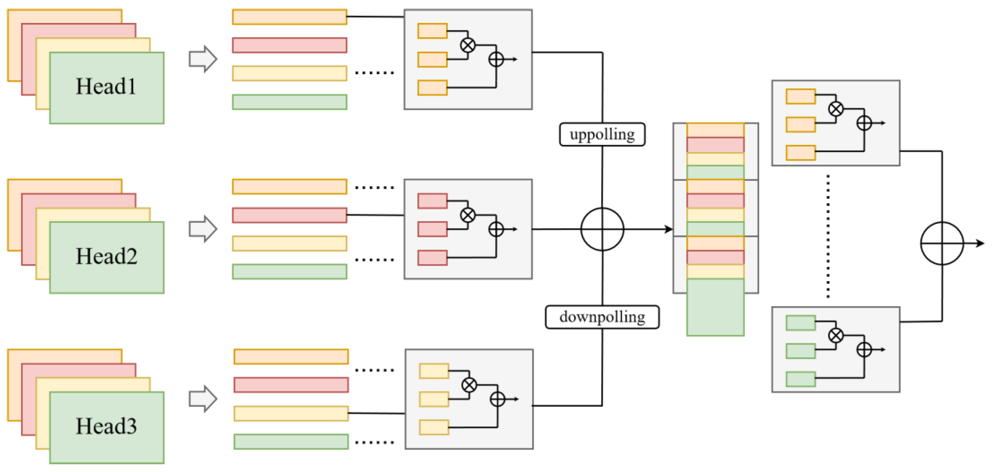
For each proposal, we extract a fixed-size ROI feature using ROI Align on the appropriate FPN level. These ROI features are then processed by the detection head, which has two branches, classification and regression. The classification branch (usually two fully connected layers and a softmax or sigmoid output) predicts the object class (or background). The regression branch is modified in our approach to include the Vector Decomposition Module (Section 3.4). Instead of predicting the standard 4 regression offsets for bounding box , our regression head predicts a set of vector parameters that describe the bounding box. Specifically, it predicts (, ) for the center offset (relative to the proposal center) and (, , , ) which are components of two vectors and emanating from the box center. These vectors, when combined with the center, define an oriented bounding box. The vector decomposition module takes these predictions and constructs the final detected bounding box (as an oriented box, which can be converted to a standard axis-aligned box for evaluation if needed). During training, this head is supervised to match the ground-truth boxes' vector representations.
In summary, our framework extends a standard two-level detector with the following new components. A GDConv layer for embedding the backbone for better feature extraction. An LBP module for texture enhancement and a vector-based bounding box regression header for orientation. The design is modular, and each component can be ablated or modified independently, as we will analyze in experiments.
3.2. Grouped Deformable Convolution (GDConv)
The grouped deformable convolution is a central component of our model, aiming to improve the backbone's ability to handle objects of varying shape and scale without incurring excessive computation. We build on the original deformable convolution operation [18]. A standard deformable convolution adds learnable offsets to the sampling locations of a convolution kernel. Formally, for a given convolution layer with kernel (of spatial size ) applied to an input feature map , a normal convolution at location computes, as shown in Equation 1.
where are the weights and ranges over the relative positions in the kernel. In a deformable convolution, each sampling location is shifted by an offset that is learned via an offset prediction convolution. The operation becomes Equation 2.
where is a fractional offset vector specific to position . These offsets are output by an auxiliary convolutional layer that takes the same input and produces channels (for the and offsets of each kernel point). This mechanism allows the convolution to sample features from a flexible receptive field shape, e.g., aligning along an object's contour or focusing on a small region if the object is small.
Figure 3.
The structure of the GDConv.
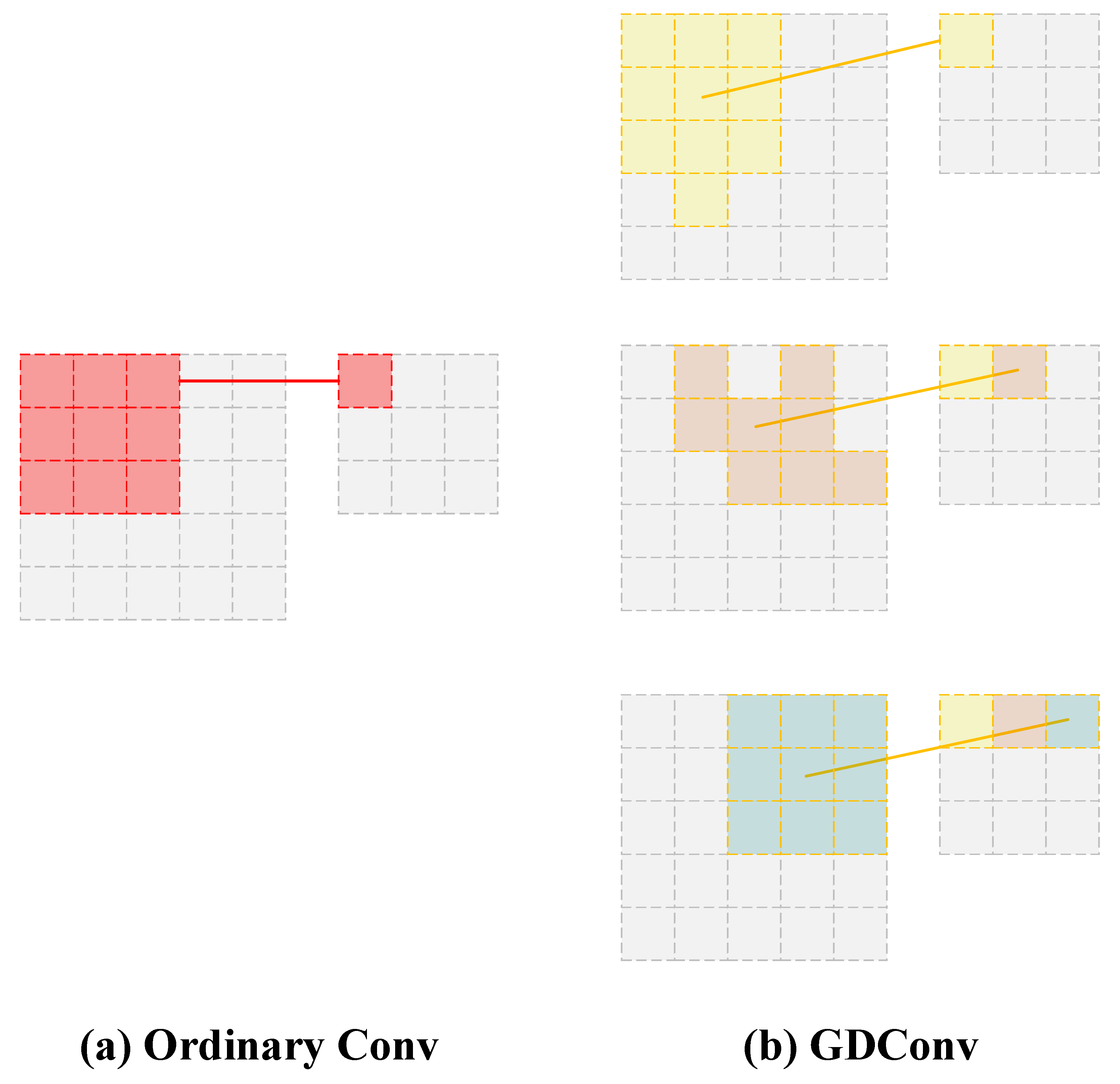
Our proposed GDConv modifies this by introducing the concept of groups in the deformable convolution filter. Instead of one monolithic deformable convolution over all input channels, we partition the input channels into groups (and similarly the output channels into groups for simplicity, such that each group of input channels maps to a group of output channels). For each group (where ), a separate deformable convolution is applied, as follow Equation 3.
where and denote the input and output feature maps restricted to group channels, and are the weights for group . Importantly, the offset can also be group-specific. In implementation, this means we have separate offset fields (each output by its own small convolution or a unified convolution that outputs values and we split them per group).
The benefit of grouping is two folds. On the one hand, for the parameter reduction. In a standard conv layer with input and output channels, the number of weights is. With G groups, each output channel only connects to inputs. Assuming is divisible by , the weight count becomes , which is of the original. Thus, grouping can dramatically reduce the parameters and computation if is large. We typically choose a moderate (e.g., 4 or 8) to balance efficiency and representation power.
On the other hand, different groups can learn to handle different types of features. In the context of SAR images, one group of filters and offsets might specialize in capturing large-scale structures (buildings, roads) by learning appropriate offsets (e.g., wider spread), while another group might focus on small objects (cars, signals) by learning offsets that hone in on fine details. Group-specific deformable offsets mean each group can deform its sampling grid in a different manner tailored to the subset of features it processes.
We apply GDConv in intermediate layers of the backbone where feature resolution and channel depth make it most beneficial. For example, the conv3 and conv4 stage, which produces medium-sized feature maps, is a good candidate in the ResNet backbone. These layers can see objects of different sizes and shapes, and increased deformability would help, while grouping reduces the added cost. By the conv5 stage, the feature map is very coarse (small spatially) and channels are high; one might still use GDConv there, though we found most benefits come from earlier stages.
GDConv is implemented by modifying the convolution layers in the network definition. During training, the offset convolution for each group learns to produce offsets that minimize the detection loss (indirectly, through backpropagation from the detection objective). We initialize the offsets to zero (so initially it behaves like a normal conv), and let the network gradually learn deformations. In our experiments, GDConv demonstrated the ability to deform to aligned with object orientations and scale regions. We observed offset vectors that elongate along vehicles and adjust around building boundaries, which validates the expected behavior.
3.3. LBP Enhancement Module
To better detect small objects and distinguish objects from background clutter, we incorporate Local Binary Pattern (LBP) features into the CNN. LBP is a classical operator that captures local texture by comparing each pixel with its neighbors [38]. In its basic form (with 8-connected neighborhood), the LBP value at pixel is computed by thresholding the patch around it.
where is the intensity of the center pixel, are the intensities of the 8 neighboring pixels, and is an indicator function that outputs 1 if the condition is true (neighbor pixel brighter or equal to center) or 0 otherwise. The result is an 8-bit code (0-255) describing the local pattern. This code can also be interpreted as a set of 8 binary features.
Our LBP module operates on a feature map to extract texture information that the CNN's learned filters might not explicitly capture. We choose a relatively high-resolution feature map from the backbone or FPN for this purpose. This map has a rich amount of detail about edges and small structures. We first transform this feature map to a single-channel representation suitable for LBP. One simple way is to take the intensity or the average across channels. In practice, we found that applying LBP on each channel separately and then aggregating was unnecessary; instead, we apply a convolution to collapse the feature map into one channel and then compute LBP on that.
Figure 4.
Overview of the LBP.
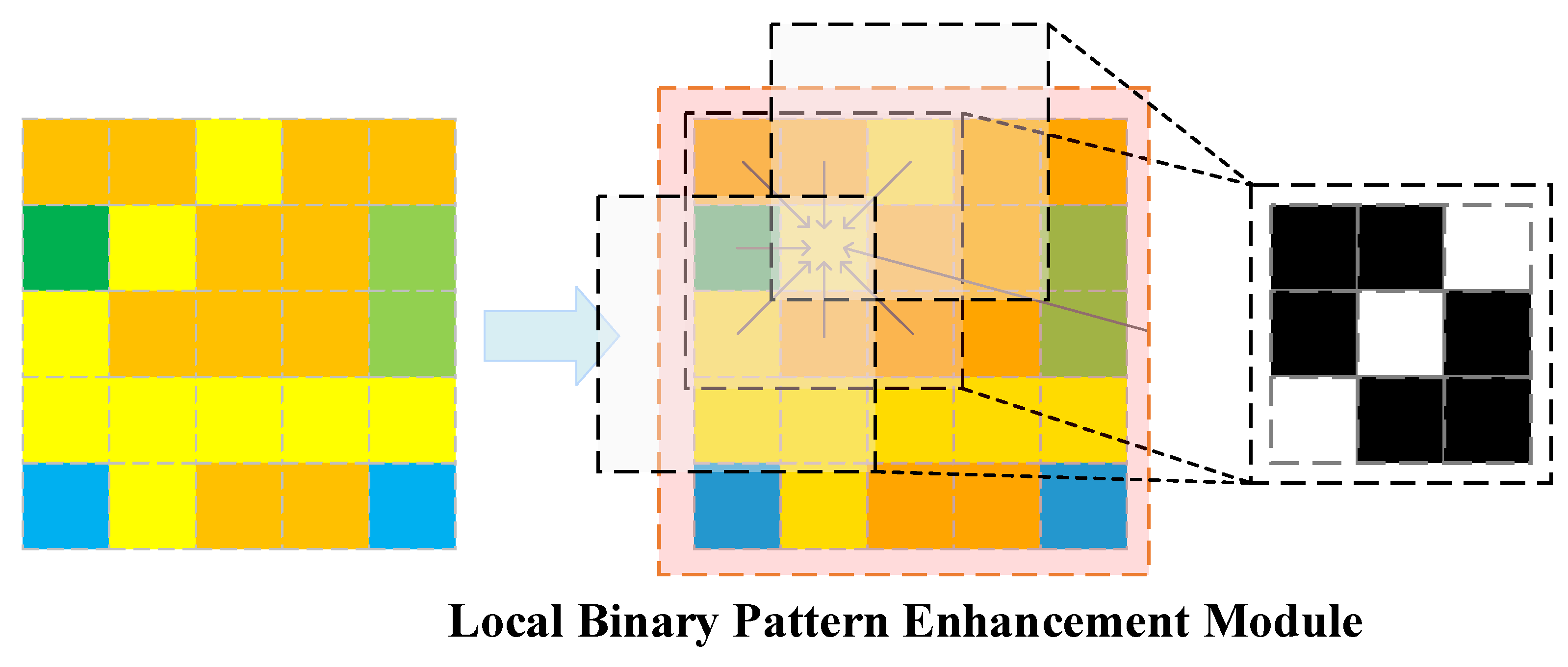
The LBP computation is implemented as a fixed (non-learnable) operation within the network. For each spatial location of the chosen feature map, we evaluate the 8 comparisons with its immediate neighbors. This yields 8 binary maps (one for each bit of the LBP code). We treat these 8 binary maps as 8 additional feature channels. These binary feature maps highlight local texture transitions; for example, one channel might indicate where a pixel is darker than its right neighbor, another where it is darker than its top neighbor, etc. Patterns like edges will produce distinctive streaks in these channels.
Next, we fuse the LBP features with the original CNN features. We concatenate the 8 LBP channels with the original feature map’s channels. This creates an augmented feature map with 256+8 channels. To avoid a disproportionate increase in dimensionality and to allow the network to learn how to best use these new features, we apply a convolution after concatenation. This convolution compresses the feature back to the original number of channels (256) or another desired dimension, and it learns the optimal weighting between original features and LBP features. In essence, this provides the network a chance to attend to LBP cues as needed. During training, the gradients flow through this fusion layer into both the previous CNN layers and the fixed LBP computation.
The effect of the LBP enhancement is that certain fine details become more salient. For example, in a SAR image, a small vehicle might produce a particular LBP pattern that helps it stand out from a similarly colored road. The CNN alone might not pick this up if the vehicle is only a few pixels, but the LBP will generate a strong binary pattern indicating an object boundary. By integrating this, our detector sees an improved feature representation. This typically leads to higher precision and higher recall for tiny objects. We will show in experiments that adding the LBP module yields a noticeable improvement especially on datasets with small objects.
It is worth noting that the LBP module adds negligible computational load. It involves simple comparisons and bitwise operations. There are no learned parameters in generating the LBP maps, and only a small overhead in memory for the additional channels. Therefore, it is an attractive plug-in module for improving feature richness without the risk of overfitting.
3.4. Vector Decomposition Module for Bounding Boxes
The vector decomposition module is our approach to predicting object bounding boxes, particularly to handle oriented objects. Traditional detectors parameterize a bounding box by , which are the relative offsets of the box center and the log-scale offsets of width and height with respect to some reference [2]. Some oriented detectors add a fifth parameter for the angle . However, predicting directly can be problematic due to the discontinuity at and because a small change in angle can cause a large change in box coordinates when the box is almost square. Instead, we opt for a vector-based representation that is smooth and continuous.
In our module, an object’s bounding box is represented by two vectors and originating from the box center (see Figure 1). These can be thought of as the directions towards two adjacent sides of the rotated rectangle. More concretely, let be the coordinates of the box center. We define as the vector from the center to the midpoint of the box’s first side, and as the vector from the center to the midpoint of the second side (which is the adjacent side, 90 degrees rotated from the first). In an oriented rectangle, these two vectors should be perpendicular and their lengths correspond to half of the box’s width and height, respectively. The four corners of the bounding box can be recovered as Equation 5.
where corresponds to width and to height. However, we do not enforce orthogonality or any explicit constraints in the prediction, this is learned implicitly. If the object is axis-aligned, might align with the horizontal such as and with the vertical . If the object is rotated by some angle, will rotate accordingly and should rotate by the same angle. In cases where the object does not have a clear orientation (or orientation is not annotated), the network is free to output any consistent pair that covers the object.
During training, we generate target vectors for each ground-truth box. For a horizontal ground-truth box, we set and in the coordinate frame of the proposal (i.e., relative to the proposal center and axes). Here , are the ground truth box width and height. For an oriented ground truth (if available, e.g., in a SAR dataset with oriented annotation), we compute and as half-length vectors along the ground truth box's orientation. These serve as regression targets for the network’s predictions.
Our detection head’s regression branch is thus modified to output 6 values per object . For class-specific regression, or 6 per class for class-specific, but we use class-agnostic regression for simplicity. are the center offset of the predicted box relative to the proposal’s center (just like in Faster R-CNN), encoded as , for ground truth (with denoting proposal, ground truth). For the vectors, we similarly normalize by the proposal size, as follow Equation 6.
as target values. The network outputs corresponding predictions which are then scaled back by to yield the predicted in absolute terms. (We treat each component as an independent regression task.)
One advantage of this approach is that it sidesteps the difficulty of angle prediction. If an object rotates gradually, the predicted vectors can rotate gradually as well, without any abrupt changes or wrapping around. Another advantage is that by predicting the full vectors, the model can, in principle, handle non-rectangular shapes or slight deviations if needed by adjusting .
At inference time, once we have for a proposal, we reconstruct the detection box. The predicted center is . The predicted vectors in absolute coordinates are , and similarly . We can directly output the oriented bounding box defined by and . For evaluation on datasets like VOC/COCO that expect axis-aligned boxes, we compute the axis-aligned bounding box that minimally encloses the oriented box.
The vector decomposition module adds a bit more output to the network, but this overhead is minor. We found that the network learns to predict perpendicular vectors for most objects, effectively learning the concept of oriented boxes. In cases where orientation is ambiguous, the network might output arbitrary perpendicular vectors which still yield a valid bounding box. This representation proved robust in our experiments, especially improving the localization of rotated objects. Additionally, even on datasets with only horizontal annotations, the vector approach did not harm performance; in fact, it slightly improved localization accuracy, likely because the model could adjust corners in a more flexible way than the standard width/height parameterization.
3.5. Loss Function
We train the entire network end-to-end using a multi-task loss that combines classification and localization terms, following the standard practice in two-stage detectors [2]. The overall loss is a sum of four components, as shown in Equation 7.
where RPN and ROI (region-of-interest) denote the proposal network and the second-stage detection head, respectively. We describe the latter two (ROI) in detail as they pertain to our contributions (the RPN uses standard losses as in Faster R-CNN).
For the classification branch of the ROI head, we use a cross-entropy loss over classes (plus background). For each predicted region , where is the softmax probability for the ground truth class (or the background class if the proposal does not match any object with ). We sum this over all ROI examples.
For the regression branch, we define a smooth L1 loss [51] on the vector parameters. Let be the predicted transformations for a given ROI, and the ground-truth transformation (as defined in Section 3.4). We use Equation 8.
We apply this regression loss only to positive ROIs (those matched to a ground-truth object). The SmoothL1 (Huber) loss [51] is defined as Equation 9.
which is less sensitive to outliers than L2 and is standard for box regression tasks.
The RPN is trained with a similar loss. Binary cross-entropy for object classification and SmoothL1 for regressing proposal coordinates. We weight the losses such that classification and regression contributions are roughly balanced. In practice, we set as the weight for the ROI regression loss relative to ROI classification, after normalizing by number of examples, which worked well (this follows the practice from Fast R-CNN [51]). The RPN loss is also weighted with .
No additional loss terms are needed for the LBP module or GDConv—those are implicitly learned through the effect they have on the detection accuracy. One could consider an auxiliary loss to encourage (perpendicular) or similar, but we found it unnecessary as the network naturally learns near-perpendicular vectors for rectangular objects to minimize regression error.
4. Experiments
We first validate the performance of the model on two major SAR small target detection datasets, HRSID and SSDD. Among them, an example of the dataset for SAR target detection is shown in Figure 5. Then, the generalization performance of the proposed model is validated on the remote sensing target detection dataset HRSC2016 and the natural image dataset Pascal VOC 2012.
4.1. Datasets and Implementation
We compare our model with baseline detectors and perform analyses to highlight the impact of each component. We use standard evaluation metrics including mean Average Precision (mAP) as well as Precision and Recall at a specified IoU threshold. In all experiments, our model is initialized from an ImageNet-pretrained ResNet-50 backbone. Unless otherwise noted, we use groups in GDConv layers, and include the LBP module and vector decomposition in all results for our model. The baseline for comparison is a Faster R-CNN with FPN [2,6] using the same ResNet-50 backbone but without deformable conv, without LBP, and with the standard box regression. We refer to our full model as GDConv+LBP+Vec and the baseline as Baseline (Faster R-CNN).
Our model is implemented in PyTorch. GDConv layers are inserted in the ResNet-50 at layers , replacing the conv in those blocks with a deformable conv of the same size and 4 groups. The LBP module is applied on the P3 feature; we reduce it to 1 channel and compute LBP using 8-neighborhood. The 8 binary maps are concatenated and passed through a conv to get back 256 channels. For vector decomposition, our ROI head outputs 6 regression values per ROI instead of 4. We still use class-agnostic regression for simplicity.
All models are trained with stochastic gradient descent (SGD). For VOC and COCO we train for 12 epochs. We apply standard data augmentations, horizontal flips for VOC/COCO and random scale jitter. For ImageNet, we did horizontal flips and multi-scale training. In inference, we use a single-scale and NMS with threshold 0.5 on final detections.
The HRSID dataset contains 5604 800×800 high-resolution images of 16,951 vessels. Its sources are a combination of Sentinel-1B (C-band) and TerraSAR-X & TanDEM-X (X-band) satellites, with pixel resolutions of 0.5 m, 1 m, and 3 m, covering a wide range of imaging angles and sea states. Horizontal frames, instance segmentation masks, and “in-shore/off-shore” scene labels are also provided, and 400 pure background images are attached for robustness testing.
SSDD [30] is a SAR small target detection dataset. A total of 1160 images are included, containing 2456 vessels, with an average of about 2.1 vessels per image. The labeling form is based on a horizontal surrounded frame, and the official new version also extends the rotated frame with pixel-level segmentation, which is convenient for studying small targets, dense targets, and fine localization. It is mainly derived from radar satellites RadarSat-2, TerraSAR-X, and Sentinel-1; the polarization modes cover HH/HV/VH/VV with a spatial resolution of 1 m-15 m, and the scenarios cover a wide range of sea states in the near-shore and far-shore.
The HRSC2016 dataset is a challenging remote sensing benchmark focused on ship detection in aerial images. It contains high-resolution images with significant variations in scale, orientation, and aspect ratio. One notable feature of HRSC2016 is that objects are labeled with oriented bounding boxes, making it an ideal testbed for evaluating the effectiveness of orientation-aware detection methods.
The VOC 2012 dataset [20] contains 20 object classes. We train on the VOC 2007+2012 trainval sets and evaluate on the VOC 2012 test set. As VOC annotations are axis-aligned, our model is trained with targets aligned to the horizontal/vertical box sides. We report results using the VOC metric of mAP at IoU = 0.5 (denoted ). Precision and recall are reported at IoU 0.5 as well, computed on the detection results.
4.2. Comparative Experiment
From the results shown in Table 1 and Table 2, our proposed model consistently outperforms a broad set of 17 state-of-the-art detection methods across all benchmark datasets. The superior performance has been achieved on SAR small target detection datasets HRSID and SSDD. In addition, including both remote sensing HRSC2016 dataset and natural image benchmarks dataset VOC2012. The improvements are evident across , precision, and recall. These gains can be attributed to the synergy between three architectural innovations in our design. These include Grouped Deformable Convolution (GDConv), Local Binary Pattern (LBP) enhancement module, and Vector Decomposition-based bounding box regression header, respectively.
In the high clutter, low signal-to-noise, and very small scale scenario of SAR small target test methods, our method is characterized by maintaining high-precision calls on both mainstream datasets. As shown in Table 1, the mAP50 of our method on the HRSID dataset is 90.9%. The mAP50 on the SSDD dataset is 87.2%, which exceeds the other 17 mainstream models of SOTA. Although both the HRSID and SSDD datasets are SAR small target detection datasets, the two sets of scenarios differ greatly, with the HRSID harbor/nearshore complexity and the SSDD offshore background monotony. The performance of our method is more stable, with cross-domain fluctuations of less than 4%. In addition, our method achieves 86.2% precision and 91.7% recall on HRSID. The precision on SSDD reaches 90.4%, and the recall reaches 90.7%. SAR applications are more afraid of misreporting ship shadows, and high precision directly reduces the burden of back-end screening. At the same time, the recall rate can be improved to avoid missed detection, which is also critical in maritime surveillance, compared with the traditional two-stage (Faster R-CNN 83%) of about 8%.
Our method maintains low drift for scene switching on both mainstream datasets, HRSID and SSDD. Compared with other mainstream models, it demonstrates the robustness to resolution differences, shoreline clutter, and imaging strong scattering on the SAR small target detection task. For traditional two-stage methods such as Faster R-CNN, we replace the traditional Neck with CMA rotated multiscale attention and SSJC semantic residual alignment to specifically enhance the small object response. This results in approximately 20% improvement in precision and approximately 10% improvement in recall. Compared to the YOLOv family of methods, DVDNet is able to achieve mAPs nearly equal to v6-n at only small/medium levels of parameter counts, approximately equal to YOLOv5s, while saving about 40% of FLOPs. This is well suited for shipboard/starboard real-time inference. In contrast to Transformer/DETR-like methods, we keep the CNN backbone as well as lightweight rotation attention, suppress background with a local prior, converge at high speed, and do not rely on tens of thousands of preheating steps.
It can be seen that the optimization is achieved between the combined precision and recall scores, cross-domain stability, and arithmetic consumption, even though the mAP alone is not maximized. When faced with tasks such as real-time maritime surveillance, vessel capturing, and satellite-carried SAR cruises, our approach provides a lower risk of underreporting and the overall advantage of being deployable on edge hardware.
On the HRSC2016 dataset, which presents unique challenges in remote sensing due to high-resolution imagery and densely packed, arbitrarily oriented ship targets, our model achieves the highest of 80.7%, surpassing all other methods, including the strong two-stage baselines such as Cascade R-CNN (80.6%), Sparse R-CNN (79.7%), and YOLOX-s (79.5%). Our model also achieves the best precision (85.0%) and recall (83.0%}), indicating both accurate localization and strong object coverage. These results confirm the effectiveness of our architecture in capturing fine-grained textures, geometric variances, and rotation patterns—key traits of SAR target detection.
On Pascal VOC 2012, a dataset characterized by axis-aligned annotations and limited object categories, our method still shows strong generalization, achieving a of 75.4%, outperforming all competing models by a significant margin. For instance, the next best result comes from Cascade R-CNN (68.7%) and Sparse R-CNN (68.6%), with our model improving the best baseline by 6.7%. This demonstrates that the proposed method is not overfitted to rotation-specific datasets, but rather yields universal improvements through its flexible feature and box modeling.
Figure 6 and Figure 7 show the visualization results on the two main SAR small target detection datasets. In the offshore dark scene of HRSID, the ships are only tiny specks. The model still gives more than 0.9 confidence, indicating that the GDConv adaptive sense field + LBP enhancement effectively improves the signal-to-noise ratio. The frame is aligned with the long axis of the hull in both the top-down “top-to-end” and oblique “bow-to-right” views, indicating that the vector decomposition regression head learns the rotation angle sufficiently to reduce the tilt IoU loss. This indicates that the vector decomposition regression head learns the rotation angle well enough to reduce the tilt IoU loss. In the visualization of the SSDD port, more than 10 ships are close to each other, bow to stern. The visualization shows that each ship is identified independently, and the spacing of the borders minimizes overlap. This validates the improved dense NMS strategy and small target feature fusion capability. In the strong scattering background or shoreline complex area, no mis-framing of buoys, shore walls, and wave tips is seen. The confidence distributions of both HRSID and SSDD domains are uniform, reflecting the robustness across resolution and pitch angle. This is enough to prove the core competitiveness of our model in SAR small target detection.
The HRSC2016 dataset and the VOC2012 dataset closely reflect the real-world challenges in remote sensing target detection and natural scene target detection. The main ones include extreme target aspect ratios and intensive position and orientation variations. The excellent results achieved by our method on HRSC2016 and VOC2012 validate the architectural decisions made, especially the combination of GDConv, LBP enhancement, and vector decomposition. The visualization results are shown in Figure 8 and Figure 9. It can be seen that the visualization results in both high-density, multi-directional ships in ports and daily multi-category scenarios are obtained with tight contours and low misdiagnosis, which directly corroborates the complementary advantages of these three modules for different domain characteristics. Secondly, there are minimal differences in confidence and border quality in the visualization results on different datasets. This confirms the ability of the model to migrate between SAR, remote sensing, and natural images. The 20-30 px miniature boat in Figure 8 and the distant basketball frame with bicycle in Figure 9 are all detected in their entirety. This contrasts with conventional detectors that tend to miss or drift frames at similar sizes, highlighting the significant improvement of this paper's test methods in the detection of small 10-30 px targets.
Cross-domain Generalization. The consistent performance on HRSID, SSDD, HRSC2016, and VOC2012 demonstrates that our model not only excels in the remote sensing domain but also exhibits strong generalization ability across natural scenes and varied detection challenges. This shows that the model can accurately catch extremely small vessels (10 – 30 px) in near-shore, high-clutter scenes. It can also rapidly lock onto sparse targets across wide-area offshore imagery. While many detectors perform well in specific domains, our method achieves top performance universally, making it a robust and transferable detection solution. This cross-domain capability is critical for real-world deployment, where model reliability across diverse environments is essential.
4.3. Ablation Experiment
To better understand the contribution of each proposed component, we conduct comprehensive ablation experiments on all four benchmark datasets. As shown in Table 3 and Table 4, we start from a plain Faster R-CNN baseline (“Nothing”) and incrementally add FPN, LBP, and GDConv modules. Each row in the table represents a specific configuration of active modules, allowing us to isolate the effects of individual and combined components.
Starting from the baseline, the model without any enhancement achieves relatively low performance. The of 62.2% on HRSID and 59.6% on VOC2012. When we introduce FPN alone, we observe clear improvements across all datasets. For example, on HRSC2016 the mAP rises from 55.2% to 66.6%, confirming that multi-scale feature fusion is essential for capturing object variability in size.
Incorporating the LBP module alone also brings measurable gains. For instance, the mAP on VOC2012 increases from 45.2% to 53.1%, and precision rises to 57.0%. This supports our hypothesis that local binary patterns enhance low-level contour information, improving object boundary discrimination.
The use of GDConv in isolation produces the most significant gain among single modules. On SSDD, GDConv boosts to 77.3%, with precision and recall also improving substantially. This demonstrates the effectiveness of spatially adaptive sampling and group-wise specialization for handling geometric variations in SAR targets.
The combination of LBP and GDConv leads to even more remarkable improvements. For example, on HRSID, increases to 89.5%, which is a 26.9% absolute improvement over the baseline. Similarly, on SSDD the combined model achieves 85.9% mAP, outperforming all partial variants.
Finally, the full model (FPN + LBP + GDConv), denoted as Ours, achieves the best performance across all benchmarks. The 90.9% mAP on HRSID, 87.2% on SSDD, 80.7% on HRSC2016, and 75.4% on VOC2012. Notably, the precision on HRSID reaches 90.9%, demonstrating that our method not only detects more targets but does so with fewer false positives.
The ablation study clearly demonstrates the incremental and complementary value of each proposed module. GDConv contributes most to spatial adaptability, LBP enhances texture sensitivity, and FPN provides strong multi-scale representations. Together, they form a synergistic and robust architecture that works well to achieve superior performance on all three types of datasets, SAR, remote sensing, and natural imagery.
5. Conclusions
In this paper, we propose DVDNet, a CNN-based unified framework for SAR target detection, which addresses small targets and arbitrary aspects in SAR images. The framework combines grouped deformable convolution, LBP texture enhancement module and vector decomposition based bounding box representation. DVDNet significantly improves the detection performance of standard architectures by combining the handling of multi-scale variations, arbitrary object orientations, and background complexity. DVDNet significantly improves detection performance through three major improvements. Introduction of grouped deformable convolution (GDConv), which allows the network to adaptively sample features while controlling parameters and computational overhead. Local Binary Pattern (LBP) is seamlessly embedded into the CNN to enhance the texture representation, improve the detection rate of small and dense targets, and reduce the texture background false detection. Adopting bounding box vector decomposition to represent the rotating box with two vectors pointing from the center to the edge, avoiding angular periodicity and locating targets in any direction more accurately. Extensive experiments with two mainstream SAR small target detection datasets, HRSID and SSDD, have demonstrated that each of the DVDNet components contributes to improved accuracy, providing state-of-the-art results for the ResNet-50 level detector. Notably, DVDNet, by combining fine-grained texture coding and adaptive sensing fields, shows particular strengths in detecting small objects, an area where many existing detectors perform poorly, as evidenced by the excellent results on the HRSID dataset and the SSDD dataset. The generalization performance is also validated on the remote sensing dataset HRSC2016 and the natural scene dataset VOC2012.
References
- R. Girshick, J. R. Girshick, J. Donahue, T. Darrell, and J. Malik, "Rich feature hierarchies for accurate object detection and semantic segmentation," in Proceedings of the IEEE conference on computer vision and pattern recognition, pp. 580-587, 2014. [CrossRef]
- S. Ren, K. S. Ren, K. He, R. Girshick, and J. Sun, "Faster r-cnn: Towards real-time object detection with region proposal networks," Advances in neural information processing systems, vol. 28, 2015. [CrossRef]
- J. Redmon, S. J. Redmon, S. Divvala, R. Girshick, and A. Farhadi, "You only look once: Unified, real-time object detection," in Proceedings of the IEEE conference on computer vision and pattern recognition, pp. 779-788, 2016. [CrossRef]
- B. Wu, J. B. Wu, J. Huang, and Q. Duan, "Real-time Intelligent Healthcare Enabled by Federated Digital Twins with AoI Optimization," IEEE Network, pp. 1-1, 2025. [CrossRef]
- B. Wu, Z. B. Wu, Z. Cai, W. Wu, and X. Yin, "AoI-aware resource management for smart health via deep reinforcement learning," IEEE Access, 2023. [CrossRef]
- T.-Y. Lin, P. T.-Y. Lin, P. Dollar, R. Girshick, K. He, B. Hariharan, and S. Belongie, "Feature pyramid networks for object detection," in Proceedings of the IEEE conference on computer vision and pattern recognition, pp. 2117-2125, 2017.
- J. Ding, N. J. Ding, N. Xue, Y. Long, G.-S. Xia, and Q. Lu, "Learning roi transformer for oriented object detection in aerial images," in Proceedings of the IEEE/CVF conference on computer vision and pattern recognition, pp. 2849-2858, 2019. [CrossRef]
- J. Huang, B. J. Huang, B. Wu, Q. Duan, L. Dong, and S. Yu, "A Fast UAV Trajectory Planning Framework in RIS-assisted Communication Systems with Accelerated Learning via Multithreading and Federating," IEEE Transactions on Mobile Computing, pp. 1-16, 2025. [CrossRef]
- X. Yang, J. X. Yang, J. Yang, J. Yan, Y. Zhang, T. Zhang, Z. Guo, X. Sun, and K. Fu, "Scrdet: Towards more robust detection for small, cluttered and rotated objects," in Proceedings of the IEEE/CVF International Conference on Computer Vision, pp. 8232-8241, 2019. [CrossRef]
- D. Liang, M. D. Liang, M. Hashimoto, K. Iwata, X. Zhao, et al., "Co-occurrence probability-based pixel pairs background model for robust object detection in dynamic scenes," Pattern Recognition, vol. 48, no. 4, pp. 1374-1390, 2015. [CrossRef]
- B. Wu, J. B. Wu, J. Huang, and Q. Duan, "FedTD3: An Accelerated Learning Approach for UAV Trajectory Planning," in International Conference on Wireless Artificial Intelligent Computing Systems and Applications (WASA), pp. 13-24, Springer, 2025. [CrossRef]
- Z. Fang, S. Z. Fang, S. Hu, J. Wang, Y. Deng, X. Chen, and Y. Fang, "Prioritized Information Bottleneck Theoretic Framework With Distributed Online Learning for Edge Video Analytics," IEEE Transactions on Networking, pp. 1-17, 2025. [CrossRef]
- B. Wu and W. Wu, "Model-Free Cooperative Optimal Output Regulation for Linear Discrete-Time Multi-Agent Systems Using Reinforcement Learning," Mathematical Problems in Engineering, vol. 2023, no. 1, p. 6350647, 2023. [CrossRef]
- H. Li, J. H. Li, J. Chen, A. Zheng, Y. Wu, and Y. Luo, "Day-night cross-domain vehicle re-identification," in Proceedings of the IEEE/CVF Conference on Computer Vision and Pattern Recognition, pp. 12626-12635, 2024. [CrossRef]
- T.-Y. Lin, P. T.-Y. Lin, P. Dollar, R. Girshick, K. He, B. Hariharan, and S. Belongie, "Feature pyramid networks for object detection," in Proceedings of the IEEE Conference on Computer Vision and Pattern Recognition, pp. 2117-2125, 2017.
- D. Pan, B.-N. D. Pan, B.-N. Wu, Y.-L. Sun, and Y.-P. Xu, "A fault-tolerant and energy-efficient design of a network switch based on a quantum-based nano-communication technique," Sustainable Computing: Informatics and Systems, vol. 37, p. 100827, 2023. [CrossRef]
- B. Wu, J. B. Wu, J. Huang, Q. Duan, L. Dong, and Z. A: Cai, "Enhancing vehicular platooning with wireless federated learning; arXiv:2507.00856. [CrossRef]
- J. Dai, H. J. Dai, H. Qi, Y. Xiong, Y. Li, G. Zhang, H. Hu, and Y. Wei, "Deformable convolutional networks," in Proceedings of the IEEE International Conference on Computer Vision, pp. 764-773, 2017. [CrossRef]
- S. Xie, R. S. Xie, R. Girshick, P. Dollar, Z. Tu, and K. He, "Aggregated residual transformations for deep neural networks," in Proceedings of the IEEE Conference on Computer Vision and Pattern Recognition, pp. 1492-1500, 2017. [CrossRef]
- M. Everingham, L. M. Everingham, L. Van Gool, C. K. Williams, J. Winn, and A. Zisserman, "The pascal visual object classes (voc) challenge," International Journal of Computer Vision, vol. 88, pp. 303-338, 2010. [CrossRef]
- T.-Y. Lin, M. T.-Y. Lin, M. Maire, S. Belongie, J. Hays, P. Perona, D. Ramanan, P. Dollar, and C. L. Zitnick, "Microsoft coco: Common objects in context," in *Computer Vision–ECCV 2014: 13th European Conference, Zurich, Switzerland, -12, 2014, Proceedings, Part V 13*, pp. 740-755, Springer, 2014. 6 September. [CrossRef]
- Russakovsky, J.A. Deng, H. Su, J. Krause, S. Satheesh, S. Ma, Z. Huang, A. Karpathy, A. Khosla, M. Bernstein, et al., "Imagenet large scale visual recognition challenge," International Journal of Computer Vision, vol. 115, pp. 211-252, 2015. [CrossRef]
- Y. Liu, P. Y. Liu, P. Sun, N. Wergeles, and Y. Shang, "A survey and performance evaluation of deep learning methods for small object detection," Expert Systems with Applications, vol. 172, p. 114602, 2021. [CrossRef]
- G. Cheng, X. G. Cheng, X. Yuan, X. Yao, K. Yan, Q. Zeng, X. Xie, and J. Han, "Towards large-scale small object detection: Survey and benchmarks," IEEE Transactions on Pattern Analysis and Machine Intelligence, vol. 45, no. 11, pp. 13467-13488, 2023. [CrossRef]
- F. Ozge Unel, B. O. F. Ozge Unel, B. O. Ozkalayci, and C. Cigla, "The power of tiling for small object detection," in Proceedings of the IEEE/CVF Conference on Computer Vision and Pattern Recognition Workshops, pp. 0-0, 2019. [CrossRef]
- C. Chen, M.-Y. C. Chen, M.-Y. Liu, O. Tuzel, and J. Xiao, "R-cnn for small object detection," in Asian Conference on Computer Vision, pp. 214-230, Springer, 2016. [CrossRef]
- X. Yang, J. X. Yang, J. Yang, J. Yan, Y. Zhang, T. Zhang, Z. Guo, X. Sun, and K. Fu, "Scrdet: Towards more robust detection for small, cluttered and rotated objects," in Proceedings of the IEEE/CVF International Conference on Computer Vision, pp. 8232-8241, 2019. [CrossRef]
- R. Garg, S. M. R. Garg, S. M. Seitz, D. Ramanan, and N. Snavely, "Where's waldo: matching people in images of crowds," in CVPR 2011, pp. 1793-1800, IEEE, 2011. [CrossRef]
- P. Parnes, K. P. Parnes, K. Synnes, and D. Schefstrom, "mStar: Enabling collaborative applications on the Internet," IEEE Internet Computing, vol. 4, no. 5, pp. 32-39, 2000. [CrossRef]
- Y. Mao, X. Y. Mao, X. Li, H. Su, et al., "Ship detection for SAR imagery based on deep learning: A benchmark," in 2020 IEEE 9th Joint International Information Technology and Artificial Intelligence Conference (ITAIC), vol. 9, pp. 1934-1940, IEEE, 2020. [CrossRef]
- J. Leng, Y. J. Leng, Y. Ye, M. Mo, C. Gao, J. Gan, B. Xiao, and X. Gao, "Recent advances for aerial object detection: A survey," ACM Computing Surveys, vol. 56, no. 12, pp. 1-36, 2024. [CrossRef]
- X. Zhu, H. X. Zhu, H. Hu, S. Lin, and J. Dai, "Deformable convnets v2: More deformable, better results," in Proceedings of the IEEE/CVF Conference on Computer Vision and Pattern Recognition, pp. 9308-9316, 2019. [CrossRef]
- J. Dai, H. J. Dai, H. Qi, Y. Xiong, Y. Li, G. Zhang, H. Hu, and Y. Wei, "Deformable convolutional networks," in Proceedings of the IEEE International Conference on Computer Vision, pp. 764-773, 2017. [CrossRef]
- X. Wang, K. C. X. Wang, K. C. Chan, K. Yu, C. Dong, and C. Change Loy, "Edvr: Video restoration with enhanced deformable convolutional networks," in Proceedings of the IEEE/CVF Conference on Computer Vision and Pattern Recognition Workshops, pp. 0-0, 2019. [CrossRef]
- X. Zhu, H. X. Zhu, H. Hu, S. Lin, and J. Dai, "Deformable convnets v2: More deformable, better results," in Proceedings of the IEEE/CVF Conference on Computer Vision and Pattern Recognition, pp. 9308-9316, 2019. [CrossRef]
- N. Ma, X. N. Ma, X. Zhang, H.-T. Zheng, and J. Sun, "Shufflenet v2: Practical guidelines for efficient cnn architecture design," in Proceedings of the European Conference on Computer Vision (ECCV), pp. 116-131, 2018. [CrossRef]
- G. Zhang, S. G. Zhang, S. Lu, and W. Zhang, "Cad-net: A context-aware detection network for objects in remote sensing imagery," IEEE Transactions on Geoscience and Remote Sensing, vol. 57, no. 12, pp. 10015-10024, 2019. [CrossRef]
- T. Ojala, M. T. Ojala, M. Pietikainen, and T. Maenpaa, "Multiresolution gray-scale and rotation invariant texture classification with local binary patterns," IEEE Transactions on Pattern Analysis and Machine Intelligence, vol. 24, no. 7, pp. 971-987, 2002. [CrossRef]
- N. Dalal and B. Triggs, "Histograms of oriented gradients for human detection," in 2005 IEEE Computer Society Conference on Computer Vision and Pattern Recognition (CVPR'05), vol. 1, pp. 886-893, IEEE, 2005. [CrossRef]
- T. Ojala, M. T. Ojala, M. Pietikainen, and T. Maenpaa, "Multiresolution gray-scale and rotation invariant texture classification with local binary patterns," IEEE Transactions on Pattern Analysis and Machine Intelligence, vol. 24, no. 7, pp. 971-987, 2002. [CrossRef]
- T. Ojala, M. T. Ojala, M. Pietikainen, and T. Maenpaa, "Gray scale and rotation invariant texture classification with local binary patterns," in *Computer Vision-ECCV 2000: 6th European Conference on Computer Vision Dublin, Ireland, -July 1, 2000 Proceedings, Part I 6*, pp. 404-420, Springer, 2000. 26 June. [CrossRef]
- C. Szegedy, W. C. Szegedy, W. Liu, Y. Jia, P. Sermanet, S. Reed, D. Anguelov, D. Erhan, V. Vanhoucke, and A. Rabinovich, "Going deeper with convolutions," in Proceedings of the IEEE Conference on Computer Vision and Pattern Recognition, pp. 1-9, 2015. [CrossRef]
- Oztel, G.I. Yolcu Oztel, and D. Akgun, "A hybrid lbp-dcnn based feature extraction method in yolo: An application for masked face and social distance detection," Multimedia Tools and Applications, vol. 82, no. 1, pp. 1565-1583, 2023. [CrossRef]
- E. Nichani, A. E. Nichani, A. Radhakrishnan, and C. Uhler, "Do deeper convolutional networks perform better?," in International Conference on Machine Learning, 2021. [CrossRef]
- G. Zhao and M. Pietikainen, "Dynamic texture recognition using local binary patterns with an application to facial expressions," IEEE Transactions on Pattern Analysis and Machine Intelligence, vol. 29, no. 6, pp. 915-928, 2007. [CrossRef]
- K. Zhou, M. K. Zhou, M. Zhang, Y. Dong, J. Tan, S. Zhao, and H. Wang, "Vector decomposition-based arbitrary-oriented object detection for optical remote sensing images," Remote Sensing, vol. 15, no. 19, p. 4738, 2023. [CrossRef]
- N. Li, S. N. Li, S. Jiang, J. Xue, S. Ye, and S. Jia, "Texture-aware self-attention model for hyperspectral tree species classification," IEEE Transactions on Geoscience and Remote Sensing, vol. 62, pp. 1-15, 2023. [CrossRef]
- F. Zhou, Q. F. Zhou, Q. Chen, B. Liu, and G. Qiu, "Structure and texture-aware image decomposition via training a neural network," IEEE Transactions on Image Processing, vol. 29, pp. 3458-3473, 2019. [CrossRef]
- J. Yi, P. J. Yi, P. Wu, B. Liu, Q. Huang, H. Qu, and D. Metaxas, "Oriented object detection in aerial images with box boundary-aware vectors," in Proceedings of the IEEE/CVF Winter Conference on Applications of Computer Vision, pp. 2150-2159, 2021. [CrossRef]
- W. Li, Y. W. Li, Y. Chen, K. Hu, and J. Zhu, "Oriented reppoints for aerial object detection," in Proceedings of the IEEE/CVF Conference on Computer Vision and Pattern Recognition, pp. 1829-1838, 2022. [CrossRef]
- R. Girshick, "Fast r-cnn," in Proceedings of the IEEE International Conference on Computer Vision, pp. 1440-1448, 2015. [CrossRef]
Figure 1.
Overview of the proposed detection framework.
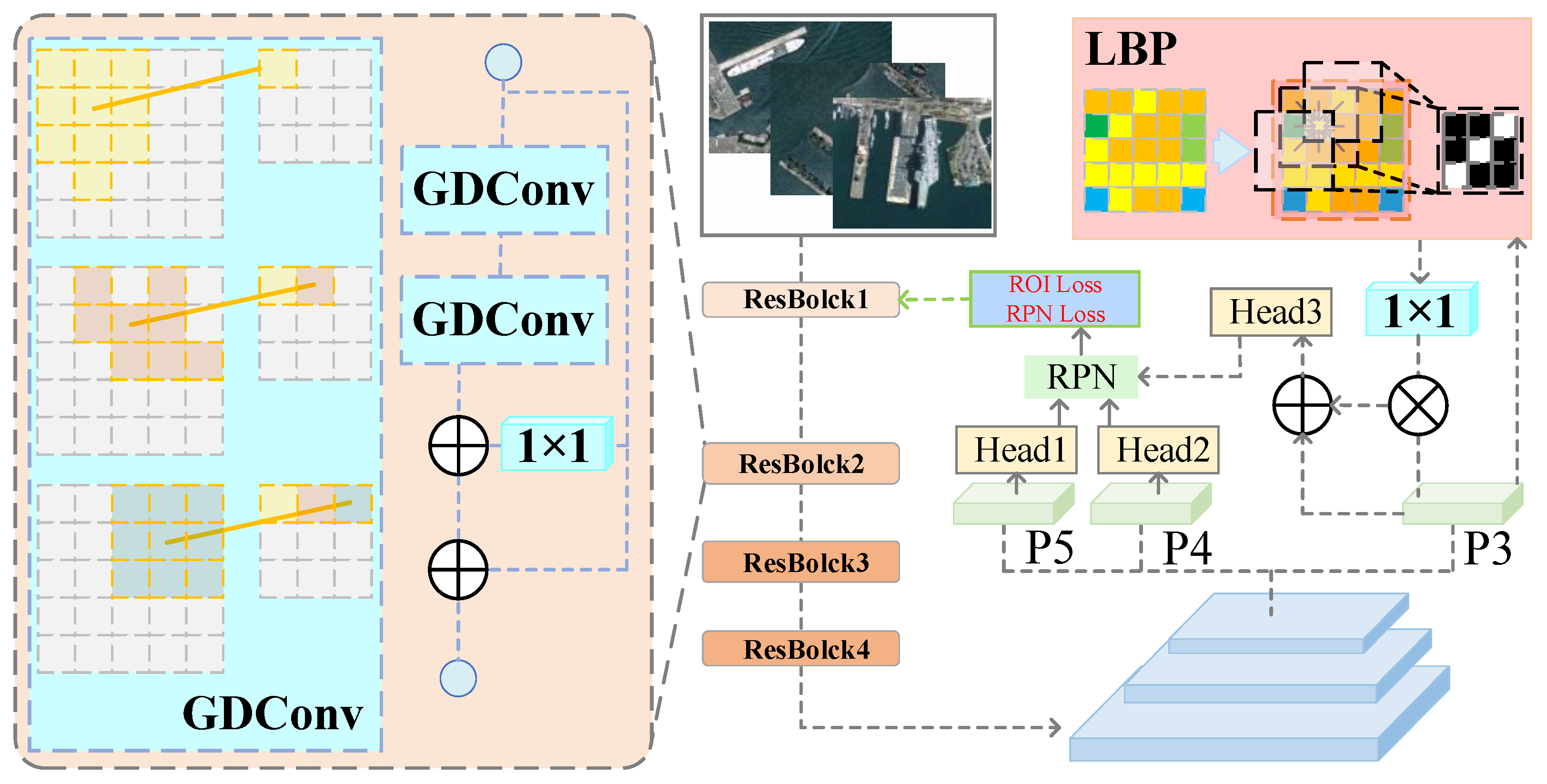
Figure 5.
Samples on the HRSID and SSDD datasets.
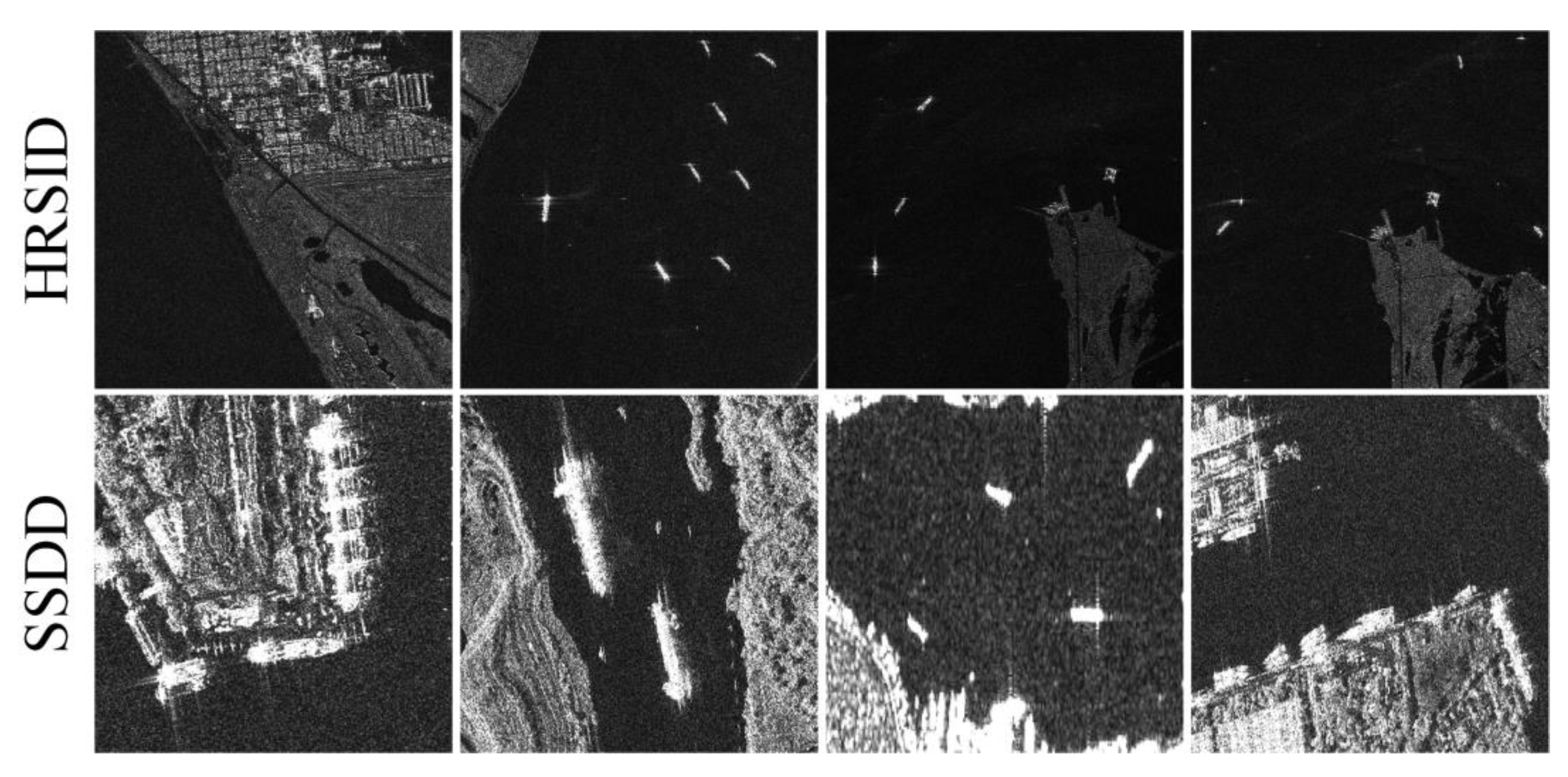
Figure 6.
Visualization of detection results of the DVDNet on HRSID dataset visualization.
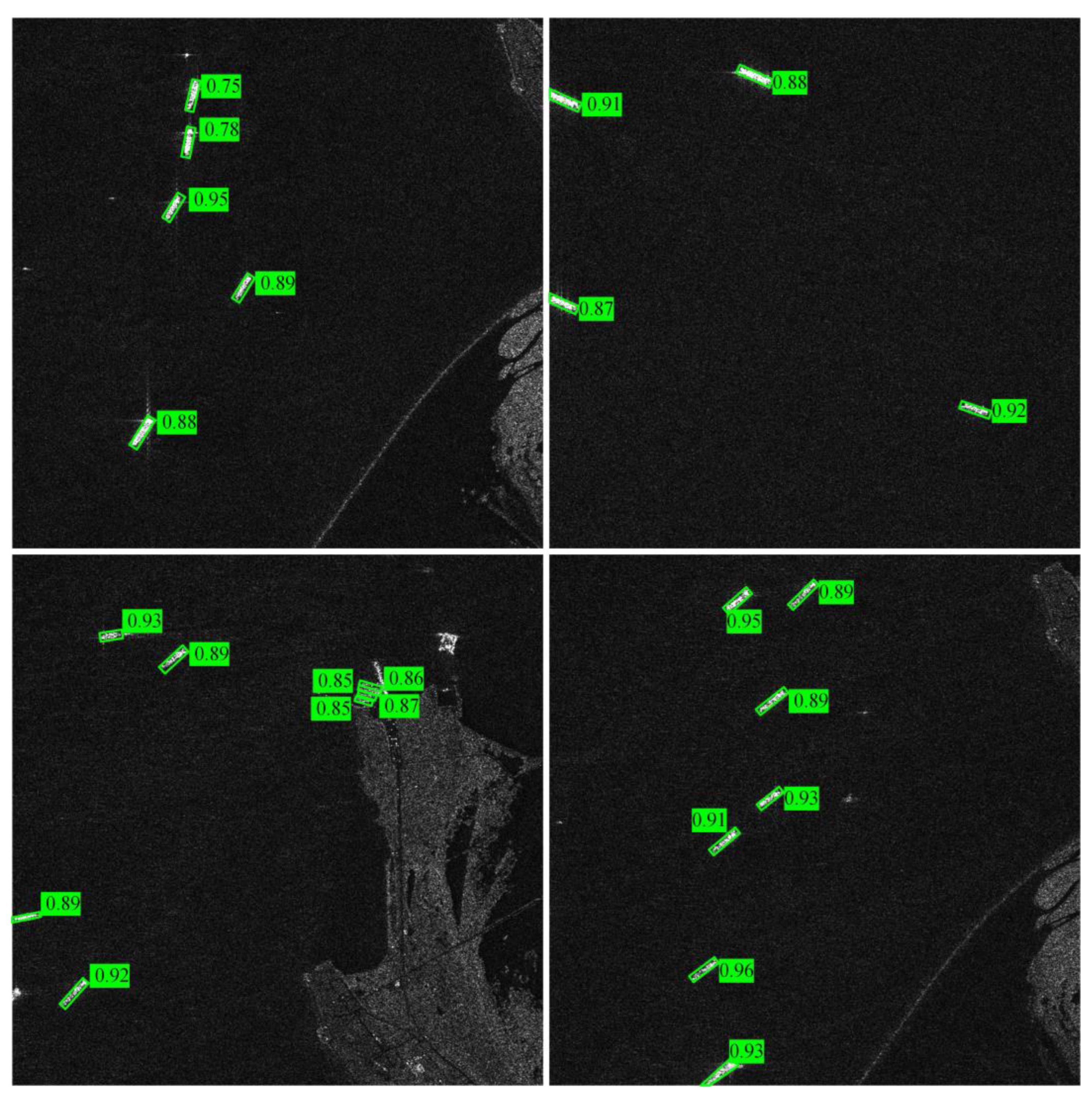
Figure 7.
Visualization of detection results of the DVDNet on SSDD dataset visualization.
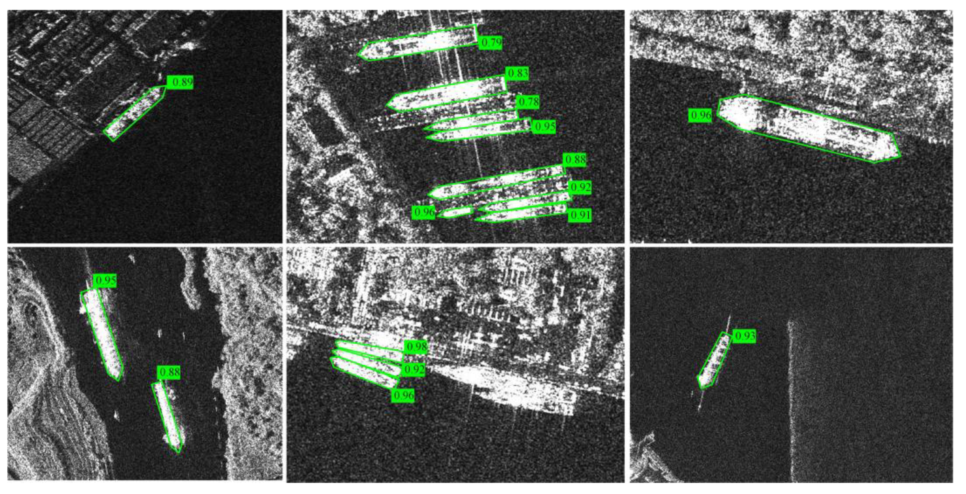
Figure 8.
Visualization of detection results of our model on the HRSC2016 dataset.
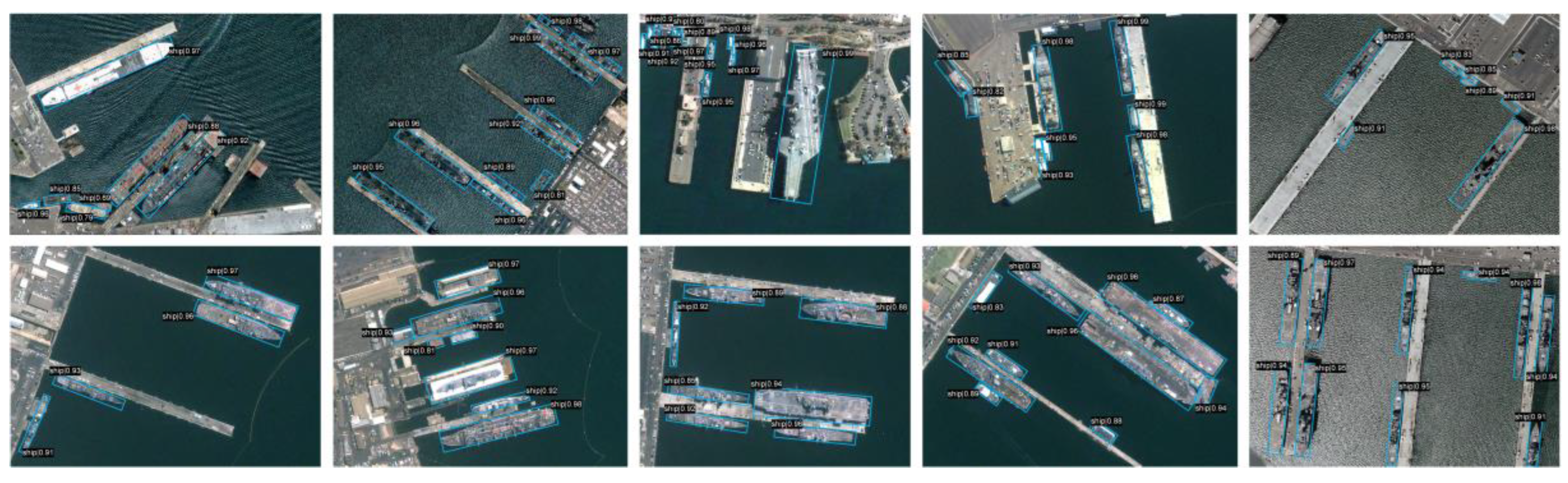
Figure 9.
Visualization of detection results of our model on VOC2012 dataset visualization.

Table 1.
Comparison of 18 detection methods on the HRSID and SSDD test sets. Results are reported as mAP, precision, and recall at IoU = 0.5.
Table 1.
Comparison of 18 detection methods on the HRSID and SSDD test sets. Results are reported as mAP, precision, and recall at IoU = 0.5.
| Method | HRSID | SSDD | ||||
|---|---|---|---|---|---|---|
| mAP50 | Precision | Recall | mAP50 | Precision | Recall | |
| YOLOv5s | 89.5% | 83.1% | 91.3% | 72.9% | 58.8% | 77.9% |
| YOLOv6-n | 89.9% | 85.5% | 91.4% | 82.0% | 87.2% | 86.4% |
| YOLOv7-tiny | 83.6% | 85.5% | 74.6% | 83.7% | 81.1% | 84.9% |
| YOLOv8n | 90.4% | 86.0% | 91.7% | 87.0% | 85.0% | 84.0% |
| YOLOX-s | 88.9% | 82.6% | 90.4% | 74.0% | 66.0% | 77.4% |
| CenterNet | 83.8% | 66.3% | 86.8% | 72.6% | 61.5% | 76.8% |
| FCOS | 82.1% | 76.2% | 85.1% | 69.5% | 53.1% | 76.0% |
| SSD300 | 80.0% | 70.5% | 84.5% | 67.2% | 52.3% | 75.4% |
| RetinaNet | 82.5% | 72.0% | 85.0% | 71.8% | 58.2% | 73.6% |
| Faster R-CNN | 80.5% | 66.9% | 83.4% | 69.5% | 67.2% | 74.2% |
| Cascade R-CNN | 86.0% | 74.0% | 87.8% | 76.4% | 70.0% | 78.8% |
| DETR | 81.0% | 70.0% | 80.0% | 71.0% | 60.2% | 78.3% |
| Deformable DETR | 89.1% | 84.3% | 90.0% | 79.8% | 84.2% | 81.9% |
| Sparse R-CNN | 85.0% | 78.0% | 86.0% | 78.0% | 73.0% | 79.0% |
| Dynamic R-CNN | 82.0% | 72.0% | 82.0% | 73.9% | 70.0% | 77.0% |
| GCNet | 81.5% | 70.0% | 82.0% | 75.0% | 65.2% | 79.0% |
| Libra R-CNN | 82.5% | 71.0% | 83.0% | 75.5% | 66.8% | 78.3% |
| DVDNet (Ours) | 90.9% | 86.2% | 91.7% | 87.2% | 90.4% | 90.7% |
Table 2.
Comparison of 18 detection methods on the HRSC2016 and Pascal VOC 2012 test sets. Results are reported as mAP, precision, and recall at IoU = 0.5.
Table 2.
Comparison of 18 detection methods on the HRSC2016 and Pascal VOC 2012 test sets. Results are reported as mAP, precision, and recall at IoU = 0.5.
| Method | HRSC2016 | VOC2012 | ||||
|---|---|---|---|---|---|---|
| mAP50 | Precision | Recall | mAP50 | Precision | Recall | |
| YOLOv5s | 78.4% | 83.1% | 80.6% | 66.9% | 61.0% | 68.8% |
| YOLOv6-n | 78.1% | 82.7% | 80.2% | 66.3% | 60.5% | 68.0% |
| YOLOv7-tiny | 78.9% | 83.4% | 80.9% | 67.1% | 61.3% | 69.1% |
| YOLOv8n | 79.0% | 83.3% | 80.4% | 67.3% | 61.7% | 69.5% |
| YOLOX-s | 79.5% | 84.1% | 81.2% | 68.0% | 62.3% | 60.0% |
| CenterNet | 77.2% | 81.2% | 78.8% | 66.2% | 70.2% | 68.1% |
| FCOS | 78.3% | 82.6% | 80.2% | 67.5% | 61.5% | 69.2% |
| SSD300 | 74.1% | 79.0% | 76.3% | 64.9% | 70.0% | 70.7% |
| RetinaNet | 77.8% | 82.3% | 79.6% | 66.7% | 60.9% | 67.2% |
| Faster R-CNN | 79.2% | 84.0% | 81.1% | 67.8% | 61.8% | 69.9% |
| Cascade R-CNN | 80.6% | 84.5% | 82.5% | 68.7% | 62.5% | 60.9% |
| DETR | 78.5% | 83.0% | 80.3% | 68.1% | 62.4% | 70.4% |
| Deformable DETR | 79.8% | 84.2% | 81.9% | 68.9% | 63.0% | 70.9% |
| Sparse R-CNN | 79.7% | 84.3% | 81.6% | 68.6% | 73.0% | 71.0% |
| Dynamic R-CNN | 79.3% | 83.7% | 81.0% | 68.2% | 72.6% | 70.3% |
| GCNet | 78.7% | 82.9% | 80.5% | 67.0% | 60.8% | 68.2% |
| Libra R-CNN | 78.8% | 83.0% | 80.8% | 67.2% | 61.1% | 68.9% |
| DVDNet (Ours) | 80.7% | 85.0% | 83.0% | 75.4% | 74.7% | 72.7% |
Table 3.
Ablation experiment on the HRSID and SSDD test sets. Results are reported as mAP, precision, and recall at IoU = 0.5.
Table 3.
Ablation experiment on the HRSID and SSDD test sets. Results are reported as mAP, precision, and recall at IoU = 0.5.
| Combination | FPN | LBP | GDConv | HRSID | SSDD | ||||
| mAP50 | Precision | Recall | mAP50 | Precision | Recall | ||||
| None | 62.2% | 61.4% | 64.5% | 59.6% | 64.3% | 63.8% | |||
| FPN | √ | 75.0% | 62.1% | 65.5% | 72.0% | 65.1% | 64.8% | ||
| LBP | √ | 64.3% | 62.9% | 65.7% | 61.7% | 65.9% | 65.0% | ||
| GDConv | √ | 76.6% | 73.8% | 78.1% | 73.5% | 77.4% | 77.3% | ||
| LBP+GDConv | √ | √ | 89.5% | 74.9% | 79.0% | 85.9% | 78.6% | 78.1% | |
| DVDNet | √ | √ | √ | 90.9% | 86.2% | 91.7% | 87.2% | 90.4% | 90.7% |
Table 4.
Ablation experiment on the HRSC2016 and VOC2012 test sets. Results are reported as mAP, precision, and recall at IoU = 0.5.
Table 4.
Ablation experiment on the HRSC2016 and VOC2012 test sets. Results are reported as mAP, precision, and recall at IoU = 0.5.
| Combination | FPN | LBP | GDConv | HRSC2016 | VOC2012 | ||||
| mAP50 | Precision | Recall | mAP50 | Precision | Recall | ||||
| None | 55.2% | 60.5% | 58.4% | 45.2% | 50.5% | 68.4% | |||
| FPN | √ | 66.6% | 61.2% | 59.3% | 56.6% | 51.2% | 59.3% | ||
| LBP | √ | 57.1% | 62.0% | 59.5% | 53.1% | 57.0% | 56.4% | ||
| GDConv | √ | 68.0% | 72.8% | 70.7% | 64.4% | 62.5% | 63.4% | ||
| LBP+GDConv | √ | √ | 79.5% | 73.9% | 71.5% | 67.4% | 73.9% | 71.5% | |
| DVDNet | √ | √ | √ | 80.7% | 85.0% | 83.0% | 75.4% | 74.7% | 72.7% |
Disclaimer/Publisher’s Note: The statements, opinions and data contained in all publications are solely those of the individual author(s) and contributor(s) and not of MDPI and/or the editor(s). MDPI and/or the editor(s) disclaim responsibility for any injury to people or property resulting from any ideas, methods, instructions or products referred to in the content. |
© 2025 by the authors. Licensee MDPI, Basel, Switzerland. This article is an open access article distributed under the terms and conditions of the Creative Commons Attribution (CC BY) license (http://creativecommons.org/licenses/by/4.0/).
Copyright: This open access article is published under a Creative Commons CC BY 4.0 license, which permit the free download, distribution, and reuse, provided that the author and preprint are cited in any reuse.


