
Submitted:
18 December 2024
Posted:
19 December 2024
You are already at the latest version
Abstract
Compared to natural images, aircraft targets in Synthetic Aperture Radar (SAR) images are typically smaller and surrounded by complex backgrounds. Directly applying object detection algorithms based on optical images to SAR images often results in poor detection accuracy and inaccurate target localization. One of the reasons for this issue is that current networks do not fully utilize the semantic information between the target and background in the feature space. To address this problem, this paper proposes the FCCS-YOLO algorithm based on YOLOv8. Firstly, FCCS-YOLO optimizes the target detection layers of YOLOv8 to make it more suitable for small and medium-sized aircraft targets in SAR images. Secondly, the Conv-Passthrough-DSC(CPD) module is proposed as the primary downsampling structure to address the reduced receptive field caused by adjustments in the feature detection layers and to overcome the limitations of current mainstream downsampling structures. Thirdly, the Skew Intersection over Union (SIOU) loss function is introduced to further enhance the bounding box regression capability. Finally, a contrastive learning regularization method is proposed for aircraft detection in SAR images. This method not only addresses the impact of feature consistency on bounding box regression but also improves the network’s ability to perceive feature differences across categories. Experimental results show that the FCCS-YOLO model performs excellently across multiple evaluation metrics.
Keywords:
SAR Images
; Deep Learning
; Aircraft Target Detection
; Contrastive Learning
1. Introduction
Synthetic Aperture Radar (SAR) is unaffected by weather and time, making it one of the key tools for modern reconnaissance. It plays an increasingly important role in remote sensing [1]. Through years of technological innovation, SAR systems have made significant advancements in resolution, polarization, and operational modes, enabling the acquisition of high-resolution SAR images [2]. Aircraft, as an important type of target, has considerable value in both civilian and military domains, and aircraft detection is helpful for the effective airport management in civilian field and the combat and deployment in military applications [3]. Therefore, precise detection of aircraft targets in high-resolution SAR images has substantial practical significance.
In the field of target detection in SAR images, there are two main types of approaches: traditional methods and deep learning methods. Traditional SAR target detection methods mainly rely on feature extraction and classifiers [4], and their target recognition typically consists of three stages: detection, discrimination, and identification [5]. In the detection stage, algorithms identify suspicious regions that may include actual targets and false alarms. The representative methods include the Constant False Alarm Rate (CFAR) [6] algorithm based on clutter statistics and threshold extraction, along with its various improvements, such as Cell Averaging CFAR (CA-CFAR) [7], Adaptive Cell Averaging CFAR (ACCA-CFAR) [8], Stepwise Accumulation Cell Averaging CFAR (SCCA-CFAR) [9], Order Statistics CFAR (OS-CFAR) [10], and Smallest CFAR (SO-CFAR) [11]. In the discrimination and identification stages, targets are differentiated from false alarms based on features such as size, shape, and semantics [12]. Specifically for SAR aircraft target detection, the popular features include geometric features, gray-level statistical features, texture features, and electromagnetic scattering features, which are widely studied and applied, such as: Gao et al. [13] successfully extracted the geometric parameters of aircraft targets in high-resolution SAR images by combining local self-similarity, the DBSCAN algorithm and the Hough transform. Chen et al. [14] proposed a template matching method involving two relaxation variables to match significant feature vectors of aircraft targets, achieving favorable results. In traditional feature extraction and classifier-based methods, feature extraction often relies on prior knowledge and has strong interpretability. However, such methods are often limited to specific scenarios due to strong reliance on prior knowledge, resulting in limitations in scene generalization capabilities.
In recent years, with the rapid advancement of deep learning and its remarkable performance in various downstream tasks within the image domain, deep learning-based object detection algorithms have gradually gained prominence [15]. These algorithms are typically classified into two categories: single-stage and two-stage detection frameworks. In the two-stage detection network, the detection generally involves two main steps. The first step is generating candidate regions, and the second step focuses on precise bounding box regression and classification of these regions. The key developments in these algorithms can be summarized as follows: RCNN (Region-based Convolutional Neural Networks) [16] was one of the first to apply convolutional neural networks (CNNs) to object detection; subsequently, Fast R-CNN [17] introduced the RoI Pooling strategy and employed the selective search algorithm to process candidate boxes, which enabled feature extraction to be performed just once on the original image, thus significantly reducing computational complexity; Faster R-CNN [18] introduced Region Proposal Networks (RPN) to replace the selective search algorithm for generating candidate regions, enabling an end-to-end object detection framework; Mask R-CNN [19] added an additional segmentation branch, allowing the network to handle both object detection and image segmentation tasks simultaneously. In the single-stage detection network, such as YOLO, SSD [20], RetinaNet [21], CenterNet [22], FCOS [23], EfficientDet [24], and DETR [25], the detection is completed in one step, which offers faster detection speeds, making them more suitable for real-time applications. Among these, anchor-free detection networks, such as YOLOv8, CenterNet, and FCOS, which do not require predefined anchors and exhibit greater adaptability to object shapes and scales, have garnered increasing attention in recent research.
Currently, mainstream detection networks, such as the YOLO series, Faster R-CNN and RetinaNet, are primarily designed for optical images, which have excellent performance. However, when directly applied to SAR images, the results are often unsatisfactory [26]. The main reason is that there are significant differences between SAR and optical images in imaging principles, features and noise characteristics. The features of optical images are well-defined edges, rich texture information and low noise, while SAR images are influenced by scattering and speckle noise, leading to blurred and irregular target textures and structures. Furthermore, SAR imaging platforms are typically positioned at higher altitudes, which means that aircraft targets in SAR images are often small to medium-sized, adding further complexity to the application of existing models.
Most existing deep learning-based aircraft detection methods for SAR images train CNN models with classification and bounding box regression loss functions. These networks focus solely on the difference between true labels and high-confidence predictions within a single image, which fails to fully leverage the semantic relationship between target pixels of interest and background pixels in feature space. This weakens the model’s ability to recognize scattered aircraft points in complex areas, thereby restricting its feature extraction effect and generalization ability in large-scale aircraft regions. The core idea of contrastive learning is to minimize the distance between features of the same category in feature space and increase the distance between features of different categories. This simple concept has been widely applied in recent years in areas such as self-supervised learning for image features and model pretraining [27]. For example, Kang et al. [28] proposed a supervised contrastive learning-based regularization method for extracting urban buildings in high-resolution SAR images, which enhanced the similarity of similar pixels and the difference between dissimilar pixels, thus improving building recognition accuracy. Khosla et al. [29] achieved better performance than traditional models trained with cross-entropy loss on the ImageNet dataset using supervised contrastive learning with given label information.
In independent classification tasks, relying on the principle of highly consistent features within the same class and significant differences across classes is typically effective. However, when it is applied to target detection, the situation becomes more complex. Target detection not only requires accurate classification of the target, but also needs to provide rich information for precisely performing bounding box regression. Therefore, relying solely on feature consistency to predict target categories will struggle to meet the diverse requirements of the regression process. Additionally, selecting positive and negative samples in contrastive learning also presents a challenge. The definitions of positive and negative samples are often relatively clear in the classification or segmentation tasks. However, this distinction becomes more complex in target detection, especially when the boundaries between the background and the target are unclear.
To address the aforementioned issues, this paper proposes the FCCS-YOLO network, an enhanced version of the YOLOv8 detection network, specifically designed for aircraft detection in SAR images. The new detection framework improves aircraft detection performance by adjusting the layer of target detection, introducing a novel (Conv-Passthrough-DSC) CPD feature map downsampling module, adopting Skew Intersection over Union (SIOU) regression loss function, and designing a supervised contrastive learning regularization method for SAR image aircraft detection.
The structure of this paper is as follows: Section 2 presents the methodology, Section 3 discusses the experiments and compares them with existing research, and Section 4 provides an analysis of the experimental results. Finally, Section 5 concludes the paper with a summary of the findings and suggests potential directions for future research.
2. Materials and Methods
In this section, we will provide a detailed introduction to the FCCS-YOLO network, focusing on the YOLOv8 object detection framework, the improvements made in FCCS-YOLO based on YOLOv8, and the reasons for these modifications.
2.1. YOLOv8 Network
YOLOv8 introduces new features and improvements based on YOLOv5 [30], achieving a better balance between speed and accuracy. It is available in five different model sizes—n, s, m, l, and x—based on network depth and width. Among these, the ’n’ model has the lowest computational load and parameters, making it suitable for deployment on low-resource devices. The overall structure of the YOLOv8 network consists of three main components: the Backbone, Neck, and Head, which are responsible for feature extraction, feature fusion, and object localization and regression, respectively. The network architecture is shown in Figure 1.
The Backbone consists of CBS, C2f, and SPPF. The C2f (Causal Convolutional Fusion) module is a simplified version of the C3 (Cross-Stage Partial) module, achieved by reducing one convolutional layer. Additionally, inspired by the ELAN (Efficient Layer Aggregation Network) structure in YOLOv7 [31], the bottleneck module is used to efficiently expand the gradient branches, enhancing the gradient flow and accelerating model convergence. At the network’s top layer, SPPF (Spatial Pyramid Pooling Fast) is employed to capture information from multiple receptive fields.
The Neck combines the Feature Pyramid Network (FPN) [32] and Path Aggregation Network (PAN) [33], facilitating the fusion of low- and high-scale information to generate feature maps with rich semantic content.
The Head is composed of classification and regression branches. In contrast to YOLOv5, the confidence prediction branch is omitted, which effectively achieves decoupling of classification and regression.
YOLOv8 loss function comprises classification and regression losses. The regression loss is further divided into CIOU (Complete Intersection over Union) [34] loss function and DFL (Distribution Focal Loss) [35] loss function. The CIOU loss measures the discrepancy between the predicted and ground truth bounding boxes by considering factors like overlap, aspect ratio, and center distance, while the DFL loss function refines the regression of bounding box offsets by modeling the distribution of possible offsets more precisely.
2.2. Object Detection Layer Adjustment
In YOLOv8 and other networks based on optical images, deeper network architectures are commonly employed, with multiple down-sampling operations used for feature extraction. Feature maps increasingly capture higher-level semantic information as the feature extraction progresses, while finer details are gradually lost. In the YOLOv8n object detection network, the backbone generates five feature maps through five down-sampling and feature extraction stages. These feature maps, with resolutions of 320×320, 160×160, 80×80, 40×40 and 20×20, are designated as P1, P2, P3, P4 and P5, respectively. As the resolution of these feature maps decreases, the finer details are progressively diminished, while the higher-level semantic information becomes more prominent. During the feature fusion stage, the information from the P3, P4, and P5 feature maps is combined, integrating high-level semantic features with low-level details from the earlier layers. This fusion process results in the final feature maps, with resolutions of 80×80, 40×40 and 20×20 for P3, P4 and P5, respectively.
Although downsampling feature maps increases the receptive field of neurons and enables the extraction of richer semantic information, the continuous downsampling can lead to the loss of significant positional information and make it difficult for the model to effectively focus on the target location for aircraft targets in SAR images, where targets occupy fewer pixels. Furthermore, the loss of semantic information caused by downsampling also negatively affects small targets’ feature learning and detection. To improve detection performance for medium and small-sized aircraft targets in SAR images, the network structure is adjusted by removing the downsampling operation and feature extraction module at the P5 feature map level, along with the corresponding detection head. For feature fusion, the P2, P3, and P4 feature maps extracted by the backbone are used for feature fusion and target detection. The adjusted network structure is shown in Figure 2.
2.3. CPD Module
In convolutional neural networks, the backbone network typically follows a paradigm that combines downsampling and feature extraction. Common downsampling techniques for feature maps include pooling operations and strided convolutions. Pooling operations, including max pooling and average pooling, downsample feature maps by selecting the maximum or average value within local regions, typically using 2×2 or 3×3 kernels with a stride of 2. While pooling is simple and efficient, max pooling may cause the loss of certain feature information, which negatively impact the model’s translation invariance. Meanwhile, average pooling may lead to feature blurring, particularly when extracting edge information, which poses a significant challenge for detecting aircraft targets in SAR images. Another downsampling method is strided convolution, which reduces the feature map size by increasing the stride of the convolutional kernel. However, strided convolution involves higher computational costs and may increase model complexity, making the training process more difficult. Additionally, due to the nature of the stride, strided convolution can lead to the loss of certain feature combinations during downsampling, which subsequently reduces the diversity of extracted features. Figure 3 illustrates the downsampling processes of max pooling and strided convolution, respectively.
To address the aforementioned issue, we propose a novel downsampling structure, referred to as CPD module. This module can effectively enlarge the receptive field of the feature map while performing downsampling and ensuring computational efficiency simultaneously. The structure of the CPD module is illustrated in Figure 4.
For an input feature map X with width W and height H, as well as the number of channels . After downsampling, the output feature map is expected to have a width of W/2, height of H/2, and channels. The first step is to apply a convolution operation with a kernel size of 3×3 and stride 1, adjusting the number of channels to 1/8 of the output channels. Next, a passthrough operation is applied to integrate some spatial information into the channels, resulting in feature map , with its width and height reduced to half of the input feature map, and the number of channels adjusted to half of the output feature map. Afterward, depthwise separable convolution (DSC) [36] is applied to further integrate spatial and channel information, producing a refined feature map . Finally, concatenating and along the channel dimension, the final downsampled feature map is obtained, with a size of H/2, W/2 and .
When downsampling using a strided convolution with a kernel size of 3 and stride 2, the computational cost is
In contrast, when the CPD module is used, the computational cost is
As for the number of channels, the number in the output feature map is typically expanded to twice that of the input feature map. Therefore, the downsampling scheme proposed in this paper significantly reduces computational complexity. As the number of output channels increases, the computation cost can be reduced to as low as half of the original.
Downsampling using a stride-2 convolution with a 3x3 kernel results in each feature point in the feature map having a receptive field that corresponds to a 3x3 surrounding area. In comparison, using the CPD module for downsampling increases the receptive field to 8x8, as illustrated in Figure 5. The white circle marks the current feature point, and the solid white box indicates the perceptible range of information from the feature center. Serving as the primary downsampling structure of the network, the CPD module effectively compensates for the reduced receptive field resulting from the removal of the P5 feature map.
The overall structure of the FCCS-YOLO network after incorporating the CPD module as the downsampling component is shown in Figure 6.
2.4. SIOU Loss
In deep learning-based target detection tasks, the selection of the loss function is critical to model performance [37]. YOLOv8 utilizes the CIOU loss function, defined as follows:
In Equations (3) and (4), and represent the coordinates of the center points of the predicted box and the ground truth box (GtBox), respectively; denotes the Euclidean distance; represents the diagonal distance of the minimum enclosing rectangle that contains both the predicted box and the GtBox; represents the width of the GtBox; represents the height of the GtBox; denotes the width of the predicted box; and denotes the height of the predicted box.
Although the CIOU loss function considers the overlap area, center point distance, and aspect ratio between the predicted box and GTBox during box regression, it has the drawback of degenerating into the standard IOU loss function when the aspect ratios of the predicted box and GTBox are consistent, which affects the performance of box regression. To address this issue, SIOU [38] further optimizes the CIOU by incorporating the calculation of angular deviation, enhancing its performance in rotated and tilted object detection. SIOU comprehensively considers various attributes of the bounding box, such as size, position and angle, thereby improving both localization accuracy and the stability of box regression. During training, SIOU encourages the model’s predicted box to quickly align with the GTBox along a specific axis, enabling the model to find the optimal detection box more efficiently. Figure 7 illustrates the SIOU calculation.
The calculation formula of the SIOU loss function is given below:
In equations (5) to (11), ∆ represents the distance loss, Ω represents the shape loss, and denote the width and height of the minimum enclosing rectangle between the predicted box and the GTBox. The angle loss Λ represents the minimum angle between the line connecting the center points of the predicted box and the GTBox, while the shape loss Ω primarily describes the shape difference between the predicted box and the GTBox.
2.5. Contrastive Learning Regularization Method
Features with small intra-class variance and large inter-class variance are generally more discriminative. Therefore, applying contrastive learning to constrain the features extracted by the network is effective for tasks like semantic segmentation or classification, as these tasks rely on feature classifiers, where feature discriminability directly improves classification performance. However, for target detection in SAR images, attention must also be paid to details such as the position, size, and shape of the object, which presents challenges when using contrastive learning. When applied to high-level features, contrastive learning may cause the network to prioritize feature consistency, potentially overlooking important details like position and shape.
To address the challenge of applying contrastive learning to target detection in SAR images, this paper proposes incorporating contrastive learning regularization into the P2 feature map extracted by the backbone after analyzing the structure and function of different parts of the convolutional neural network, aiming to constrain the similarity of local features within the same class and the dissimilarity of local features across different classes. On the one hand, the P2 feature map, extracted by the backbone, has undergone several layers of feature extraction, meaning each feature point on the feature map contains some local information from its surroundings. On the other hand, since the feature extraction occurs at a relatively low level, each feature point on the feature map has a smaller receptive field compared to higher-level feature maps or feature maps after feature fusion, preventing the aircraft target region from being contaminated by excessive features from non-aircraft target areas.
The proposed contrastive learning method for aircraft target detection in SAR images aims to optimize the following loss:
In equations (12-18), represents the number of positive sample points, represents the number of negative sample points, represents the average feature of positive samples, and represents the average feature of negative samples. The constant τ is used to prevent division by zero, ensuring the accuracy of the loss calculation. and represent the cosine losses between the features of positive and negative samples, respectively, guiding the angle between the feature of a sample and its average feature to be as small as possible. represents the cosine loss between positive and negative samples, guiding the angle between the average feature of positive samples and the average feature of negative samples to be as large as possible. represents the magnitude loss between positive sample features and negative sample features, guiding the magnitude of the feature between positive and negative samples to be as close as possible.
The loss function designed in this paper combines cosine loss and magnitude loss to form the similarity measurement mechanism for the contrastive learning task. Specifically, cosine loss ensures semantic consistency in the direction of similar samples, allowing for accurate similarity assessment even when feature magnitudes differ. Magnitude loss constrains the vector magnitude to enforce consistency in feature strength, thereby enhancing the stability of feature representations. Compared to traditional Euclidean distance metrics, the proposed design shows significant advantages. By separately measuring and constraining direction and magnitude, the proposed loss function demonstrates higher flexibility and robustness in contrastive learning tasks, better accommodating the diverse feature expression needs of samples.
To address the issue of positive and negative sample selection in contrastive learning for aircraft detection in SAR images, this paper uses the pixel-level positive and negative sample selection strategy shown in Figure 8. Positive samples are taken from the features corresponding to all aircraft target regions. For a given aircraft target, the feature map corresponding to its GTBox is first extracted using ROI Pooling, resulting in a 7×7 feature map. Since the outermost feature points contain more background information, the central 5×5 region of this 7×7 feature map is selected as the positive sample features and added to the positive sample set. For negative samples, after excluding the regions corresponding to positive samples, random feature points are sampled from the remaining areas of the feature map to form the negative sample set. Since the data loading is randomized during train, the network not only focuses on information within the same image but also learns the distribution of positive and negative samples across the entire dataset.
3. Experiments and Results
In this section, we will conduct a thorough assessment of the performance of FCCS-YOLO. Initially, we will outline the datasets we employed, the experimental configuration, and the metrics for evaluation. Following that, we will compare the performance of FCCS-YOLO with other leading object detection networks. Finally, we will perform a series of ablation studies to evaluate the individual contributions and effectiveness of the improvements made in FCCS-YOLO.
3.1. Datasets and Experimental Setup
3.1.1. Datasets
To ensure fairness and general applicability, the SAR-AIRcraft-1.0 dataset [39] is employed to evaluate the proposed method in this study. SAR-AIRcraft-1.0 consists of SAR images acquired from the Gaofen-3 satellite, with a spatial resolution of 1 meter and captured in spotlight imaging mode. It includes images from Shanghai Hongqiao Airport, Beijing Capital Airport, and Taiwan Taoyuan Airport, comprising 4,368 images and 16,463 aircraft target instances. The dataset covers multiple fine-grained aircraft categories, such as A220, A320/321, A330, Boeing 737, and others. Complex scenes feature densely distributed targets with significant mutual interference, and backgrounds include terminals, vehicles, and buildings.
Additionally, speckle noise is present due to the nature of SAR imaging, posing challenges for accurate target detection and recognition. This dataset supports not only aircraft detection tasks but also fine-grained recognition and integrated detection-recognition tasks. Targets exhibit varying sizes with multi-scale characteristics, making it suitable for research on aircraft detection and recognition in SAR imagery.
In the experiments, the dataset was divided into training-validation and test sets with a 9:1 ratio. Furthermore, the training-validation set was split into training and validation sets with a 9:1 ratio. For the detection task in this study, all airplane targets were categorized as a single class.
3.1.2. Experimental Setup
All experiments are conducted on a system with the following configuration: an RTX 4060 GPU with 8 GB of memory and an Intel Core i9-13900HX CPU running at 3.10 GHz. The software environment includes Python 3.10, CUDA 12.1, and PyTorch 2.2, operating on Windows 11.
All network training runs use identical parameter settings. The total number of training epochs is set to 300, with input images uniformly resized to 640×640. The batch size is 8, and the optimizer is SGD with a momentum of 0.937 and a weight decay of 5e-4. Cosine learning rate decay is applied, and the first three epochs follow a warm-up training strategy.
3.1.3. Evaluating Metrics
To quantitatively assess the performance of the proposed algorithm, standard metrics in object detection are employed. These include mAP50 (mean Average Precision at an IoU threshold of 0.5), Precision (P, the ratio of true positives to the sum of true positives and false positives), Recall (R, the ratio of true positives to the sum of true positives and false negatives), and the number of parameters (Params), which reflects model complexity.
The formulas for calculating Precision (P), Recall (R), and Average Precision (AP) are as follows:
In Equations (19–20), TP (True Positives) indicates the number of targets that are correctly detected. FP (False Positives) refers to instances where a detection is falsely identified as a target, resulting in false alarms. FN (False Negatives) represents situations in which the detection model fails to identify existing targets, leading to missed detections.
3.2. Results and Analyses
3.2.1. Ablation Experiment
Five ablation experiments are conducted to evaluate the effectiveness of the proposed improvements to aircraft detection in SAR images, with the results detailed in Table 1. Experiment A serves as a baseline, utilizing the original YOLOv8n model. Experiment B modifies the detection layers by replacing the P3, P4, and P5 feature maps from the original YOLOv8 with the P2, P3, and P4 feature maps. Experiment C introduces the proposed CPD module for network downsampling, building on the adjustments made in Experiment B. Experiment D adopts the SIOU loss function as the primary method for bounding box regression, further extending the work done in experiment C. Finally, experiment E incorporates the contrastive learning regularization constraint proposed in this study into the P2 feature map extracted by the backbone.
As shown in Table 1, directly applying the YOLOv8 for aircraft detection in SAR images yields suboptimal results, with mAP50, precision, and recall values of 93.8, 86.3, and 89.0, respectively. After modifying the detection layers of the network, although the improvement in the mAP50 metric is minimal, the recall rate for detecting aircraft targets increases significantly by approximately 2.3 percentage points. Additionally, removing some high-level feature extraction layers results in a substantial reduction of the network’s parameters by 67.3%. However, this removal of deeper feature extraction layers decreases the receptive field of feature points in the feature map when compared to the YOLOv8n network, leading to a slight dip in accuracy.
Building upon these results, the CPD module is incorporated as the downsampling component in Experiment B, which further reduces the network parameters by 12% and improves precision by 1.1 percentage points. Furthermore, incorporating the SIOU loss function as the bounding box regression loss in Experiment C results in a 0.5 percentage point improvement in mAP50, along with increases in precision and recall.
Finally, by introducing a contrastive learning regularization constraint into the P2 feature map extracted by the backbone, the network’s performance metrics show significant improvements, with the mAP50 increasing by 0.7 percentage points, precision rising by 2.9 percentage points, and recall increasing by 1.2 percentage points.
After a series of optimizations, the FCCS-YOLO network shows significant improvements over the original YOLOv8 in mAP50, precision, recall, and other key metrics. Specifically, the network’s parameter is reduced by 71.2% compared to the original YOLOv8. mAP50 improves by 1.7 percentage points, precision increases by 3.7 percentage points, and recall rises by 4.2 percentage points.
3.2.2. Comparison with SOTA Methods
The SOTA algorithms Faster-RCNN, Cascade-RCNN [40] SSD, FCOS, CenterNet, YOLOv5, and YOLOv8 are chosen as the comparison methods in this subsection. The corresponding results are shown in Table 2.
Faster R-CNN and Cascade R-CNN are two-stage detectors that use Region Proposal Networks (RPN) to generate candidate bounding boxes based on anchors. This is followed by a refinement process through a second detection network, which is responsible for classification and bounding box regression. In contrast, SSD and YOLOv5 are one-stage detectors that utilize predefined anchor boxes to predict the locations and categories of objects in a single pass. Additionally, FCOS, CenterNet, and YOLOv8 are anchor-free one-stage methods that directly predict the center and bounding box of an target. This approach eliminates the need for anchor boxes and simplifies the detection pipeline.
FCCS-YOLO achieves the best results in terms of mAP, P, and R metrics, with values of 95.5, 90.1, and 93.2, respectively, surpassing the SOTA detector for the best results. Furthermore, the FCCS-YOLO model boasts a compact parameter size of just 0.87M, significantly smaller than that of other networks.
Additionally, the visual outcomes on the SAR-AIRcraft-1.0 dataset are illustrated in Figure 9, providing a visual representation of the detection results. Figure 9 shows four representative SAR scene images, highlighting both small targets and complex scenarios. The yellow boxes indicate the ground truth samples of aircraft, while the red boxes represent the detection results from the network. The blue ellipses highlight missed detections, and the orange ellipses denote false positives. As illustrated in the figure, the Faster-RCNN model exhibits a significant number of false positives and missed detections. While YOLOv8 also shows some missed detections, particularly with smaller targets, its performance is not optimal. In contrast, the proposed FCCS-YOLO network demonstrates best detection performance in both complex environments and small target scenarios.
4. Discussion
In this section, we conduct a more in-depth analysis of the effectiveness of the adjustments to the SAR image aircraft target detection layers and the contrastive learning regularization method.
4.1. Analysis of Detection Layer Adjustments
When using the YOLOv8 network to detect aircraft targets in SAR images and analyzing the distribution of high-confidence prediction results on the P3, P4, and P5 feature maps, the results are shown in Figure 10(a). The results indicated that high-confidence predictions are observed solely on the P3 feature map, suggesting that the detailed information in shallow feature maps is more effective for detecting aircraft targets in SAR images. In contrast, the detection heads on the P4 and P5 feature maps do not contribute significantly to this task and might not have received sufficient information during training.
After adjusting the network structure and using the P2, P3, and P4 feature maps for detection, along with corresponding modifications to the network architecture, we analyze the distribution of high-confidence predictions across these feature maps, as illustrated in Figure 10(b). Both the P2 and P3 feature maps yielded a substantial number of high-confidence predictions, while the P4 feature map produced fewer high-confidence results. The feature pyramid structure in the network demonstrated its intended purpose: shallow feature maps primarily detect small targets, while deeper feature maps are more effective at detecting larger targets.
4.2. Contrastive Learning Regularization Effectiveness Analysis
In Section 3.2, we initially verified the effectiveness of the proposed contrastive learning method for detecting aircraft targets in SAR images using metrics such as mAP50, accuracy, and recall. To further assess the efficacy of the contrastive learning regularization method for SAR image aircraft detection, we conduct four experiments focusing on the changes in the loss during training. In the first experiment, the contrastive learning constraint is applied to the P1 feature map extracted by the backbone. In the second experiment, the constraint is applied to the P2 feature map extracted by the backbone. The third experiment involves applying the contrastive learning constraint to the P2, P3, and P4 feature maps extracted by the backbone. Finally, in the fourth experiment, we apply the contrastive learning constraint to the P2, P3, and P4 feature maps after feature fusion. The overall changes in the loss during the training process are illustrated in Figure 11.
In the first experiment, since contrastive learning is applied to lower-level feature maps, each feature point contains only limited local information from its surrounding area, making it difficult to effectively capture the overall features of aircraft targets. Consequently, the convergence of the contrastive loss function is poor, leading to a significant discrepancy between the losses observed in the training and validation sets. In the second experiment, when the contrastive learning regularization is applied to the P2, P3, and P4 feature maps extracted by the backbone, the total loss during network training increases compared to when it is applied only to the P2 feature map. The reason is that the features extracted from the P3 and P4 feature maps are at higher levels, with each feature point having a larger receptive field. As a result, positive samples become contaminated with negative sample information, while negative samples also contain some positive sample information, creating a correlation between the selected positive and negative samples that interferes with the optimization of the contrastive loss. In the final experiment, when the contrastive learning loss function is applied to the P2, P3, and P4 feature maps after feature fusion, the total loss increases with more training epochs. This increase is primarily due to a conflict between the contrastive learning constraint, which enforces feature consistency within the same class, and the need for diverse feature information for bounding box regression in detection. This conflict misaligns the network’s optimization direction, adversely affecting the convergence of the training process.
To verify whether introducing contrastive learning regularization on the P2 feature map extracted by the backbone can compensate for feature diversity through subsequent feature extraction, Figure 12(a) shows the distance distribution of positive and negative samples relative to the average positive sample in the P2 feature map after applying contrastive learning regularization. Additionally, Figure 12(b) shows the distance distribution of positive and negative samples relative to the average positive sample in the P2 feature map used for detection after subsequent feature extraction and fusion. Figure 12(c) demonstrates the distance distribution of positive and negative samples relative to the average positive sample in the P2 feature map after contrastive learning regularization is applied to the feature-fused P2, P3, and P4 feature maps.
When contrastive learning regularization is directly applied to a feature map, distinguishing between positive and negative samples is significantly enhanced, thereby improving classification performance. However, the overly concentrated distribution of positive samples limits feature diversity, negatively affects the bounding box regression task and reduces target localization accuracy. When we apply the contrastive learning constraint to the P2 feature map extracted by the backbone, and then follow this with further feature extraction and fusion, the variation between positive samples in the final P2 feature map used for detection is significantly increased, effectively mitigating the negatively impact on bounding box regression and improving object localization performance.
5. Conclusions
To address the suboptimal performance of mainstream object detection networks when directly applied to SAR aircraft detection tasks and the insufficient utilization of semantic relationships between target and background pixels in the feature space during network training, this paper proposes FCCS-YOLO, an improved object detection algorithm based on YOLOv8. Specifically, considering the high imaging altitude of SAR platforms and the small size of aircraft targets in SAR images, the detection layer of the network is adjusted, and the CPD module is designed as the primary down-sampling structure. This module increases the receptive field of the feature map while reducing computational complexity. Additionally, the SIOU loss function is adopted as the bounding box regression loss to mitigate the performance degradation of CIOU loss when the aspect ratios of the predicted and ground truth boxes are identical.
Furthermore, this paper introduces a contrastive learning regularization method specifically tailored for SAR aircraft detection to address the insufficient utilization of semantic relationships between target and background features in detection networks. This method optimizes the feature representation by enforcing intra-class feature consistency and inter-class feature differentiation. Considering that intra-class consistency constraints may negatively impact bounding box regression, the contrastive learning constraint is applied to the shallow feature maps of the backbone to enhance the similarity of local features in aircraft regions. Subsequent feature extraction and fusion processes compensate for the resulting feature differences. Additionally, to resolve the ambiguity in defining positive and negative samples for contrastive learning in object detection, a pixel-level contrastive positive and negative sample sampling strategy is designed, effectively avoiding interference between positive and negative sample features.
Experimental results demonstrate that FCCS-YOLO outperforms existing state-of-the-art object detection networks across all evaluation metrics.
Author Contributions
Conceptualization, J.F.; methodology, J.F.; software, J.F.; validation, J.F. and X.W.; formal analysis, J.F.; investigation, J.F.; resources, J.F.; data curation, J.F. and X.W.; writing—original draft preparation, J.F.; writing—review and editing, X.W.; visualization, J.F.; supervision, X.W.; project administration, X.W. All authors have read and agreed to the published version of the manuscript.
Funding
This research received no external funding.
Data Availability Statement
The experimental data used for verification in this article can be publicly obtained on the Journal of Radars official website, with the URL: https://radars.ac.cn/web/data.
Conflicts of Interest
The authors declare no conflicts of interest.
References
- Chen, S.L.; Liu, L.; Wang, X.B.; Wang, L.H.; Yang, G.L. Research on SAR Active Anti-Jamming Imaging Based on Joint Random Agility of Inter-Pulse Multi-Parameters in the Presence of Active Deception. Remote Sens. 2024, 16, 3303. [Google Scholar] [CrossRef]
- Wu, Z.T.; Hou, B.; Guo, X.P.; Ren, B.; Li, Z.H.; Wang, S.; Jiao, L.C. CCNR: Cross-regional Context and Noise Regularization for SAR Image Segmentation. Int. J. Appl. Earth Obs. Geoinf. 2023, 121, 103363. [Google Scholar] [CrossRef]
- Lin, Z.; Ji, K.F.; Kang, M.; Leng, X.G.; Zou, H.X. Deep Convolutional Highway Unit Network for SAR Target Classification with Limited Labeled Training Data. IEEE Geosci. Remote Sens. Lett. 2017, 14, 1091–1095. [Google Scholar] [CrossRef]
- Guo, Q.; Wang, H.P.; Xu, F. Research Progress on Aircraft Detection and Recognition in SAR Imagery. J. Radars 2020, 9, 497–513. [Google Scholar] [CrossRef]
- Du, L.; Wang, Z.C.; Wang, Y.; et al. Survey of Research Progress on Target Detection and Discrimination of Single-Channel SAR Images for Complex Scenes. J. Radars 2020, 9, 34–54. [Google Scholar] [CrossRef]
- Sun, S.Q.; Wang, J.F. Ship Detection in SAR Images Based on Steady CFAR Detector and Knowledge-Oriented GBDT Classifier. Electronics 2024, 13, 2692. [Google Scholar] [CrossRef]
- Steenson, B.O. Detection Performance of a Mean-Level Threshold. IEEE Trans. Aerosp. Electron. Syst. 1968, AES-4, 529. [CrossRef]
- Gu, D.; Xu, X. Fast ACCA-CFAR Algorithm Based on Integral Image for Target Detection from SAR Images. Syst. Eng. Electron. 2014, 36, 248–253. Available online: https://www.sys-ele.com/CN/10.3969/j.issn.1001-506X.2014.02.08.
- Yuan, Z.; He, Y.; Cai, F. Adaptive CFAR Detector in a Multi-Target Environment for SAR Imagery. J. Image Graph. 2011, 16, 674–679. Available online: https://www.sys-ele.com/CN/10.3969/j.issn.1001-506X.2014.02.08.
- Hyun, E.G.; Lee, J.H. Ordered Statistics-Constant False Alarm Rate (OS-CFAR) Detection Method Involves Comparing Threshold Value and Test Cell for Adjusting Test Cell. KR2012010457-A; KR1109150-B1, 2012.
- Gandhi, P.P.; Kassam, S.A. Analysis of CFAR Processors in Nonhomogeneous Background. IEEE Trans. Aerosp. Electron. Syst. 1988, 24, 427–445. [Google Scholar] [CrossRef]
- Luo, R.; Zhao, L.J.; He, Q.S.; Ji, K.F.; Kuang, G.Y. Intelligent Technology for Aircraft Detection and Recognition through SAR Imagery: Advancements and Prospects. J. Radars 2024, 13, 307–330. [Google Scholar] [CrossRef]
- Gao, J.; Gao, X.; Sun, X. Aircraft Target Interpretation Method for High-Resolution SAR Images Based on Geometric Features. Foreign Electron. Meas. Technol. 2015, 08, 21–28. [Google Scholar] [CrossRef]
- Chen, J.; Zhang, B.; Wang, C. Backscattering Feature Analysis and Recognition of Civilian Aircraft in TerraSAR-X Images. IEEE Geosci. Remote Sens. Lett. 2015, 12, 796–800. [Google Scholar] [CrossRef]
- Tian, C.; Liu, D.; Xue, F.; Lv, Z.; Wu, X. Faster and Lighter: A Novel Ship Detector for SAR Images. IEEE Geosci. Remote Sens. Lett. 2024, 21, 4002005. [Google Scholar] [CrossRef]
- Girshick, R.; Donahue, J.; Darrell, T.; Malik, J. Rich Feature Hierarchies for Accurate Object Detection and Semantic Segmentation. In Proceedings of the 2014 IEEE Conference on Computer Vision and Pattern Recognition (CVPR), Columbus, OH, USA, June 23–28, 2014; IEEE. 2014; pp. 580–587. [Google Scholar] [CrossRef]
- Girshick, R. Fast R-CNN. In Proceedings of the 2015 IEEE International Conference on Computer Vision (ICCV), Santiago, Chile, December 11–18, 2015; IEEE. 2015; pp. 1440–1448. [Google Scholar] [CrossRef]
- Ren, S.; He, K.; Girshick, R.; Sun, J. Faster R-CNN: Towards Real-Time Object Detection with Region Proposal Networks. Adv. Neural Inf. Process. Syst. 2015, 28, 1440–1448. [Google Scholar] [CrossRef] [PubMed]
- He, K.; Gkioxari, G.; Dollár, P.; Girshick, R. Mask R-CNN. Proceedings of the IEEE International Conference on Computer Vision (ICCV), Venice, Italy, Oct 22-29, 2017; IEEE, 2017; 1550-5499, 2980-2988. [CrossRef]
- Liu, W.; Anguelov, D.; Erhan, D.; Szegedy, C.; Reed, S.; Fu, C.Y.; Berg, A.C. SSD: Single Shot MultiBox Detector. Computer Vision - ECCV 2016, Pt I 2016, 9905, 21–37. [Google Scholar] [CrossRef]
- Lin, T.Y.; Goyal, P.; Girshick, R.; He, K.; Dollar, P. Focal Loss for Dense Object Detection. IEEE Transactions on Pattern Analysis and Machine Intelligence 2017, 40, 1–12. [Google Scholar] [CrossRef]
- Chen, L.; Zhu, Z.; Zhao, H.; Xu, Z.; Liu, Y.; Yang, J.; Li, Y.; Sun, J. Objects as Points. Proceedings of the 2020 European Conference on Computer Vision (ECCV), 2020, 1-16. [CrossRef]
- Tian, Z.; Shen, C.H.; Chen, H.; He, T. FCOS: Fully Convolutional One-Stage Object Detection. In 2019 IEEE/CVF International Conference on Computer Vision (ICCV), 2019, pp. 9626-9635. [CrossRef]
- Tan, M.; Pang, R.; Le, Q.V. EfficientDet: Scalable and Efficient Object Detection. Proceedings of the 2020 IEEE/CVF Conference on Computer Vision and Pattern Recognition (CVPR), 2020, 10781-10790. [CrossRef]
- Carion, N.; Massa, F.; Synnaeve, G.; Deshpande, A.; Usunier, N.; Abraham, P.; et al. End-to-End Object Detection with Transformers. Proceedings of the 2020 IEEE/CVF Conference on Computer Vision and Pattern Recognition (CVPR), 2020, 6568-6577. [CrossRef]
- Zheng, K.; et al. Coupled Convolutional Neural Network With Adaptive Response Function Learning for Unsupervised Hyperspectral Super Resolution. IEEE Transactions on Geoscience and Remote Sensing 2021, 59, 2487–2502. [Google Scholar] [CrossRef]
- He, K.; Fan, H.; Wu, Y.; Xie, S.; Girshick, R. Momentum Contrast for Unsupervised Visual Representation Learning. Proceedings of the IEEE/CVF Conference on Computer Vision and Pattern Recognition (CVPR 2020) 2020, 9726–9735. [CrossRef]
- Kang, J.; Wang, Z.; Zhu, R.; Sun, X. Supervised Contrastive Learning Regularized High-resolution Synthetic Aperture Radar Building Footprint Generation. Journal of Radars 2022, 11(1), 157–167. [Google Scholar] [CrossRef]
- Khosla, P.; Teterwak, P.; Wang, C.; et al. Supervised Contrastive Learning. Advances in Neural Information Processing Systems, Virtual, 2020, 18661–18673.
- Redmon, J.; Divvala, S.; Girshick, R.; Farhadi, A. You Only Look Once: Unified, Real-Time Object Detection. Proceedings of the 2016 IEEE Conference on Computer Vision and Pattern Recognition (CVPR), Seattle, WA, June 27-30, 2016, 779–788. [CrossRef]
- Wang, C.-Y.; Bochkovskiy, A.; Liao, H.-Y.M. YOLOv7: Trainable Bag of Freebies for Advanced Object Detection. ArXiv preprint, 2022. arXiv:2207.02696. [CrossRef]
- Lin, T.Y.; Dollar, P.; Girshick, R.; He, K.; Hariharan, B.; Belongie, S. Feature Pyramid Networks for Object Detection. Proceedings of the 30th IEEE Conference on Computer Vision and Pattern Recognition (CVPR), Honolulu, HI, USA, July 21–26, 2017; IEEE: 2017; pp. 936–944. [CrossRef]
- Liu, S.; Qu, L.; Qin, H.F.; Shi, J.P.; Jia, J.Y. Path Aggregation Network for Instance Segmentation [J]. 2018 IEEE/CVF Conference on Computer Vision and Pattern Recognition, 2018: 837-845. [CrossRef]
- Zheng, Z.; Wang, P., Liu, W., Li, J., Ye, R., & Ren, D. Distance-IoU Loss: Faster and Better Learning for Bounding Box Regression. AAAI Conference on Artificial Intelligence, 2020, 34(07), 12993-13000. [CrossRef]
- Li, X.; Lv, C.; Wang, W.; Li, G.; Yang, L.; Yang, J. Generalized Focal Loss: Towards Efficient Representation Learning for Dense Object Detection. IEEE Trans. Pattern Anal. Mach. Intell. 2023, 45, 3139–3153. [Google Scholar] [CrossRef] [PubMed]
- Chollet, F. Xception: Deep Learning with Depthwise Separable Convolutions. Proceedings of the 30th IEEE Conference on Computer Vision and Pattern Recognition (CVPR), Honolulu, HI, USA, July 21–26, 2017; IEEE: 2017; pp. 1800–1807. [CrossRef]
- Zhou, J.; Peng, B.; Huang, X. Synthetic Loss Function on SAR Target Detection Based on Deep Learning. In Proceedings of the 6th International Conference on Electronics Technology (ICET), 2023, 196–201. [CrossRef]
- Zhu, M.; Hu, G.; Zhou, H.; Wang, S.; Zhang, Y.; Yue, S.; Bai, Y.; Zang, K. Arbitrary-Oriented Ship Detection Based on RetinaNet for Remote Sensing Images. IEEE Journal of Selected Topics in Applied Earth Observations and Remote Sensing 2021, 14, 6694–6706. [Google Scholar] [CrossRef]
- Wang, Z.; Kang Y., Zeng X., et al. SAR-AIRcraft-1.0: High-resolution SAR aircraft detection and recognition dataset. Journal of Radars, 2023, 12(4): 906–922. [CrossRef]
- Cai, Z.; Vasconcelos, N. Cascade R-CNN: Delving into High Quality Object Detection. In Proceedings of the IEEE Conference on Computer Vision and Pattern Recognition (CVPR), 2018. [Online]. Available online: https://arxiv.org/abs/1712.00726.
Figure 1.
Architecture of the YOLOv8 Network.
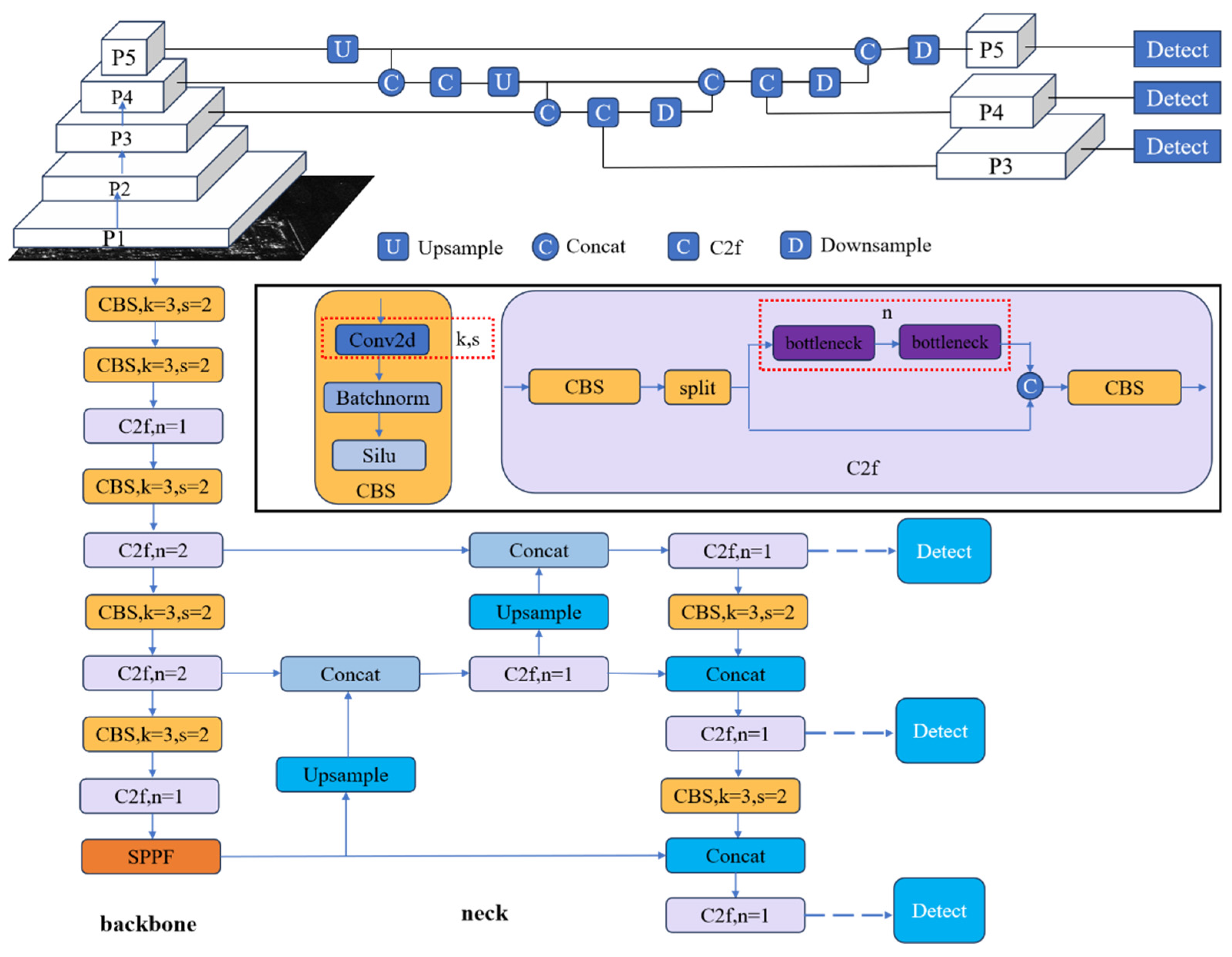
Figure 2.
Schematic of detection layer adjustment.
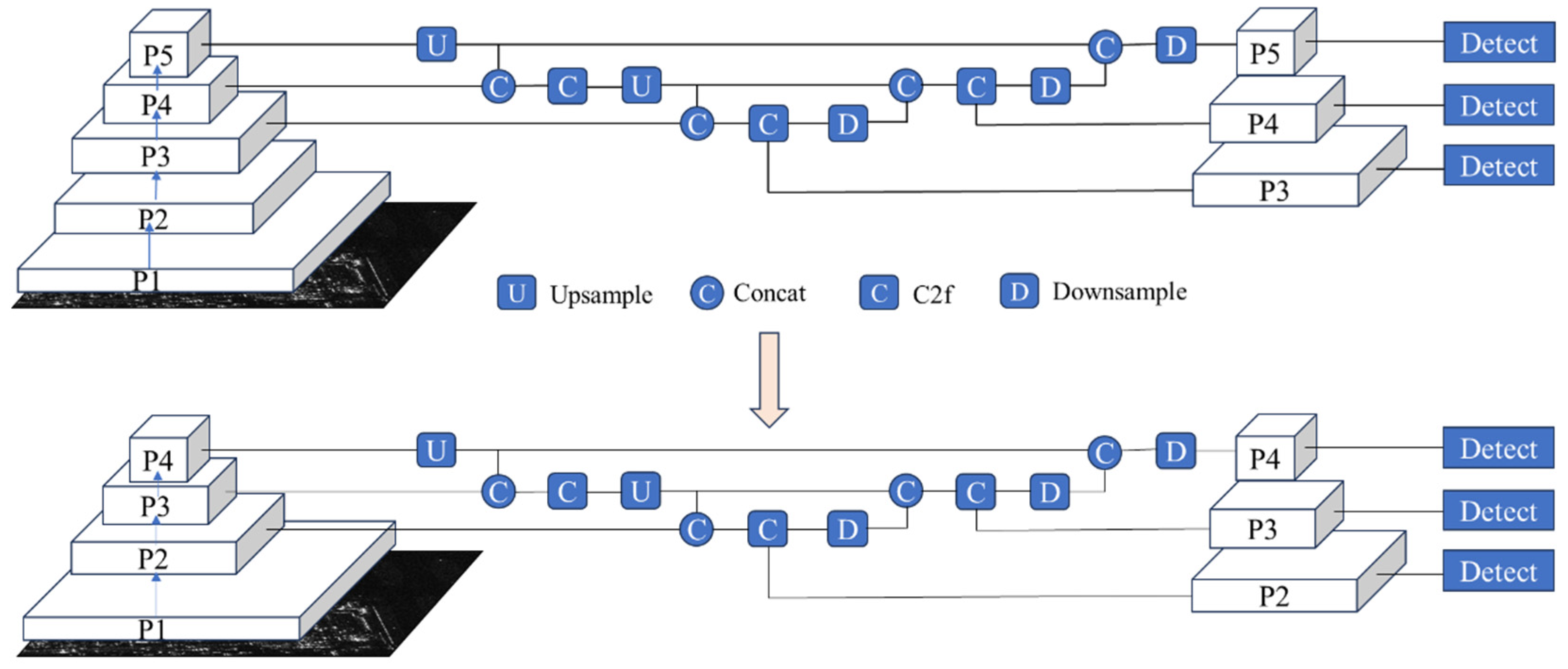
Figure 3.
Feature map downsampling methods. (a) The downsampling process using max pooling, (b) The downsampling process using strided convolution.
Figure 3.
Feature map downsampling methods. (a) The downsampling process using max pooling, (b) The downsampling process using strided convolution.
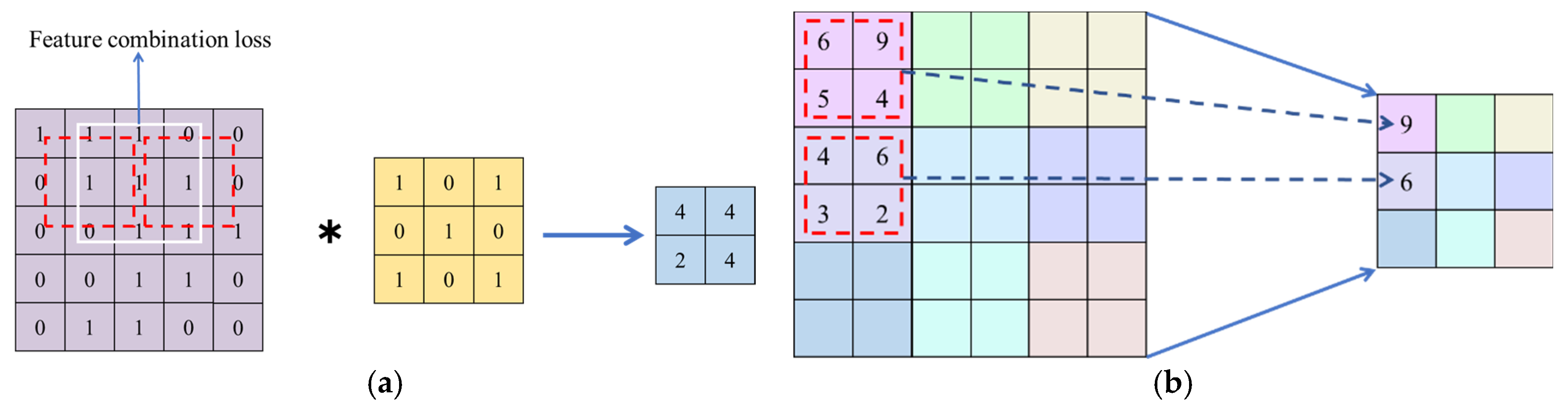
Figure 4.
Structure diagram of the Conv-Passthrough-DSC (CPD) module. The left shows the overall structure of the CPD module, and the right illustrates the passthrough operation.
Figure 4.
Structure diagram of the Conv-Passthrough-DSC (CPD) module. The left shows the overall structure of the CPD module, and the right illustrates the passthrough operation.
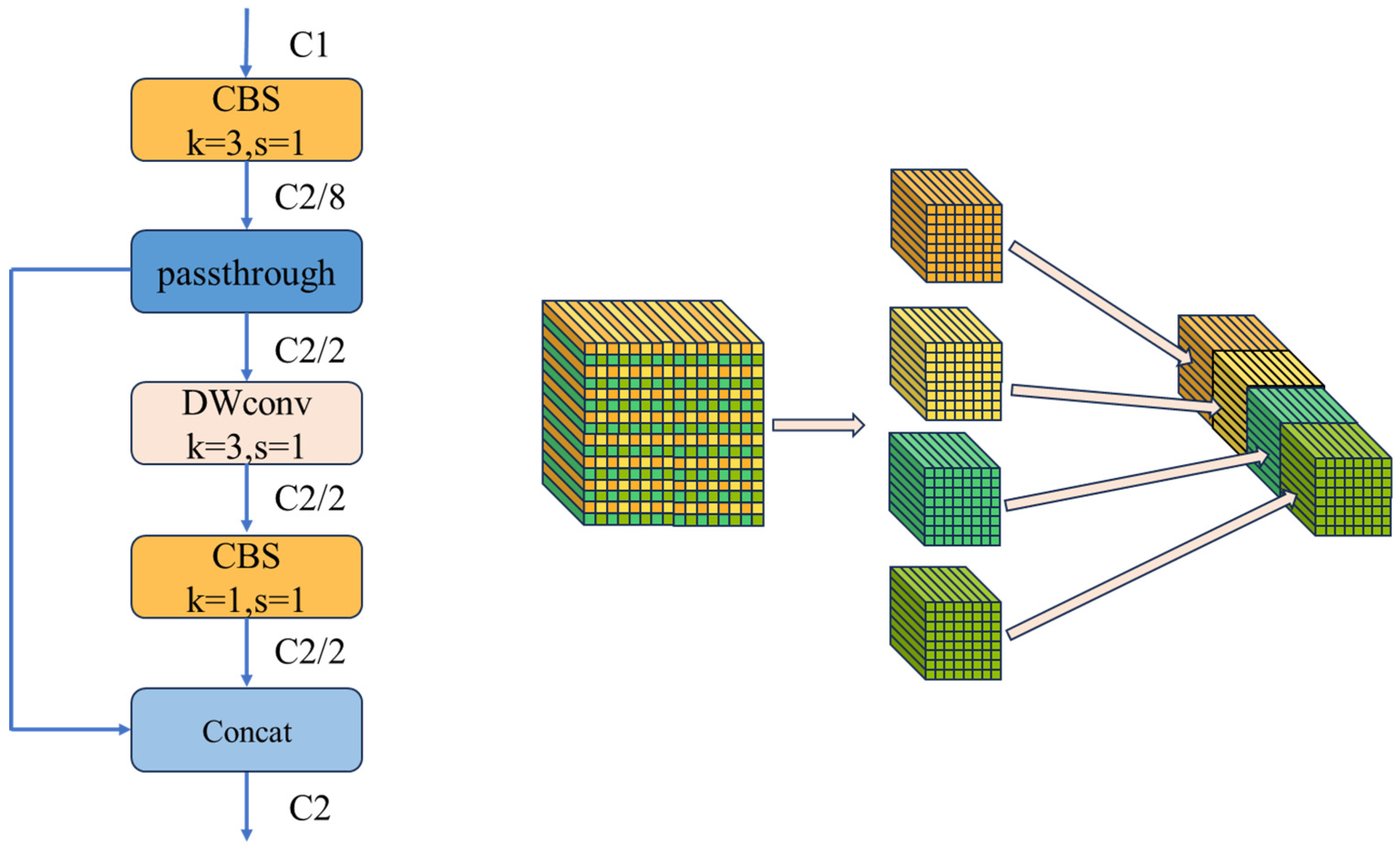
Figure 5.
Receptive field analysis. (a) Receptive field of the feature map after downsampling by a stride-2 convolution with a 3x3 kernel. (b) Receptive field of the feature map after downsampling by the CPD module.
Figure 5.
Receptive field analysis. (a) Receptive field of the feature map after downsampling by a stride-2 convolution with a 3x3 kernel. (b) Receptive field of the feature map after downsampling by the CPD module.
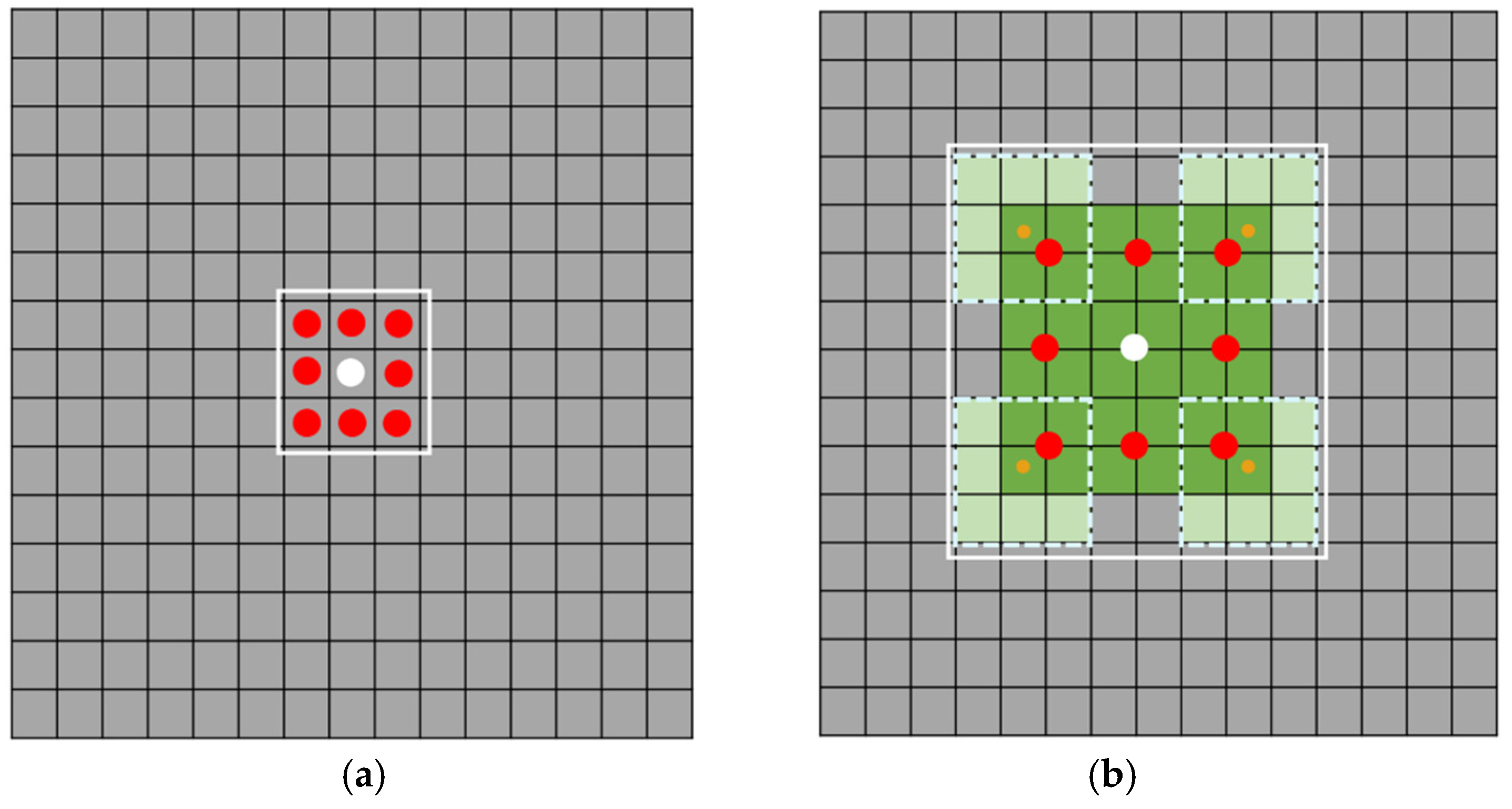
Figure 6.
Overall structure of the FCCS-YOLO network.
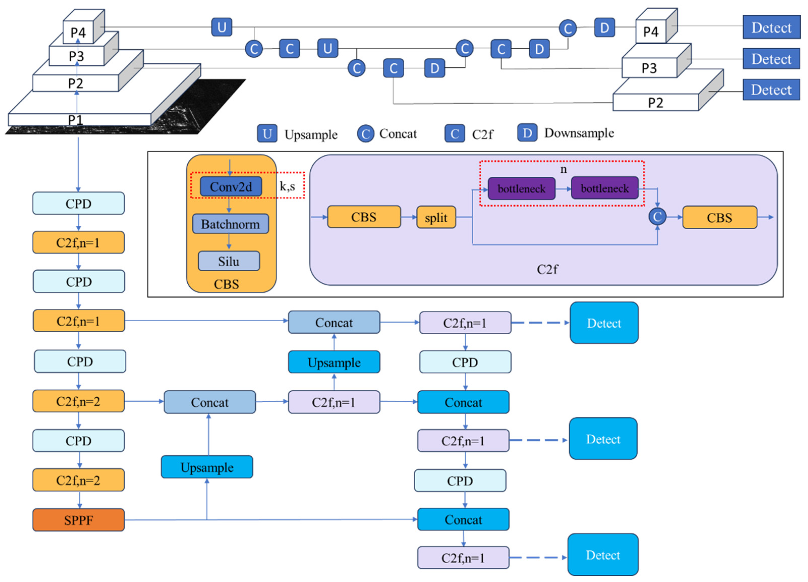
Figure 7.
Skew Intersection over Union (SIOU) Calculation Diagram.
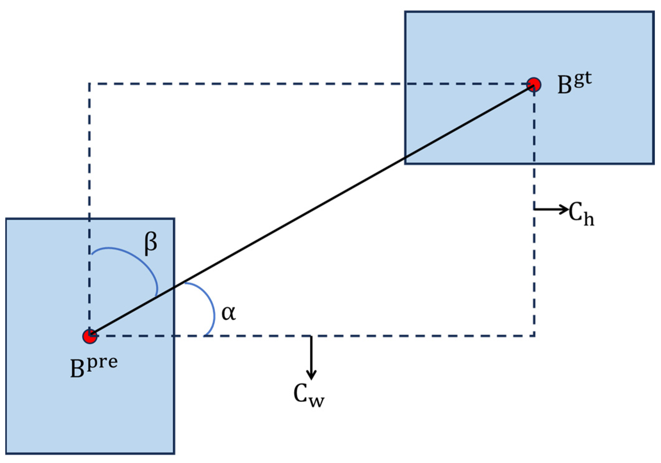
Figure 8.
Illustration of Positive and Negative Sample Sampling.
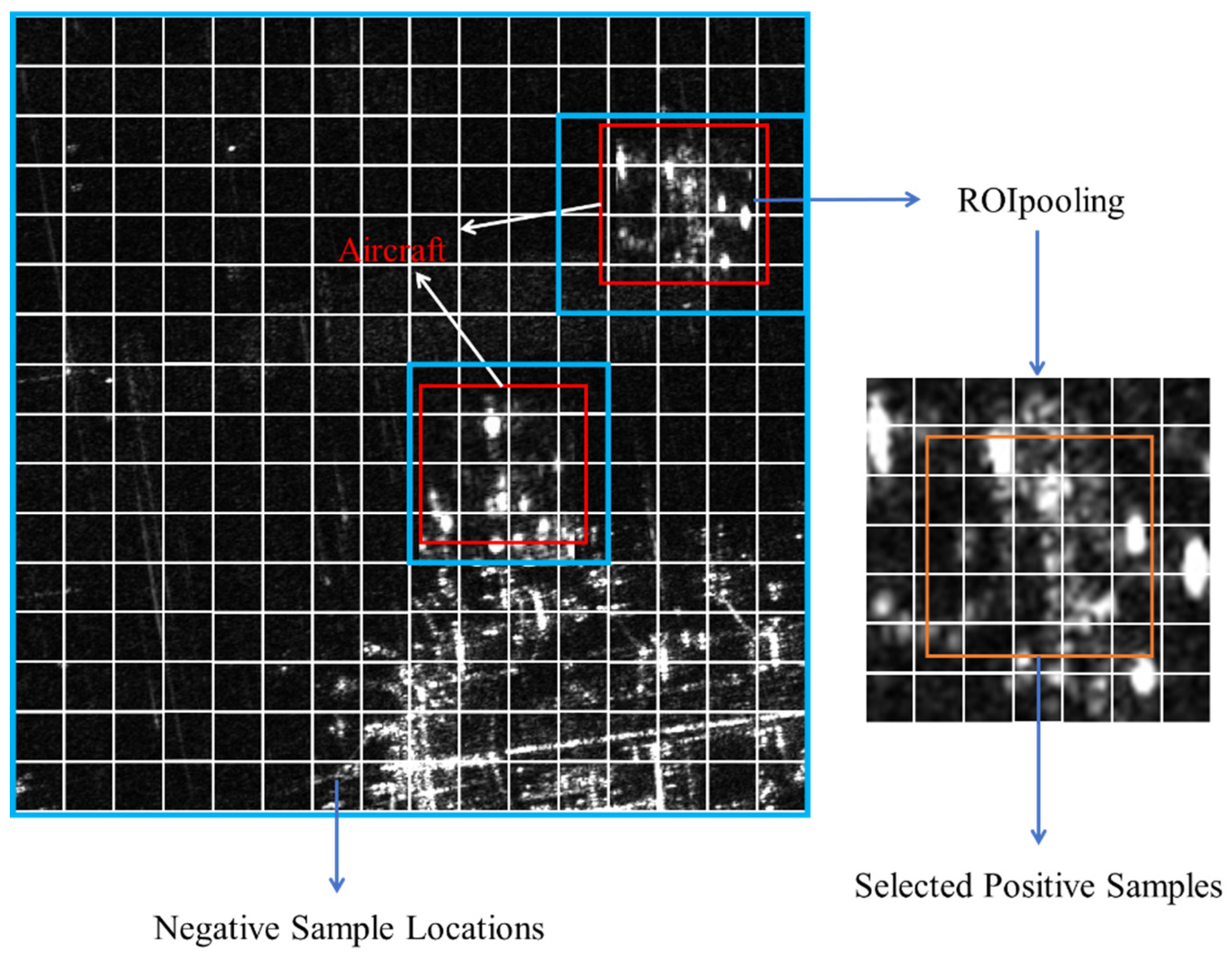
Figure 9.
The visual results on the SAR-AIRcraft-1.0 dataset are displayed. The first column represents the ground truth, the second column shows the detection results from Faster-RCNN, the third column presents the YOLOv8 detection results, and the fourth column displays the detection results from FCCS-YOLO.
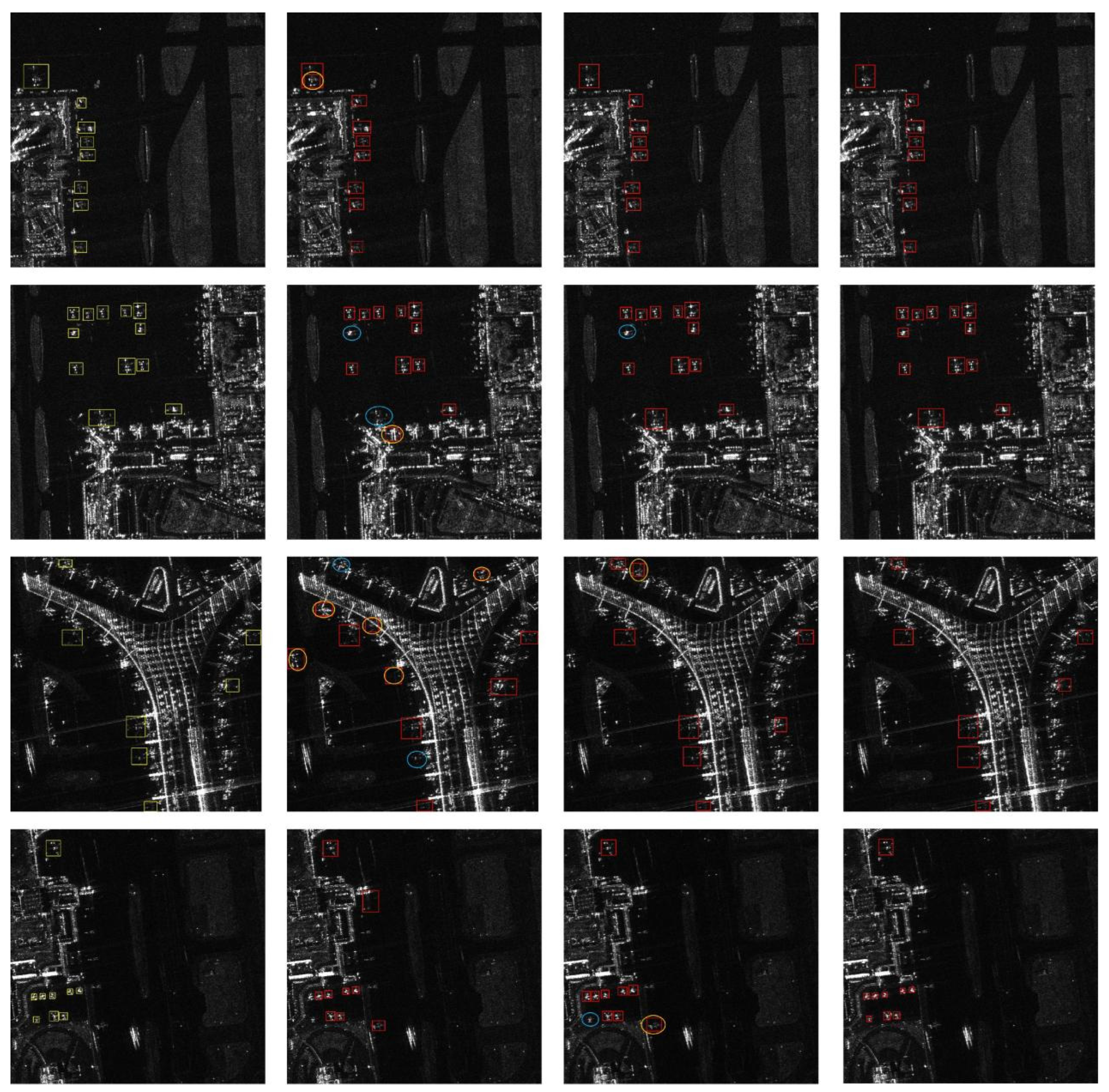
Figure 10.
Proportions of High-Confidence Predictions Across Feature Maps. (a) illustrates the distribution of high-confidence predictions across feature maps in the YOLOv8n, while (b) illustrates the distribution of high-confidence predictions across feature maps after modifying the detection layers.
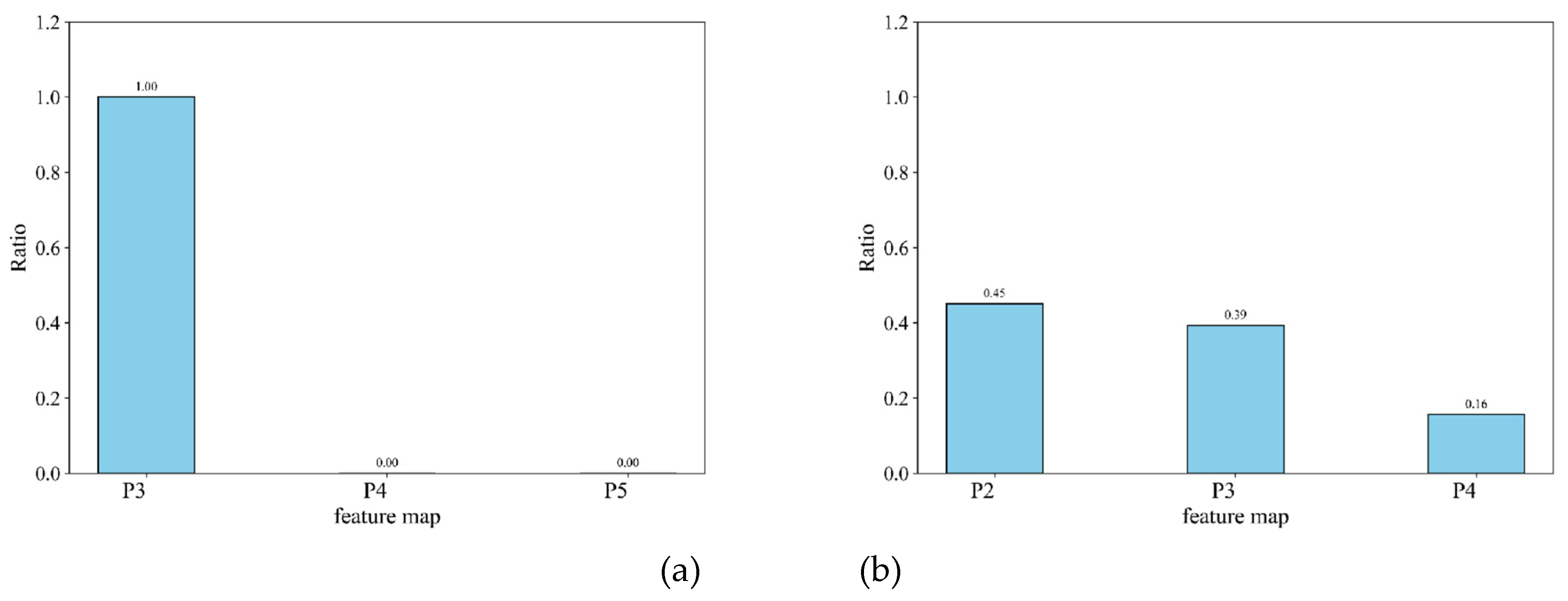
Figure 11.
Loss Curve During Training.

Figure 12.
The distance distribution of positive and negative samples relative to the average positive sample in the feature map.
Figure 12.
The distance distribution of positive and negative samples relative to the average positive sample in the feature map.
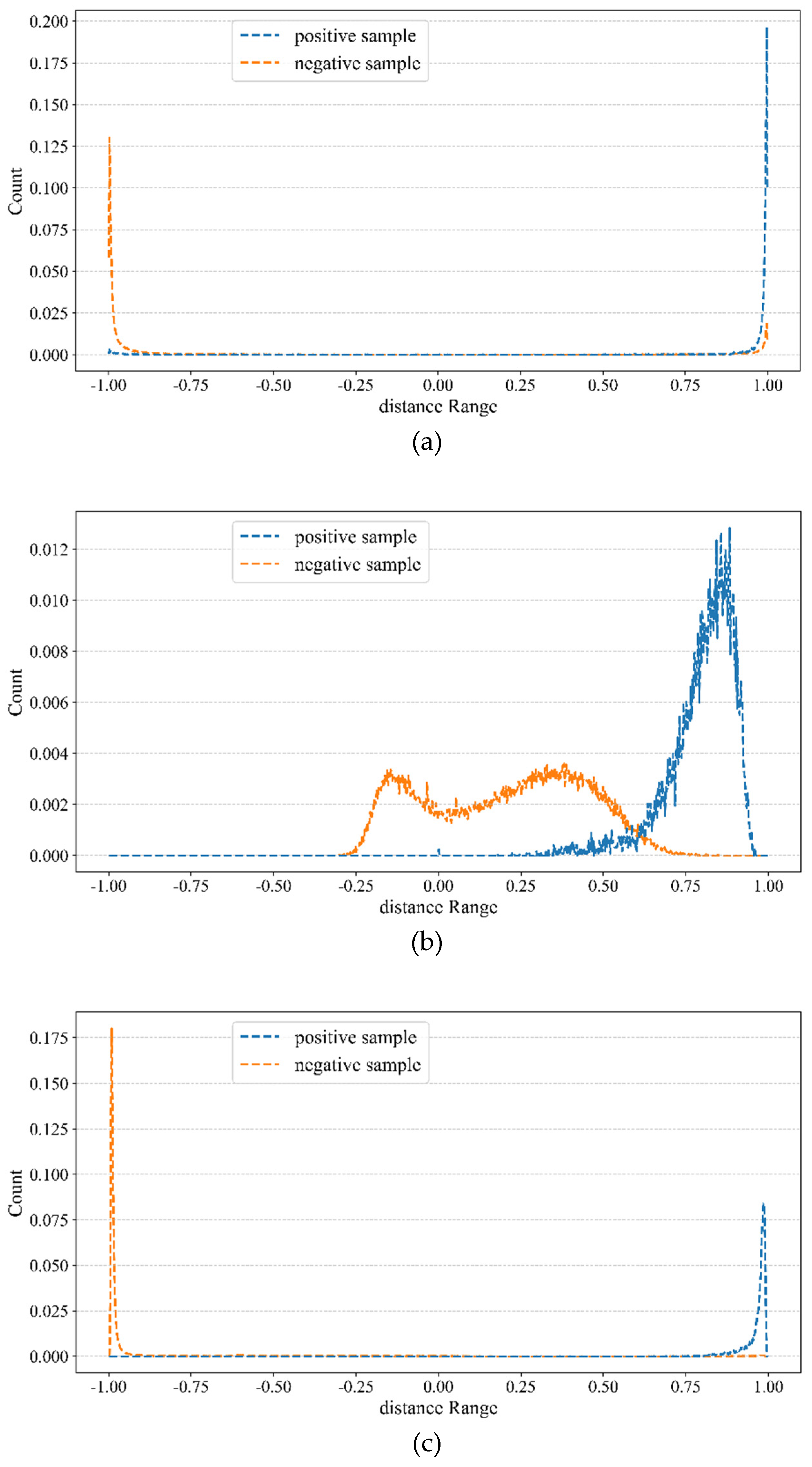

Table 1.
Ablation experiments.
| A | B | C | D | E | |
|---|---|---|---|---|---|
| layer adjustment | × | √ | √ | √ | √ |
| CPD | × | × | √ | √ | √ |
| SIOU | × | × | × | √ | √ |
| contrastive learning | × | × | × | × | √ |
| mAP50 (%) | 93.8 | 93.9 | 94.3 | 94.8 | 95.5 |
| P (%) | 86.3 | 85.5 | 86.5 | 87.1 | 90.0 |
| R (%) | 89.0 | 91.3 | 91.4 | 92.0 | 93.2 |
| Params (M) | 3.01 | 0.98 | 0.87 | 0.87 | 0.87 |
Table 2.
FCCS-YOLO versus other networks on the SAR-AIRcraft-1.0 dataset.
| Methods | mAP50 (%) | P (%) | R (%) | Params (M) |
|---|---|---|---|---|
| Faster R-CNN | 70.5 | 72.2 | 75.3 | 44.25 |
| Cascade R-CNN | 77.8 | 89.0 | 79.5 | 50.2 |
| SSD | 79.2 | 82.0 | 78.2 | 45 |
| FCOS | 87.0 | 76.5 | 80.6 | 34.5 |
| CenterNet | 90.9 | 82.3 | 82.1 | 34 |
| YOLOv5 | 92.1 | 87.3 | 83.6 | 4.53 |
| YOLOv8 | 93.8 | 86.3 | 89.0 | 3.01 |
| FCCS-YOLO | 95.5 | 90.1 | 93.2 | 0.87 |
Disclaimer/Publisher’s Note: The statements, opinions and data contained in all publications are solely those of the individual author(s) and contributor(s) and not of MDPI and/or the editor(s). MDPI and/or the editor(s) disclaim responsibility for any injury to people or property resulting from any ideas, methods, instructions or products referred to in the content. |
© 2024 by the authors. Licensee MDPI, Basel, Switzerland. This article is an open access article distributed under the terms and conditions of the Creative Commons Attribution (CC BY) license (https://creativecommons.org/licenses/by/4.0/).
Copyright: This open access article is published under a Creative Commons CC BY 4.0 license, which permit the free download, distribution, and reuse, provided that the author and preprint are cited in any reuse.


