
Submitted:
10 July 2025
Posted:
11 July 2025
You are already at the latest version
Abstract
In the following paper an optimization approach for the optimal design of tuned mass dampers in structural dynamics is presented. The approach considers uncertain system parameters and the tuned mass damper performance is measured by means of the total and relative displacements of the structure. In a first step, a single-degree-of-freedom system is investigated using an analytical formulation of the amplification function. The uncertainty propagation is implemented by an efficient linearization approach where each value of the amplification function is considered separately. The optimization goal functions are the minimization of the damper mass and the minimization of the maximum displacements by considering mean and standard deviation of the random system responses. The presented approach is extended for multi-degree-of-freedom systems by an efficient modal decomposition approach, which will be proven to be sufficiently accurate. By means of several examples, the overall robust design optimization procedure is discussed and different assumptions for the optimization goals and different optimization methods are investigated.
Keywords:
tuned mass damper
; stationary solution
; uncertainty quantification
; robust design optimization
; reduced order model
1. Introduction
The application of tuned mass dampers (TMD) for the reduction of structural vibrations is a well known procedure started with the early investigations by Den Hartog [1]. Typically, high-rise buildings under earth-quake and wind excitations require the TMD technology to reach new heights or to enable the construction under special loading conditions. An overview of existing famous buildings with TMD applications is given in [2]. Early studies for structures subjected to wind loads can be found in [3,4], as well as for earthquake excitations in [5,6].
From the mechanical viewpoint, the original structure is often simplified as an single-degree-of freedom (SDOF) system and the consideration of the TMD extends the system to a 2-DOF system. Early analytical investigations on the influence of the TMD parameters with respect to the structural vibrations can be found in [7] for harmonic and white noise excitation, and in [8,9,10], where different design criteria in the time and frequency domain have been investigated analytically. A good summary of optimal design criteria, with respect to maximum displacements or accelerations, vibration energy etc. is given in [11]. Recent investigations of this topic can be found in [12], where the maximum dynamical amplification is considered in the frequency domain via the frequency response functions.
Further extensions to more complex systems appeared later for multi-degree-of-freedom (MDOF) systems with single TMD [13] and SDOF systems with multiple TMDs [14,15]. In the most investigations, a white noise excitation or the maximum amplification were considered as design criteria.
With the availability of more general numerical optimization and machine learning methods, the optimal design of structures with single or multiple TMDs came into the focus of many investigations as summarized in [16,17]. Especially, the application of Particle Swarm optimization [18] and genetic algorithms [19,20] for MDOF structures with multiple TMDs enabled the automatized optimization of the TMD parameter as mass, stiffness and damping as well as an optimal number and optimal positions of the TMDs in an MDOF structure. Typical application examples are frame structures and slender bridges. With help of neural network approximation the parametric optimization of SDOF system optimization was generalized in [21,22].
Additional to the optimal tuning of the TMDs, the accurate knowledge of the main system properties as well as the TMD parameters are essential for an optimal performance of the TMDs. Therefore, the influence of uncertainties on the TMD performance and reliability is a critical issue. One early investigation on the influence of random input parameters for SDOF systems with stationary and non-stationary excitation was published in [23]. The application of Reliability-based Design and Robust Design Optimization methods summarized in [24] came into the focus for the optimal design of TMDs mainly in the last decade. In [25] an SDOF system plus TMD was investigated considering parametric uncertainty as random numbers. A stochastic excitation of an SDOF system with maximum displacements as performance criterion was optimized in [26]. In [27] a multi-objective optimization approach was presented, where the mean and the scatter of the performance measures were optimized simultaneously by a Pareto optimization approach. One recent application to the optimal design of footbridge can be found in [28]. Multiple TMDs applied to an SDOF system have been investigated in [29,30], whereby the displacement solution of the equation of motion was obtained by a numerical time integration using the Newmark method. Since a coupled Robust Design Optimization would require the evaluation of the statistical performance measure for every design parameter combination, the time integration might be the critical bottle-neck in the numerical analysis. Therefor, approximation methods have been introduced recently for the optimal design of TMDs considering uncertainties. A straight-forward Kriging approximation is considered in [31] and a linearization approach is presented in [32].
In the following study, first the performance of a TMD attached to an SDOF system is evaluated by means of the dynamic amplification function based on the analytical solution given in [9]. The robustness of the TMD is assessed by a variance-based approach considering the safety margin of the maximum amplification function value. In contrast to the reliability analysis, no definition of a limit state is necessary, we just introduce the required safety level from the definitions in the design code. In a further step, a perturbation approach is utilized to simplify the uncertainty propagation problem. We will show, that the linearization of the performance measure or objective itself, as introduced in [32], is not sufficiently accurate and therefor the linearization is applied for the individual values of the amplification function. Additionally, the choice of the design parameters for the optimization and the scattering inputs for the uncertainty analysis is very important and will be discussed in detail.
An efficient extension for MDOF systems with multiple TMDs is introduced by a modal decomposition of the main system and a decoupled analysis of the individual TMD amplifications. We will prove a sufficient accuracy of this reduced order model by a comparisson with numerical time integration methods. The decoupled stationary solution can provide the maximum displacement solution for all DOFs of the system very efficiently and could be used to consider the maximum amplification as optimization objective similar to SDOF systems. Additionally, we will show, that the linearization approach performs quite well for this type of reduced order model. Additionally to the estimates of the displacement uncertainty of all DOFs, the proposed algorithmic framework offers a very fast estimate of variance-based sensitivity measures, which could help to identify most relevant sources of uncertainty and possibly improve the knowledge of the uncertainty of the input parameters. All together, the presented approach enables an efficient optimization of the TMD parameters under the consideration of uncertainties.
2. Materials and Methods
2.1. Single-Degree-of-Freedom Systems
In the following section, we assume an SDOF system, which could be a simplified mechanical beam model of a pedestrian bridge as shown in Figure 1.
If only a single natural mode of vibration is considered in the analysis, the main system can be modeled as single-degree-of-freedom (SDOF) system with the following equation of motion [34]
Assuming a harmonic excitation
where is the force amplitude and the circular frequency of the excitation, the particular (stationary) displacement solution for the equation of motion reads [9]
with
The natural circular frequency of the undamped system and the damping ratio is given as
A performance measure within the design process can be the maximum value of the dynamic amplification function , as it amplifies the ratio of force amplitude and system stiffness in the resonance case. Figure 2 shows an example of the amplification function assuming a damping ratio of .
If a tuned mass damper (TMD) is taken into account as the second degree of freedom, as shown in Figure 1, the following equations of motion are obtained
where describes the relative displacement between the main system and the tuned mass damper. Introducing and as
the equations of motion read
Assuming a harmonic excitation, the stationary displacements result analogously [9] to
with the dynamic amplification functions
and
Decisive parameters in the tuning of the TMD are the mass ratio , the frequency ratio and the damping rate of the attached vibration damper. The natural circular frequencies of the undamped 2-DOF system can be obtained as follows [35]
with the corresponding frequency ratios
2.2. Optimal Tuning of the TMD Parameters
The optimal parameters of a vibration damper with deterministic properties are usually formulated as a function of the mass ratio [9]. The optimal parameters for minimum displacements are given according to Den Hartog as
In Figure 2, the amplification functions from Equation (10) for the displacements of the main system and for the relative displacements are shown for different mass ratios. The figure indicates, that the maximum values of both amplification functions decrease with increasing mass ratio.
Alternatively to the Den Hartog formulas, the optimal values can be obtained by mathematical optimization. If the maximum value of the dynamic amplification function of the main system should be minimized for a given maximum mass ratio , the optimization task can be defined as a single-objective optimization problem as follows
Since an increase of the mass ratio always decreases the amplification function values, the mass ratio can be considered constant as the limit value and the frequency ratio and the damping rate can be considered as the remaining optimization variables.
As optimization algorithms gradient-based approaches as Quasi-Newton methods [36] as well as gradient-free methods can be applied without special adjustments. In this study an extended Nelder-Mead method is used [37], which is very efficient for a small number of optimization variables. The advantage of an optimization approach compared to the analytical formulas according to Den Hartog and others [9], is that additional constraints such as the maximum relative displacement between main system and the TMD can be considered in a straight forward manner. In the first example in Section 3.1, the amplification function obtained with the optimum parameters according to Den Hartog is compared to the results of a single-objective optimization. For this purpose, different formulations of the objective function are investigated.
However, if we want to minimize the mass ratio of the vibration damper and the maximum values of the amplification function simultaneously, the optimization task can be solved either by gradually adjusting the limit for the mass ratio within a single-objective problem or as a multi-objective problem using Pareto optimization. The objective functions can be formulated as follows
where , and are the optimization variables. In case of conflicting objectives, no unique optimal solution exists and the optimal designs build a so-called Pareto-frontier as shown in Figure 3. In our study, we use the Non-dominated Sort Genetic Algorithm (NSGA II) according to [38] as Pareto optimization algorithm. This algorithm uses a sorting of the Pareto dominance as performance criterion as shown additionally in Figure 3. In Section 3.1 the results of the Pareto optimization are investigated in detail for an SDOF system.
2.3. Uncertainty Propagation and Quantification
When analyzing the propagation of uncertainty, it is advisable to assume the basic variables of the system as scattering variables, as the scattering can usually be determined directly for these variables. This means, that the mass and stiffness coefficients as well as the damping ratios of the main system and the TMD are considered as random numbers, which could be summarized in a random vector
Each random number can be defined as a scalar random variable by a distribution function and statistical moments such as mean value and standard deviation. The values of the amplification functions for discrete values of the excitation frequency ratio can be represented as scalar random numbers as well
The statistical properties of the amplification function values can be investigated by sampling methods such as the Monte Carlo Simulation [39], where a certain number of random samples is generated according to the defined distribution of the input parameters. Correlations between the inputs could be considered by the Nataf model [40]. Further details on sampling approaches and correlation models can be found in [41]. In our study, an improved Latin Hypercube sampling (LHS) according to [42] is applied, where the marginal distributions are represented with respect to the probability contribution and spurious correlations between the inputs are minimized as shown in Figure 4.
The statistical properties of the amplification function values could be analyzed by histograms and the estimates of statistical moments. Additional to the properties of a single output, the dependence with respect to the random input parameters might be interesting. A quite common approach for such a sensitivity analysis is the global variance-based method. In this method, the contribution of the variation of the input parameters with respect to the variation of a certain model output is analyzed. The variance contribution of the parameter with respect to a model output can be quantified with the first order sensitivity measure introduced by [43]
where is the unconditional variance of and is called the variance of conditional expectation with denoting the set of all parameters but . Furthermore, measures the first order effect of on the model output. Since first order sensitivity indices quantify only the decoupled influence of each parameter, the total effect sensitivity indices have been introduced by [44] as follows
where measures the first order effect of on the model output which does not contain any effect corresponding to .
Generally, the computation of and requires special estimators with a large number of model evaluations [45]. In [41] regression based estimators have been introduced, which require only a single sample set of the model input parameters and the corresponding model outputs. Based on a linear or quadratic regression model, the so-called Coefficient of Importance (CoI) is evaluated. With the Metamodel of Optimal Prognosis (MOP) [46] a more general meta-model based approach for variance-based sensitivity analysis was introduced, where the quality of the meta-model is estimated with the Coefficient of Prognosis (CoP) by means of a sample cross-validation. In the MOP approach, different types of meta-models such as classical response surface models [47], Kriging [48], Moving Least Squares [49] as well as artificial neural networks [50] are tested automatically for a specific model output and evaluated by means of the CoP measure. This approach is available with the Ansys optiSLang software package [51]. Further information on the CoP measure can be found in [52]. An extension of the variance-based sensitivity measures for correlated inputs was introduced in [53].
Since the scatter of the random response values, e.g. the maximum amplification function value, for a given nominal design of the input parameters should be considered in an outer optimization loop, the sampling based estimation of the response scatter might be numerically demanding. Therefor, another much more efficient approach is investigated in this study: If the individual amplification function values will be linearized w.r.t. the random input parameters using a Taylor series expansion at the nominal values, the mean values and the variance of the linearized response values can be estimated in closed form without any assumption on the input parameter distributions. By assuming the optimal deterministic parameter values as mean values
the random amplification function values in Equation (18) can be linearized as follows
Based on this linearization, the mean value and the variance of each amplification function value can be obtained from the standard deviation and the correlation coefficients of the p random inputs as follows
The required derivatives in Equation (22) could be obtained by the central difference method. In case of uncorrelated inputs, Equation (23) simplifies as follows
and the sensitivity indices can be estimated as
2.4. Optimization Under Uncertainty
By considering uncertain input parameters in the optimization task, we have to distinguish between purely random inputs and design variables, which could be random as well [24]. Let us consider the design variables for the SDOF-system similarly as within the deterministic optimization as the nominal values of , and
The corresponding random numbers for the TMD coefficients are
where the mean values are adapted by the design variables
The standard deviation of each parameter could be assumed either as a constant value or could be obtained from the current mean value and a given Coefficient of Variation (CoV)
The statistical properties of the pure random parameters of the main system
remain constant during the optimization.
In Reliability-based Design Optimization, the objective function is usually formulated in terms of the deterministic design variables . Statistical constraints are introduced to consider certain quality requirements [24]
where are limit state functions depending on the joint set of and and is the corresponding failure probability, which must not exceed a given target value. In Figure 5 a single random response Y is shown with an indicated limit .
The limit state function can be formulated in this case as follows
The evaluation of the failure probability requires an integration of the joint probability density function over the failure domain
which might be numerically very demanding for the general case [41].
Within the Design-for-Six-Sigma approach, the optimization constraints are typically formulated in terms of the safety margin of the random output [54]
which is usually formulated by the standard deviation times a required sigma level . Different procedures for this so-called Robust Design Optimization (RDO) are discussed in [55] and more recently in [24]. Typically, a double loop approach is necessary, where the outer loop performs the optimization and an inner loop estimates the output mean values and standard deviations with respect to the current nominal values of the design variables.
For the optimization of the TMD parameters, we will apply the linearization approach to estimate the mean value and the standard deviation of the individual amplification function values and . If a certain limit for the dynamic amplification is given, the optimization task can be formulated in terms of a minimization of the nominal TMD mass ratio as follows
where the constraints could be formulated alternatively in terms of the maximum displacements by using Equation (9). If no limit values for the amplification function or displacements are defined, we could either minimize the mass ratio and the maximum amplification values within a multi-objective optimization
or the mass ratio could be kept fixed and the maximum amplification values are minimized. The scaling factor , which defines the safety margin in terms of the standard deviation, is chosen in this study according to the probability levels for the serviceability limit state and the ultimate limit state according to the European design code [56].
2.5. Extension for Multi-Degree-of-Freedom-Systems
The equation of motion for a linear multi-degree-of-freedom (MDOF) system reads in matrix-vector notation as follows
where the mass matrix , the damping matrix and the stiffness matrix correspond to an initial main system without TMD. For the free vibration mode of the undamped system, the natural circular frequencies and the corresponding mode shapes can be obtained by solving the following eigenvalue problem
Since the eigen-modes are orthogonal to each other
the equations of motion could be decoupled in case of a modal damping [35]
whereby the displacement solution in the n original degrees of freedom can be obtained by a superposition of the decoupled modal solutions.
If we extend the MDOF-system by several tuned mass dampers, which are coupled directly to certain degrees of freedom of the initial main system, we get a coupled damping and stiffness matrix in the equation of motion
where , , and as well as , , and are sub-matrices which represent the damping and stiffness coefficients of the tuned mass dampers and their association to the coupled degrees of freedom of the main system. If an optimization is applied to obtain optimal TMD coefficients, the corresponding damping and stiffness coefficients could be varied independently of each other. A specific modal damping matrix, which could be decoupled similarly as for the main system itself, could not be obtained in the standard case. Therefor, time integration methods as the Newmark-Beta approach [35] are necessary to solve Equation (42). However, this procedure is very demanding from the computational point of view. Especially, if the maximum amplification function of a certain degree of freedom should be considered in the objective function, a sweep over the excitation frequency has to be considered.
In order to decrease the numerical effort, we assume a decoupled influence of each TMD by designing it only for a single vibration mode of the main system. For example, if we would assume a tuning for the first mode shape, we would approximate the displacement solution as the super position of a 2-DOF-system for the first mode and several SDOF-systems for the higher modes as illustrated in Figure 6.
The stationary displacements of the original DOFs can be assembled for this assumption as follows
where the decoupled solution of an individual vibration mode reads in case of an application of a TMD
The modal stiffness corresponds to the main system and the force amplitudes result from a harmonic excitation as follows
The amplification function and the phase shift have to consider the modal mass and damping as well as the corresponding undamped circular frequency of the main system for the calculation according to Equation (9)
The corresponding mode shape has to be normalized with respect to the DOF, where the TMD is applied. For the other vibration modes, where no TMD is applied, the decoupled stationary displacement solution reads
where and are the amplification function and the phase shift of a standard SDOF system according to Equation (4)
The maximum stationary displacements of the orginal DOFs can be obtained from the assembled stationary displacements according to Equation (43) for one vibration period while considering the individual phase shifts in Equation (44) and Equation (47). The relative displacements of TMDs with respect to the coupling DOFs result for the decoupled stationary solution similar as for the main system as
with
In the second example, we will show, that the approximated displacement solution agrees very well with the results from a time integration and can be used to estimate the maximum displacements for the full excitation frequency range very efficiently.
For the uncertainty quantification, we introduce the maximum displacements of the original DOFs and maximum relative displacements of the TMDs for a given excitation frequency as scalar random outputs
where the linearization approach with respect to the random input vector can be applied similarly as for the SDOF system
The variance of these outputs and the sensitivity indices with respect to the random inputs can be directly estimated using Equation (24) and (25). The random input vector contains the random inputs of the main system , which define the scatter of the MDOF system itself, and the random properties of the m TMDs
As design variables within the Robust Design Optimization, we consider the nominal values of the mass ratio , the nominal circular frequencies and the nominal damping ratio of each TMD
The choice of design variables is based on the investigations in [57] and is more suitable as the basic mass, stiffness and damping coefficients in the equation of motion.
The objective functions within the Robust Design Optimization are defined similarly as for the SDOF system, but the total mass of all TMDs and the safety margin of specific displacements of the main system could be considered
Additional constraints with respect to the TMDs relative displacements could be formulated in a straight-forward manner.
3. Results
3.1. Single-Degree-of-Freedom Example
3.1.1. Deterministic Optimization
In the first example we investigated an SDOF system with a TMD as shown in Figure 1. The parameters for the main system have been chosen exemplarily and are given in Table 1. Additionally, the optimal parameters according to Den Hartog are given for a mass ratio of . In a first step we performed a single-objective optimization with the objective function
for a fixed mass ratio of . The parameter bounds for the optimization variables and are given in Table 1. In Figure 7 the function of the maximum value of is shown within the parameter bounds. The figure clearly indicates an unimodal objective function with a single optimum. As optimization algorithm the simplex method [37] from the Ansys optiSLang software package [51] was utilized. The optimizer converged within 55 model evaluations. The parameter values of the optimal design agree very well with the optimal values according to Den Hartog as shown in Table 1. The corresponding amplification functions drawn in Figure 8 show a very good agreement.
In a second step, we investigated a different objective function by considering the amplification value at the resonance frequency only
The obtained amplification function is shown additionally in Figure 7 and Figure 8. As indicated in the second figure, the optimized SDOF+TMD system has two significant resonances which have an amplification close to the original SDOF system. Thus, a different excitation frequency would lead to similar displacements as without TMD. Even the relative displacements of the TMD w.r.t. the main system would be very large compared to the values obtained with the Den Hartog parameters. From this findings, we can summarize, that the consideration of a single specific excitation frequency might not lead to optimal amplification functions. Therefor, we consider the maximum amplification function as an objective in the following investigations.
In the next step, a multi-objective optimization was performed with the two objectives
by considering the parameter bounds given in Table 1. The NSGA-II method [38] of the Ansys optiSLang software package was used with 50 generations each having a population size of 50 in order to assure a good convergence. Figure 9 compares the resulting Pareto front of both objective functions and the results of several single-objective optimization runs with the optimal values according to Den Hartog. The relationship between the optimal mass ratio and the corresponding values of the frequency ratio and the damping ratio is particularly interesting. The scatter in the parameter values results from the stochastic nature of the NSGA-II. The optimal damping ratio according to Den Hartog is visibly lower than that of the optimizations, whereby the maximum values of the magnification functions hardly differ. As a result of the multi-objective optimization, a suitable choice for the mass ratio could be made: the range of about 2% to 5% mass ratio represents a good compromise between the conflicting objective functions. The relationship between the maximum values of the relative displacement is analogous to that of the main system. However, a limitation of the installation space and thus of the maximum displacements could be considered directly as a constraint in the single-objective and multi-objective optimization.
3.1.2. Uncertainty Quantification
In the next step, uncertain input parameters have been investigated. The input parameters were assumed to be independent and normally distributed as given in Table 2. The mean values were assumed as the optimal Den Hartog parameters for a mass ratio of 2% as given in Table 1. First, an improved Latin-Hypecube Sampling [42] with 1000 samples was generated and the corresponding amplification functions for each sample have been calculated. Figure 10 shows the first 100 samples which indicate a significant scattering of the magnification function in the range of the two maximum values corresponding to the natural frequencies.
The maximum amplification value and the amplification values and at the two natural frequencies and have been investigated in more detail. In Figure 11 the response values of the 1000 samples including the optimal approximation model by using the MOP are given with respect to the two most important inputs. The figure indicates a significant nonlinear function for the maximum amplification function value and a slightly nonlinear dependence for and . Furthermore, the figure shows the sensitivity indices based on linear and quadratic regression models and by using the more sophisticated MOP approximation. For and the linear and quadratic regression gives already suitable estimates and the explained variation of the full model is sufficient.
For all three outputs, the scatter of the stiffness values is indicated to be most dominant and the input scatter of the damping ratio seems minor important w.r.t. the response variation. However, the linear model can not explain the dependency for the maximum amplification value. For that reason, the linearization as introduced in Section 2.3 was applied directly for the individual amplification function values and not for the objective function itself.
In Figure 12 the estimated mean value and standard deviation of the amplification values are shown for the 1000 samples and for the linearization approach. In the figure a very good agreement could be observed, which indicates a sufficient representation of the scatter of the individual values and by the linearization. The derivatives required in Equation (22) have been estimated using the central difference method, which required only 12 model calls for the 6 input parameters. The corresponding derivation interval has been chosen as of the nominal parameter values. Additionally, Figure 12 shows the linearized variance contribution of the input parameters for the individual amplification values as introduced in Equation (24). Similar to the results in Figure 11, the scatter of the stiffness values seems most important for the values with the maximum scatter.
3.1.3. Optimization Under Uncertainty
Finally, the TMD for the SDOF system was optimized considering uncertain input parameters. As objective function, Equation (36) was considered, whereas the nominal values of and were taken as optimization variables and the nominal mass ratio was kept as . The input scatter was defined by the Coefficients of Variation given in Table 2. The mean values and the standard deviation of the individual amplification function values were estimated by the linearization approach. Figure 13 shows the corresponding maximum values of the mean and standard deviation as a function of the nominal values of and . The figure indicates, that a decreasing standard deviation correlates with an increasing mean value. Thus, a combination of both measures forms a compromise between nominal outputs and the scatter of the results. Similar to the deterministic case, the optimization was performed with the simplex method [37] from Ansys optiSLang. The -factor for the standard deviation in Equation (36) was assumed with and . Figure 13 shows the optimal values obtained for both cases in comparison to the deterministic solution. It is clearly recognizable, that for a higher weighting of the scattering, the optimal parameters tend towards higher damping values.
The amplification function values from the deterministic optimization and the optimum are compared in Figure 14, where the mean value curves and the mean values + 4.7 times the standard deviation are plotted. The figure clearly indicates an increased maximum mean value of the optimum compared to the deterministic solution, but the scatter is significantly smaller and thus a reduction of the statistical limit is possible.
As final investigation for the SDOF example, the single-objective robust design optimization was performed for different nominal values of the mass ratio and different safety margins by using again the simplex method. In Figure 15 the obtained maximum values for the mean and standard deviation as well as the corresponding nominal values for and are shown, whereby for , the nominal values correspond to the deterministic solution presented in Section 3.1.1. The figure indicates, that with increasing safety margin, the mean values increase but the standard deviation decreases. Furthermore, the damping ratio increases. This effect is most dominant for small mass ratios, where the influence of the uncertain input parameters is most critical.
3.2. Multi-Degree-of-Freedom Example with Single Tuned Mass Damper
3.2.1. Deterministic Analysis
In the second example, a multi-degree-of-freedom system as shown in Figure 16 was investigated. The deterministic values for the stiffnesses, masses and damping ratios have been taken according to the mean values in Table 3. The damping was assumed as modal damping as explained in Section 2.5. The three natural circular frequencies of the main system are , and . The corresponding amplification functions for a harmonic excitation are plotted in Figure 18. The peak values decrease for the larger natural frequencies due to the higher damping ratios. The TMDs have been designed for the first and second vibration mode and are coupled to the DOFs having the maximum value of the mode shape. Both mode shapes and were normalized with respect to the coupling DOFs and as shown in Figure 17, which results in the modal masses of . The optimal parameters for the nominal mass of the TMDs are taken according to Den Hartog as , and , which results in the nominal stiffnesses given in Table 3. The corresponding amplification functions for the first and second modes including the TMDs are shown additionally in Figure 18.
Figure 16.
MDOF example with 3 main DOFs and 2 TMDs
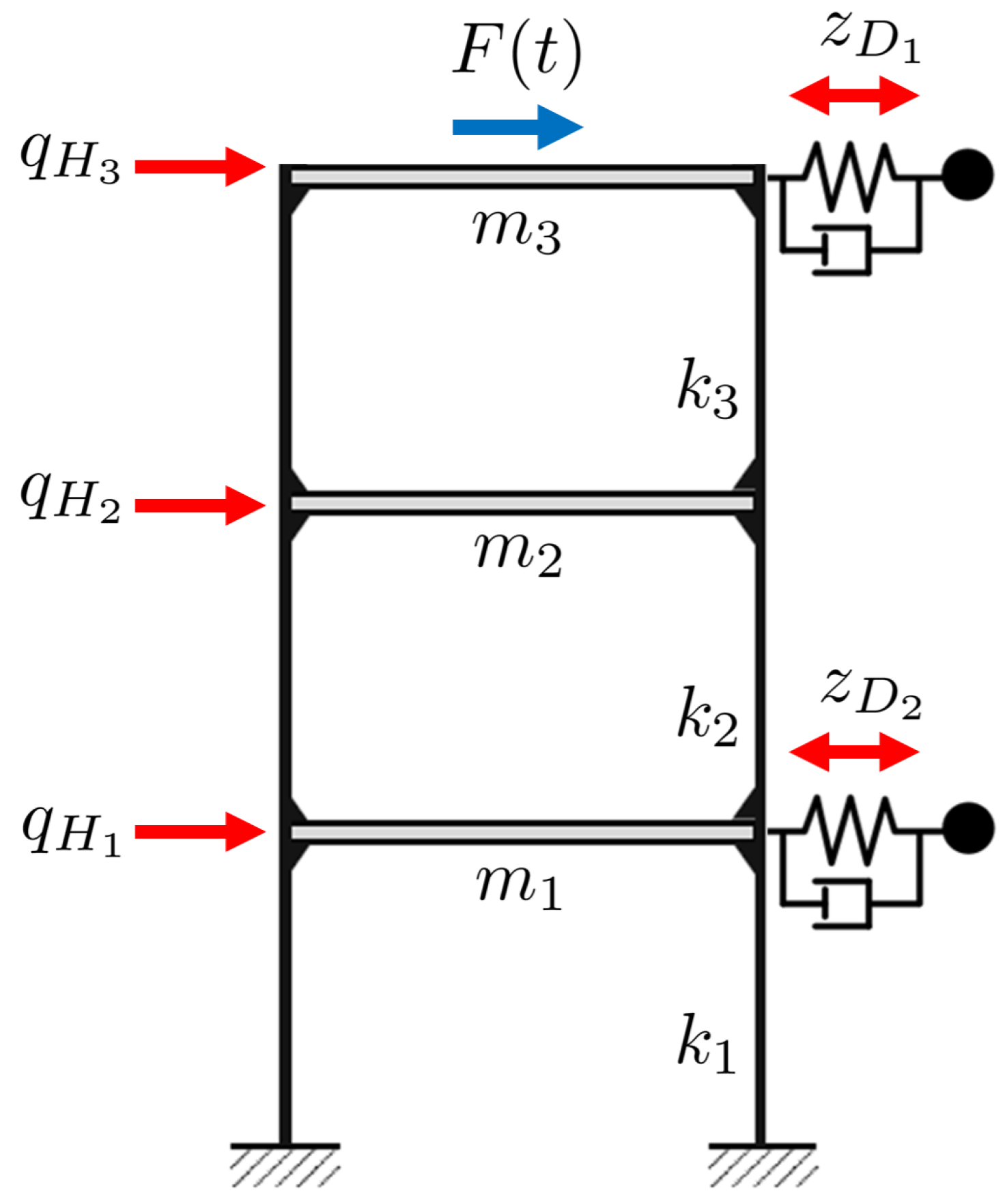
Figure 17.
Mode shapes of the initial 3-DOF system with , and
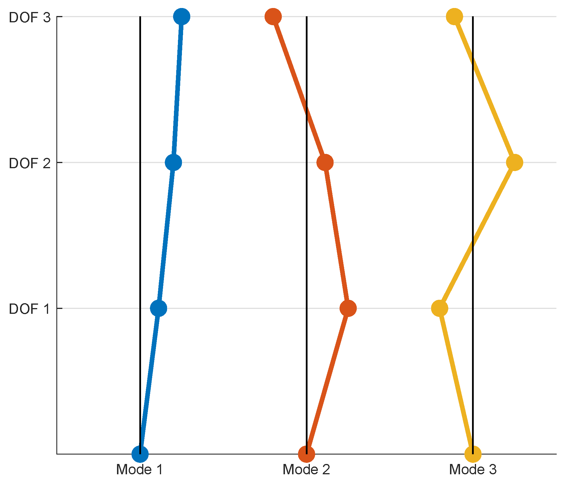
Figure 18.
Amplification functions for the 3-DOF system with and without TMDs (left) and approximated stationary displacements for an excitation frequency of (right)
Figure 18.
Amplification functions for the 3-DOF system with and without TMDs (left) and approximated stationary displacements for an excitation frequency of (right)
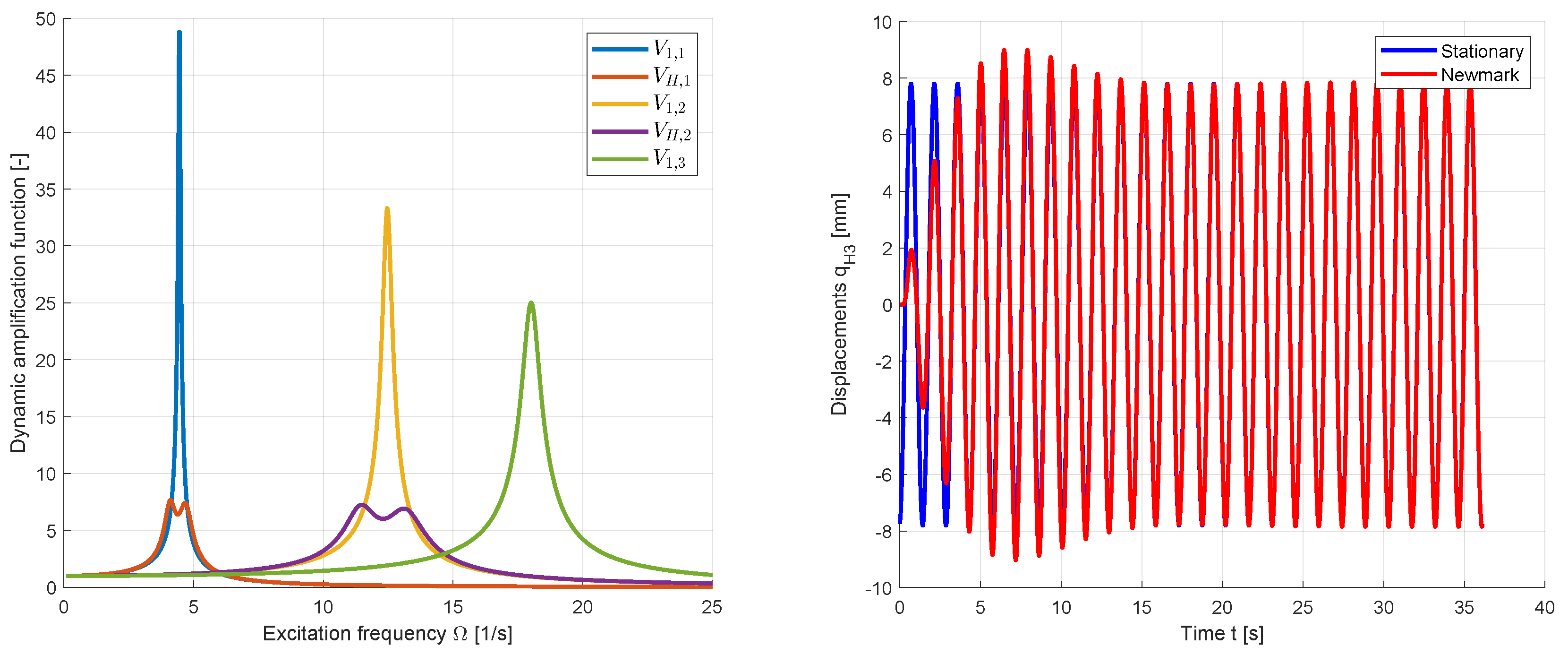
In a first step, the accuracy of the approximated displacement solution using the decoupled stationary approach according to Equation (43) was investigated. A harmonic excitation at DOF was assumed as . As benchmark method, the Newmark time integration was used for the full 5-DOF system including the TMDs within a time range of 100 excitation periods and a time step of of the smallest free vibration period of the initial main system. Figure 18 shows the displacements of DOF for the first 25 excitation periods with . The figure indicates a very good agreement of the approximated stationary solution with the Newmark results in the steady state. This analysis was repeated for different excitation frequencies and the maximum amplitudes of the Newmark results have been extracted from the last 25 excitation periods. In Figure 19 the vibration amplitudes in the steady state are compared for the displacements of all DOFs of the main system as well as for the relative displacements and of the TMDs. Additionally, the maximum values of the drift displacement at the second floor are plotted. The figure indicates a very good agreement for the main DOFs. Small deviations could be observed for the drift displacements. The relative displacements of the TMDs are represented very well for the corresponding first and second vibration resonance, but larger deviations could be observed at the additional peaks for the other resonances. This is the case, since no interaction of the TMDs with other vibration modes was considered in the stationary approach. However, the maximum relative displacements could be approximated sufficiently.
3.2.2. Uncertainty Quantification
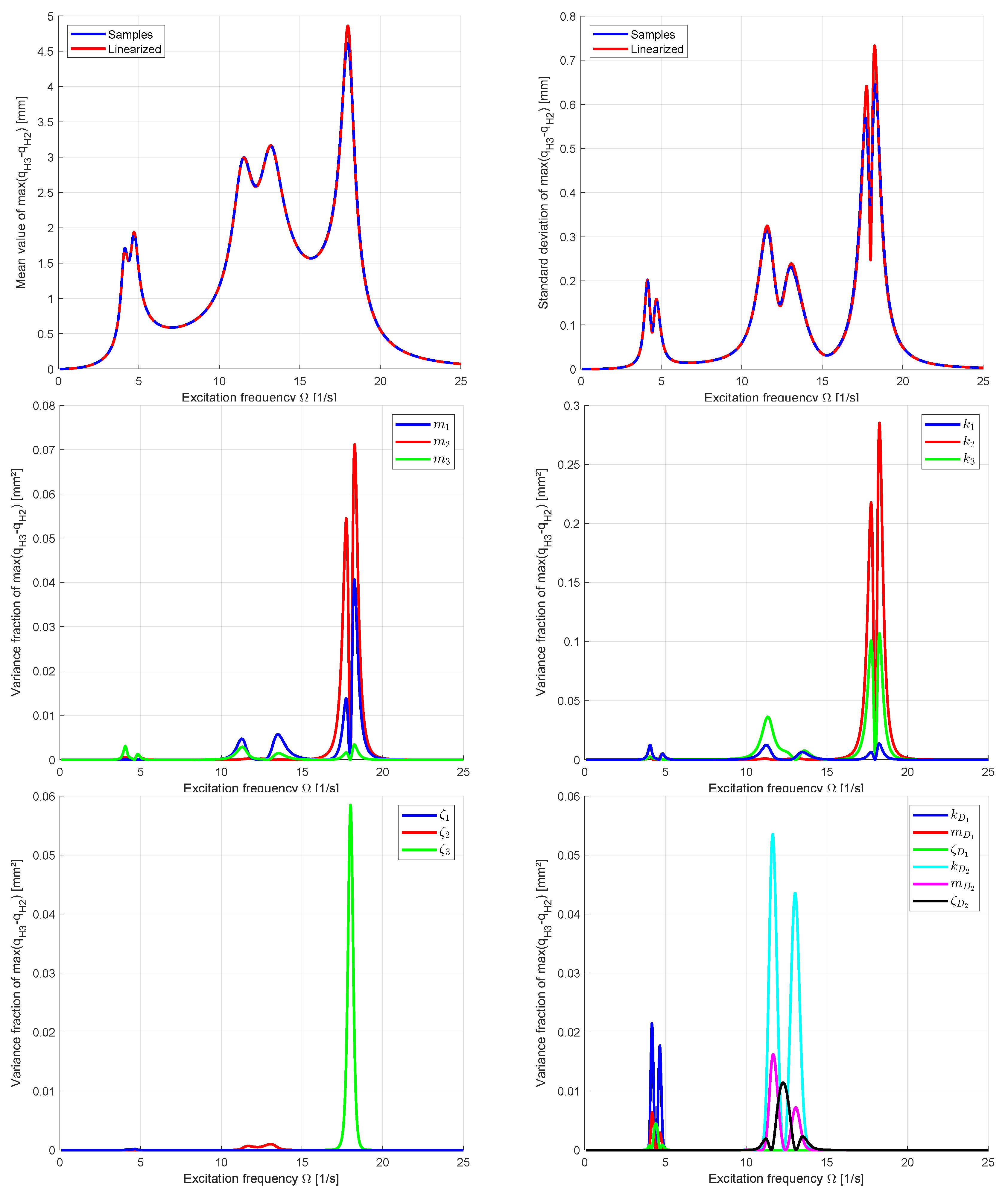
In the next step the uncertainty propagation was investigated for the MDOF example by using 1000 Latin-Hypercube samples and the linearization approach according to Equation (52). The mean values and the scatter of the input parameters were taken according to Table 3. As model responses the maximum displacements of the three original DOFs and the maximum drift between the second and third DOF were evaluated. In Figure 20 the estimated mean values and standard deviations are compared for both approaches depending on the excitation frequency. The figure indicates a very good agreement in the range of the first two natural frequencies, where the TMDs are active. Larger deviations could be observed in the range of the third natural frequency. The variance contribution of the inputs indicate a significant influence of the stiffness and mass coefficients of the main system as well of the modal damping on this displacement variation. However, the scatter of the TMD coefficients is significant only for the variation of the drift displacement for an excitation frequency around the first and second natural frequency.
Figure 20.
Mean values (left) and standard deviations (right) of the three main DOFs estimated from 1000 LHS samples and by using the linearization approach
Figure 20.
Mean values (left) and standard deviations (right) of the three main DOFs estimated from 1000 LHS samples and by using the linearization approach
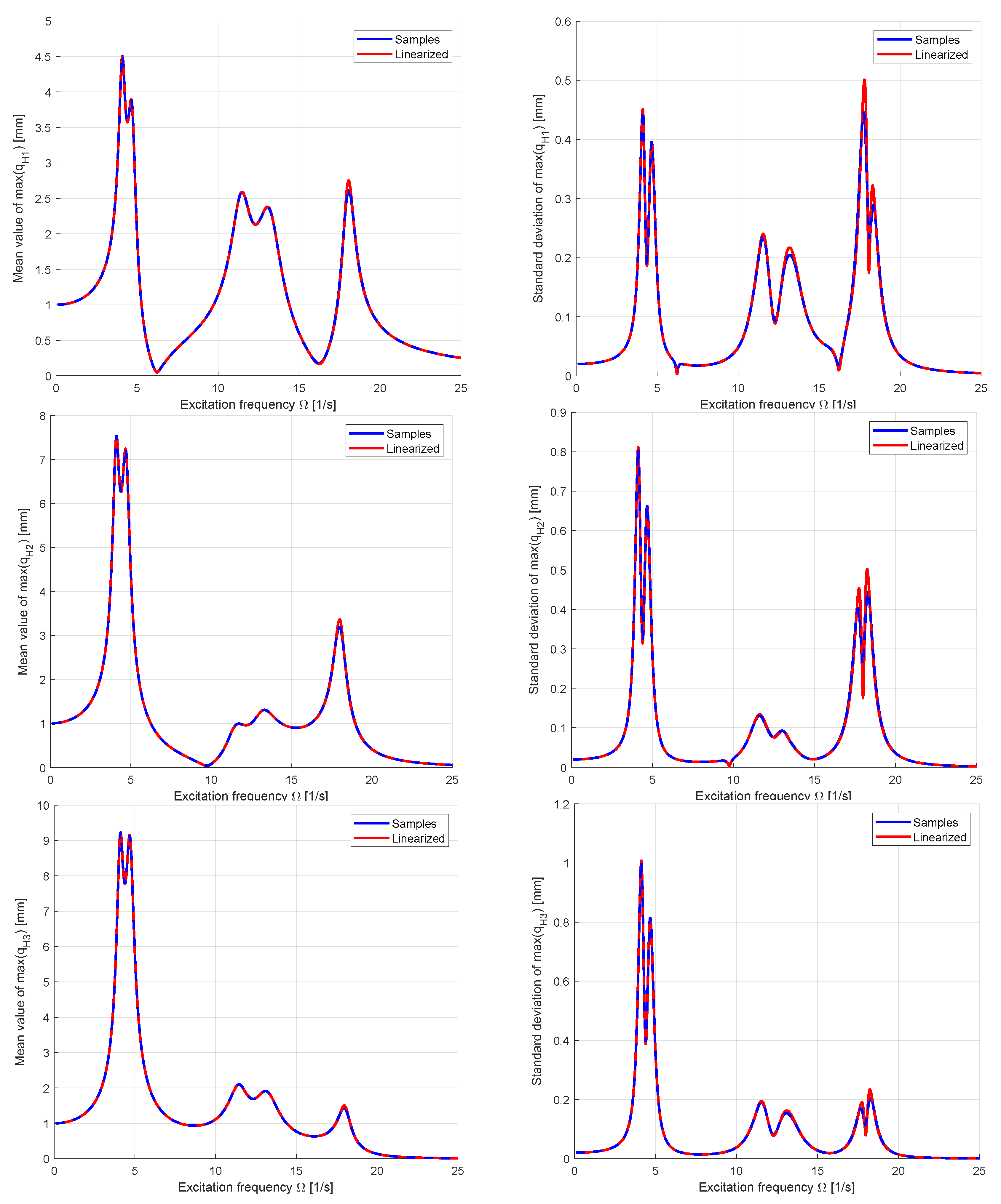
Figure 21.
Mean values and standard deviations of the maximum drift estimated from 1000 LHS samples and by using the linearization approach with the corresponding variance contribution of the input parameters
Figure 21.
Mean values and standard deviations of the maximum drift estimated from 1000 LHS samples and by using the linearization approach with the corresponding variance contribution of the input parameters
3.2.3. Optimization Under Uncertainty
In the final analysis a Robust Design Optimization was performed with different displacement measures: first, the maximum displacement at the third main DOF was considered as one objective and the total mass of both TMDs as another
The evaluated frequency range for the maximum displacement was reduced to to consider only the first two resonance frequencies in the tuning of the TMD parameters.The maximum displacements for the third resonance frequency remain almost constant if the TMD parameters are modified within the optimization. In Figure 22 the maximum mean values and standard deviations of the displacements are shown dependent on the total mass of the TMDs for the deterministic optimization with and for the optimization under uncertainty assuming . As in the SDOF example, a significant reduction of the scatter can be observed for the RDO case while the mean values are slightly increased. The TMD tuned for the second vibration mode gets more mass in the RDO case since the scatter of the displacements around the second resonance is larger as for the first resonance frequency as shown in Figure 23 .
Second, we considered the maximum drift in the upper floor as displacement objective
In Figure 24 the obtained mass distribution of the TMDs is shown with the mean values and standard deviations depending on the excitation frequency. The figure indicates, that the TMD for the second vibration mode obtained much more mass as in the first investigated case. The mean values and the scatter of the maximum displacements are significantly reduced for the considered frequency range while the values around the third resonance remain almost constant. For the robust optimum obtained with the scatter of the maximum drift displacements are significantly reduced compared to the solutions of the deterministic optimization.
4. Conclusions
In this paper we presented an optimization framework for the optimal design of TMDs considering uncertain parameters. We considered the mean and scatter of the amplification function in the optimization goal function of an SDOF system. Since we included the safety margin itself in a variance-based approach, no definition of the limit state function is necessary to obtain an optimal design. The uncertainty propagation was simplified by a linearization approach, which is very efficient compared to a sampling based method. Additionally, the estimated variance of the individual amplification function values is independent of the input distributions and variance-based sensitivity indices can be obtained without additional computational effort. Within the optimization, several goal functions as well as constraints could be considered. We have shown by means of an SDOF example, that the maximum amplification function value is most suitable to obtain minimum displacements. Multi-objective optimization was applied to minimize the maximum displacements and the TMD mass simultaneously. An extension of the presented approach to further constraints e.g. limiting the maximum relative displacements of the TMD is possible in a straight forward manner. Additionally, the amplification function for the accelerations could be considered.
The extension of the presented approach for MDOF systems was introduced as second main contribution of the paper. Instead of using numerically demanding time integration methods, we presented an approximate solution by a decoupled stationary modal approach. Of course, the presented approach is an approximation, nevertheless we could show, that it reaches sufficient accuracy for the optimal design of the TMD parameters. The variance in the investigated response values such as total and relative displacements of the physical DOFs could be approximated with sufficient accuracy with the linearization approach and the robust design optimization could be performed similarly as for the SDOF system. Again, an extension for different response values such as accelerations and relative displacements of the TMDs in the optimization goal functions is straight forward.
So far, we could show, that the procedure itself works for rather simple systems. In further studies, we will apply the presented approach for high rise buildings and pedestrian bridges equipped with tuned mass dampers.
Author Contributions
Conceptualization, T.M., V.Z. and R.R.D.; methodology, T.M., V.Z. and R.R.D.; software, T.M. and A.K.; validation, T.M.; formal analysis, T.M. and A.K.; investigation, T.M. and A.K.; resources, T.M. and V.Z.; data curation, T.M.; writing—original draft preparation, T.M.; writing—review and editing, V.Z. and R.R.D.; visualization, T.M.; supervision, V.Z.; project administration, T.M.; funding acquisition, no funding All authors have read and agreed to the published version of the manuscript.
Funding
This research received no external funding
Institutional Review Board Statement
Not applicable
Informed Consent Statement
Not applicable
Data Availability Statement
The raw data supporting the conclusions of this article will be made available by the authors on request.
Acknowledgments
We acknowledge support for the publication costs by the Open Access Publication Fund of Bauhaus Universität Weimar and the Deutsche Forschungsgemeinschaft (DFG).
Conflicts of Interest
The authors declare no conflicts of interest.
Abbreviations
The following abbreviations are used in this manuscript:
| CoI | Coefficient of Importance |
| CoP | Coefficient of Prognosis |
| CoV | Coefficient of Variation |
| DOF | Degree Of Freedom |
| LHS | Latin Hypercube Sampling |
| MDOF | Multi-Degree-Of-Freedom |
| MOP | Metamodel of Optimal Prognosis |
| NSGA II | Non-dominated Sort Genetic Algorithm |
| RDO | Robust Design Optimization |
| SDOF | Single-Degree-Of-Freedom |
| TMD | Tune Mass Damper |
References
- Ormondroyd, J.; Den Hartog, J. The theory of the dynamic vibration absorber. Journal of Fluids Engineering 1928, 49. [Google Scholar] [CrossRef]
- Gutierrez Soto, M.; Adeli, H. Tuned mass dampers. Archives of Computational Methods in Engineering 2013, 20, 419–431. [Google Scholar] [CrossRef]
- Xu, Y.; Kwok, K.; Samali, B. Control of wind-induced tall building vibration by tuned mass dampers. Journal of Wind Engineering and Industrial Aerodynamics 1992, 40, 1–32. [Google Scholar] [CrossRef]
- Kwok, K.; Samali, B. Performance of tuned mass dampers under wind loads. Engineering structures 1995, 17, 655–667. [Google Scholar] [CrossRef]
- Clark, A.; et al. Multiple passive tuned mass dampers for reducing earthquake induced building motion. In Proceedings of the Proceedings of the 9th world conference on earthquake engineering. Tokyo-Kyoto JAPAN, 1988, Vol. 5, pp. 779–784.
- Sadek, F.; Mohraz, B.; Taylor, A.; Chung, R. A method of estimating the parameters of tuned mass dampers for seismic applications. Earthquake Engineering & Structural Dynamics 1997, 26, 617–635. [Google Scholar] [CrossRef]
- Warburton, G.B. Optimum absorber parameters for various combinations of response and excitation parameters. Earthquake Engineering & Structural Dynamics 1982, 10, 381–401. [Google Scholar] [CrossRef]
- Wang, Y.; Cheng, S. The optimal design of dynamic absorber in the time domain and the frequency domain. Applied Acoustics 1989, 28, 67–78. [Google Scholar] [CrossRef]
- Petersen, C.; Werkle, H. Dynamik der Baukonstruktionen, 2 ed.; Springer Viehweg: Wiesbaden, Germany, 2017. [Google Scholar]
- Rana, R.; Soong, T. Parametric study and simplified design of tuned mass dampers. Engineering structures 1998, 20, 193–204. [Google Scholar] [CrossRef]
- Lee, C.L.; Chen, Y.T.; Chung, L.L.; Wang, Y.P. Optimal design theories and applications of tuned mass dampers. Engineering structures 2006, 28, 43–53. [Google Scholar] [CrossRef]
- Colherinhas, G.; de Morais, M.; Shzu, M.; Avila, S. Optimal pendulum tuned mass damper design applied to high towers using genetic algorithms: Two-DOF modeling. International Journal of Structural Stability and Dynamics 2019, 19, 1950125. [Google Scholar] [CrossRef]
- Hadi, M.; Arfiadi, Y. Optimum design of absorber for MDOF structures. Journal of Structural Engineering 1998, 124, 1272–1280. [Google Scholar] [CrossRef]
- Hoang, N.; Warnitchai, P. Design of multiple tuned mass dampers by using a numerical optimizer. Earthquake engineering & structural dynamics 2005, 34, 125–144. [Google Scholar] [CrossRef]
- Zuo, L.; Nayfeh, S. Optimization of the individual stiffness and damping parameters in multiple-tuned-mass-damper systems. Journal of Vibration and Acoustics 2005, 127, 77–83. [Google Scholar] [CrossRef]
- Elias, S.; Matsagar, V. Research developments in vibration control of structures using passive tuned mass dampers. Annual Reviews in Control 2017, 44, 129–156. [Google Scholar] [CrossRef]
- Yang, F.; Sedaghati, R.; Esmailzadeh, E. Vibration suppression of structures using tuned mass damper technology: A state-of-the-art review. Journal of Vibration and Control 2022, 28, 812–836. [Google Scholar] [CrossRef]
- Leung, A.; Zhang, H. Particle swarm optimization of tuned mass dampers. Engineering Structures 2009, 31, 715–728. [Google Scholar] [CrossRef]
- Arfiadi, Y. Optimum placement and properties of tuned mass dampers using hybrid genetic algorithms. International Journal of Optimization in Civil Engineering 2011, 1, 167. [Google Scholar]
- R.H., R.; Könke, C. Seismic control of tall buildings using distributed multiple tuned mass dampers. Advances in Civil Engineering 2019, 2019, 6480384. [Google Scholar] [CrossRef]
- Yucel, M.; Bekdaş, G.; Nigdeli, S.; Sevgen, S. Estimation of optimum tuned mass damper parameters via machine learning. Journal of Building Engineering 2019, 26, 100847. [Google Scholar] [CrossRef]
- Yucel, M.; Bekdaş, G.; Nigdeli, S. Machine learning-based model for prediction of optimum TMD parameters in time-domain history. Journal of the Brazilian Society of Mechanical Sciences and Engineering 2024, 46, 192. [Google Scholar] [CrossRef]
- Papadimitriou, C.; Katafygiotis, L.; Au, S.K. Effects of structural uncertainties on TMD design: A reliability-based approach. Journal of Structural Control 1997, 4, 65–88. [Google Scholar] [CrossRef]
- Hu, W. Design Optimization Under Uncertainty; Springer, 2023.
- Moreno, C.; Thomson, P. Design of an optimal tuned mass damper for a system with parametric uncertainty. Annals of Operations Research 2010, 181, 783–793. [Google Scholar] [CrossRef]
- Schmelzer, B.; Oberguggenberger, M.; Adam, C. Efficiency of tuned mass dampers with uncertain parameters on the performance of structures under stochastic excitation. Proceedings of the Institution of Mechanical Engineers, Part O: Journal of Risk and Reliability 2010, 224, 297–308. [Google Scholar] [CrossRef]
- Khalid, M.; Bansal, S. Framework for Robust Design Optimization of Tuned Mass Dampers by Stochastic Subset Optimization. International Journal of Structural Stability and Dynamics 2023, 23, 2350155. [Google Scholar] [CrossRef]
- Song, C.; Xiao, R.; Jiang, Z.; Sun, B. Active-learning Kriging-assisted robust design optimization of tuned mass dampers: Vibration mitigation of a steel-arch footbridge. Engineering Structures 2024, 303, 117502. [Google Scholar] [CrossRef]
- Pellizzari, F.; Marano, G.; Palmeri, A.; Greco, R.; Domaneschi, M. Robust optimization of MTMD systems for the control of vibrations. Probabilistic Engineering Mechanics 2022, 70, 103347. [Google Scholar] [CrossRef]
- Shamsaddinlou, A.; Shirgir, S.; Hadidi, A.; Azar, B. An efficient reliability-based design of TMD & MTMD in nonlinear structures under uncertainty. In Proceedings of the Structures. Elsevier, 2023, Vol. 51, pp. 258–274.
- Li, D.; Tang, H.; Xue, S. Robust design of tuned mass damper with hybrid uncertainty. Structural Control and Health Monitoring 2021, 28, e2803. [Google Scholar] [CrossRef]
- Sreeman, D.; Roy, B. Robust design optimization of the friction pendulum system isolated building considering system parameter uncertainties under seismic excitations. Journal of Building Engineering 2024, 82, 108320. [Google Scholar] [CrossRef]
- Seesselberg, C. Basiswissen Baudynamik - Grundlagen und Anwendungen; Beuth Verlag GmbH: Berlin, Wien, Zürich, 2022. [Google Scholar]
- Eibl, J.; Häussler-Combe, U. Baudynamik. In Betonkalender 1997; 1997; pp. 755–863.
- Chopra, A. Dynamics of Structures, 5 ed.; Pearson Education, Inc.: Uttar Pradesh, India, 2017.
- Haftka, R.; Gürdal, Z. Elements of structural optimization; Kluwer Academic Publishers: Dordrecht, The Netherlands, 1992.
- Luersen, M.A.; Le Riche, R.; Guyon, F. A constrained, globalized, and bounded Nelder–Mead method for engineering optimization. Structural and Multidisciplinary Optimization 2004, 27, 43–54. [Google Scholar] [CrossRef]
- Deb, K.; Pratap, A.; Agarwal, S.; Meyarivan, T. A fast and elitist multiobjective genetic algorithm: NSGA-II. IEEE transactions on evolutionary computation 2002, 6, 182–197. [Google Scholar] [CrossRef]
- Rubinstein, R.Y. Simulation and the Monte Carlo Method; John Wiley & Sons: New York, 1981.
- Nataf, A. Détermination des distributions de probabilités dont les marges sont données. Comptes Rendus de l’Academie des Sciences 1962, 225, 42–43. [Google Scholar]
- Bucher, C. Computational analysis of randomness in structural mechanics; CRC Press, Taylor & Francis Group: London, 2009.
- Huntington, D.; Lyrintzis, C. Improvements to and limitations of Latin hypercube sampling. Probabilistic engineering mechanics 1998, 13, 245–253. [Google Scholar] [CrossRef]
- Sobol’, I.M. Sensitivity estimates for nonlinear mathematical models. Mathematical Modelling and Computational Experiment 1993, 1, 407–414. [Google Scholar]
- Homma, T.; Saltelli, A. Importance measures in global sensitivity analysis of nonlinear models. Reliability Engineering and System Safety 1996, 52, 1–17. [Google Scholar] [CrossRef]
- Saltelli, A.; et al. Global Sensitivity Analysis. The Primer; John Wiley & Sons, Ltd: Chichester, England, 2008.
- Most, T.; Will, J. Sensitivity analysis using the Metamodel of Optimal Prognosis. In Proceedings of the 8th Optimization and Stochastic Days, Weimar, Germany, 24-25 November, 2011, 2011. [CrossRef]
- Myers, R.H.; Montgomery, D.C. Response surface methodology: process and product optimization using designed experiments; John Wiley & Sons, 2002.
- Krige, D. A statistical approach to some basic mine valuation problems on the Witwatersrand. Journal of the Chemical, Metallurgical and Mining Society of South Africa 1951, 52, 119–139. [Google Scholar]
- Lancaster, P.; Salkauskas, K. Surface generated by moving least squares methods. Mathematics of Computation 1981, 37, 141–158. [Google Scholar] [CrossRef]
- Hagan, M.T.; Demuth, H.B.; Beale, M. Neural Network Design; PWS Publishing Company, 1996.
- Ansys Germany GmbH. Ansys optiSLang user documentation. Weimar, Germany, 2025R1 ed., 2025. https://www.ansys.com/de-de/products/connect/ansys-optislang Accessed: 2025-06-18.
- Most, T.; Gräning, L.; Wolff, S. Robustness investigation of cross-validation based quality measures for model assessment. Engineering Modelling, Analysis and Simulation 2024, 2. [Google Scholar] [CrossRef]
- Most, T. Variance-based sensitivity analysis in the presence of correlated input variables. In 5th International Conference on Reliable Engineering Computing (REC), Brno, Czech Republic, 13-15 June, 2012; 2012; pp. 335–352.
- Koch, P.; Yang, R.J.; Gu, L. Design for six sigma through robust optimization. Structural and Multidisciplinary Optimization 2004, 26, 235–248. [Google Scholar] [CrossRef]
- Most, T.; Will, J. Robust Design Optimization in industrial virtual product development. In 5th International Conference on Reliable Engineering Computing (REC), Brno, Czech Republic, 13-15 June, 2012; 2012; pp. 353–366.
- The European Union. EN 1990 (2002) (English): Eurocode - Basis of structural design, Regulation 305/2011. 2002.
- Khadka, A. Optimization of tuned mass dampers in multi-degree-of-freedom systems. Master thesis, Bauhaus-Universität Weimar, 2025.
Figure 1.
Pedestrian bridge with vibration damper, transfer to a mechanical beam model with attached damper and abstraction as dynamical 2-degree-of-freedom system (photos [33])
Figure 1.
Pedestrian bridge with vibration damper, transfer to a mechanical beam model with attached damper and abstraction as dynamical 2-degree-of-freedom system (photos [33])
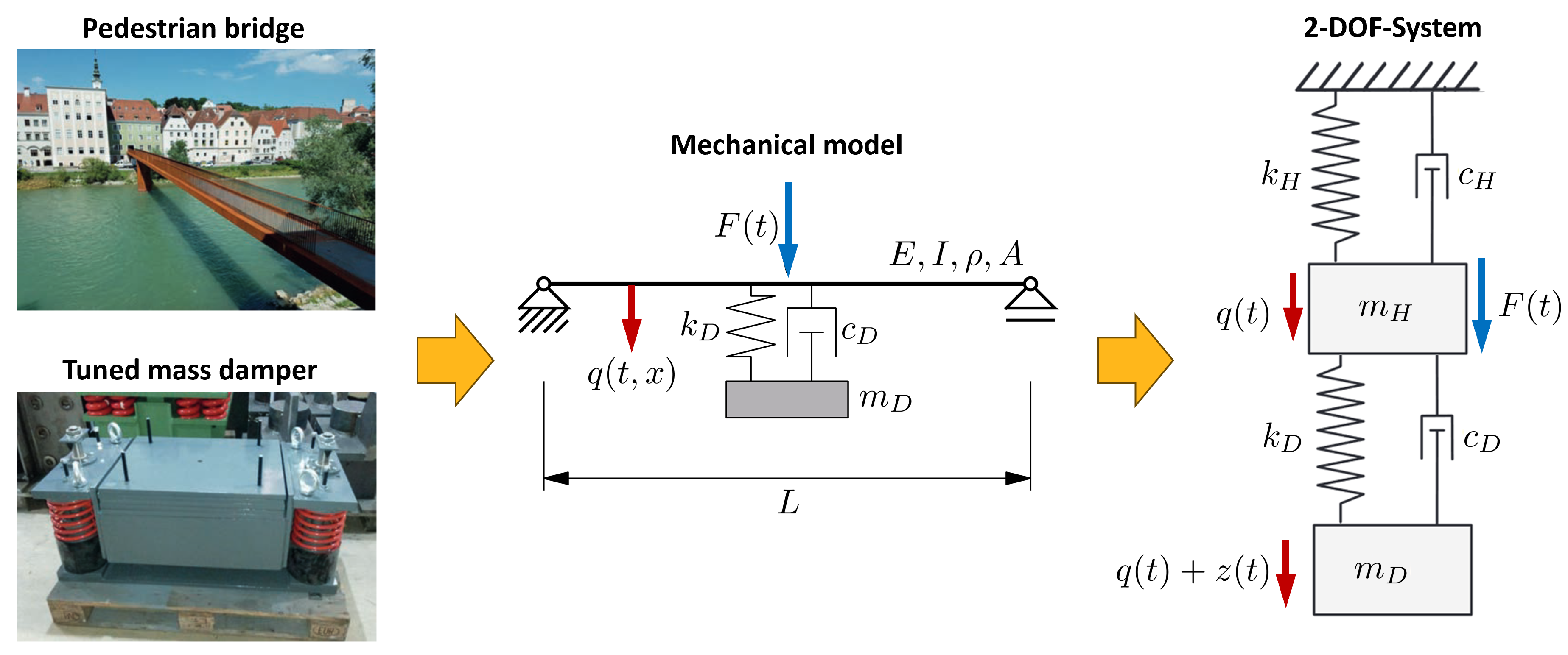
Figure 2.
Dynamic amplification functions of an SDOF-system with a damping ratio without TMD and with optimal TMD parameters according to Den Hartog for different mass ratios
Figure 2.
Dynamic amplification functions of an SDOF-system with a damping ratio without TMD and with optimal TMD parameters according to Den Hartog for different mass ratios
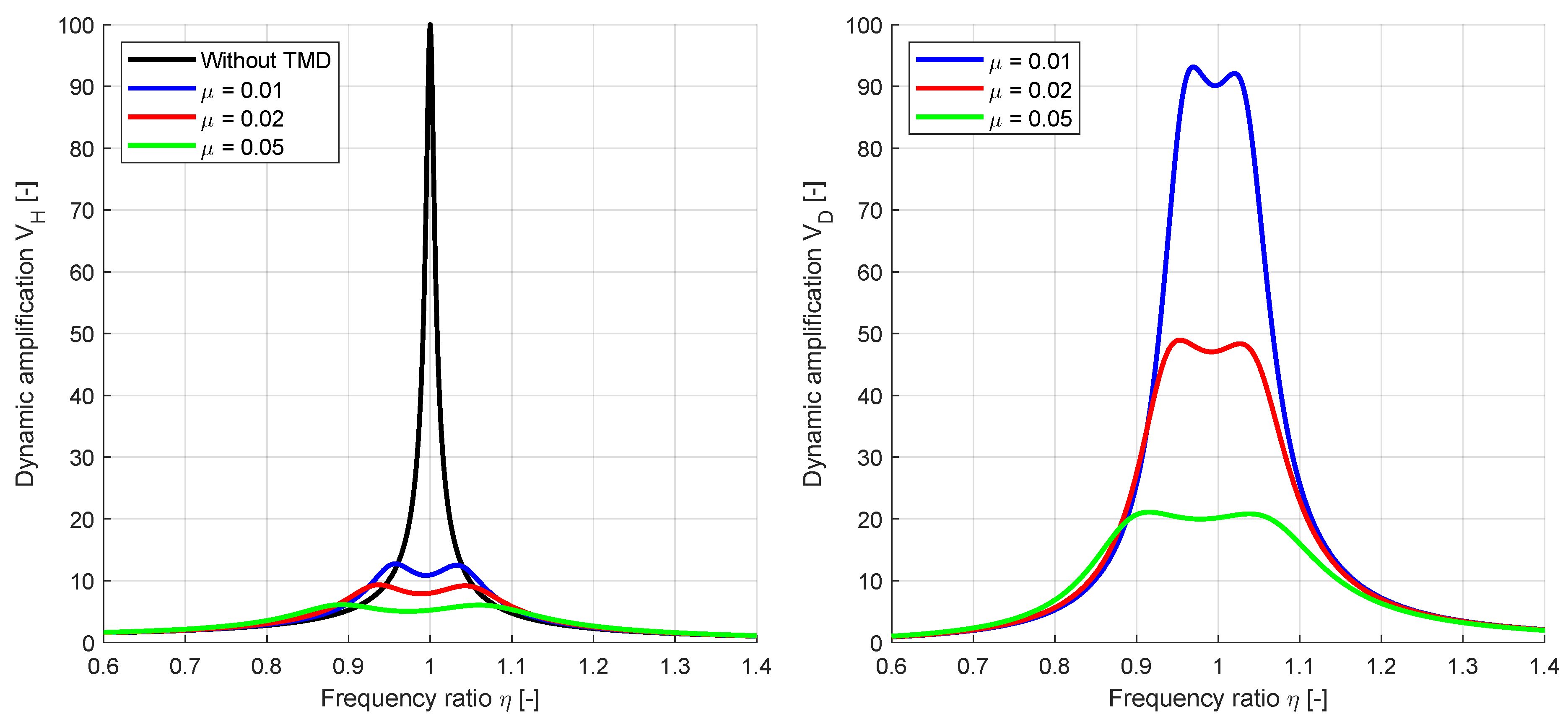
Figure 3.
Pareto optimal designs on the Pareto frontier for two conflicting objectives (left) and the principle of the non-dominated sort approach used in the NSGA-II algorithm (right)
Figure 3.
Pareto optimal designs on the Pareto frontier for two conflicting objectives (left) and the principle of the non-dominated sort approach used in the NSGA-II algorithm (right)
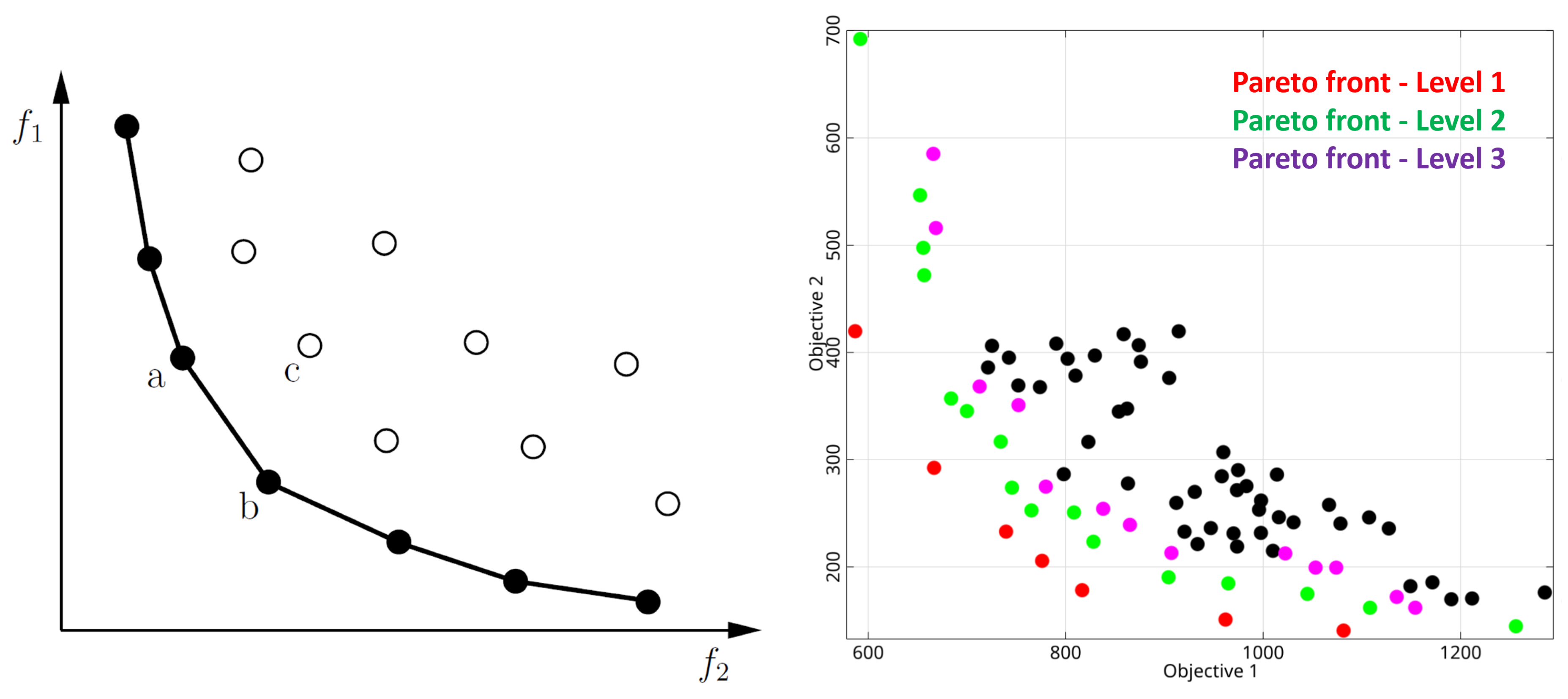
Figure 4.
Representation of marginals of random input parameters with equal probability classes and minimized spurious correlations within the improved Latin Hypercube sampling
Figure 4.
Representation of marginals of random input parameters with equal probability classes and minimized spurious correlations within the improved Latin Hypercube sampling
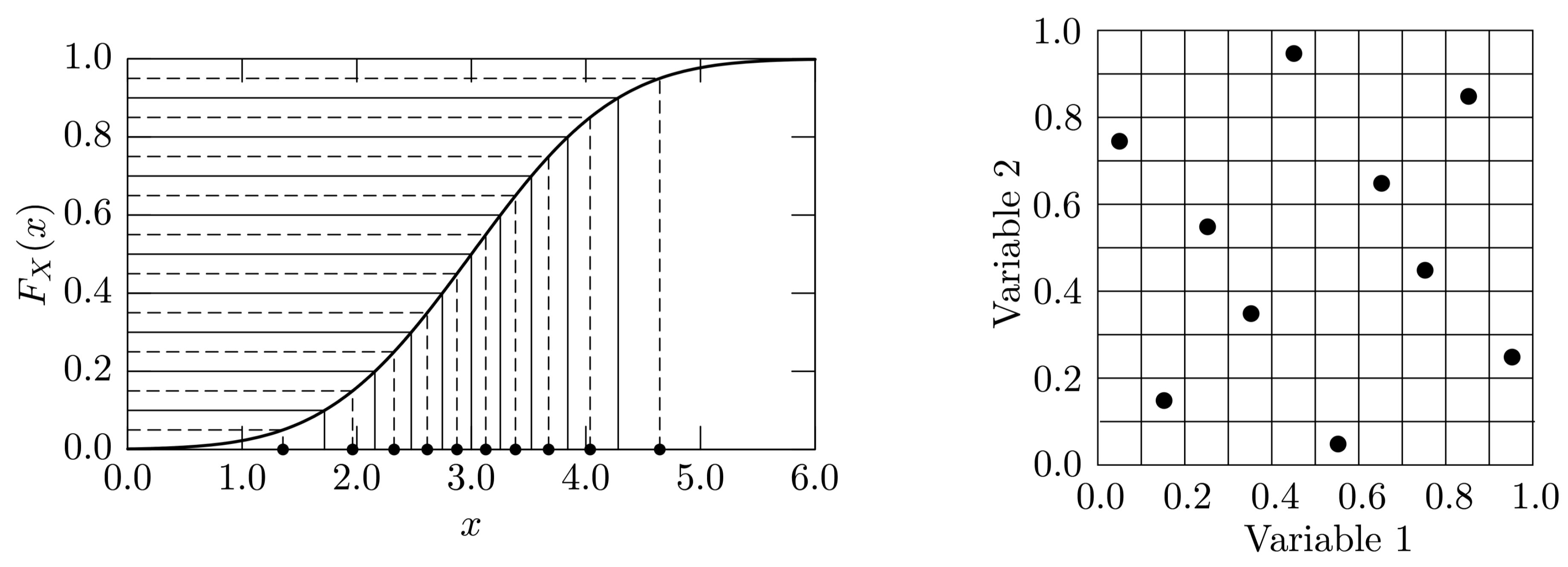
Figure 5.
A random response with indicated limit and corresponding exceedance probability and the safety margin between the mean value and the limit
Figure 5.
A random response with indicated limit and corresponding exceedance probability and the safety margin between the mean value and the limit
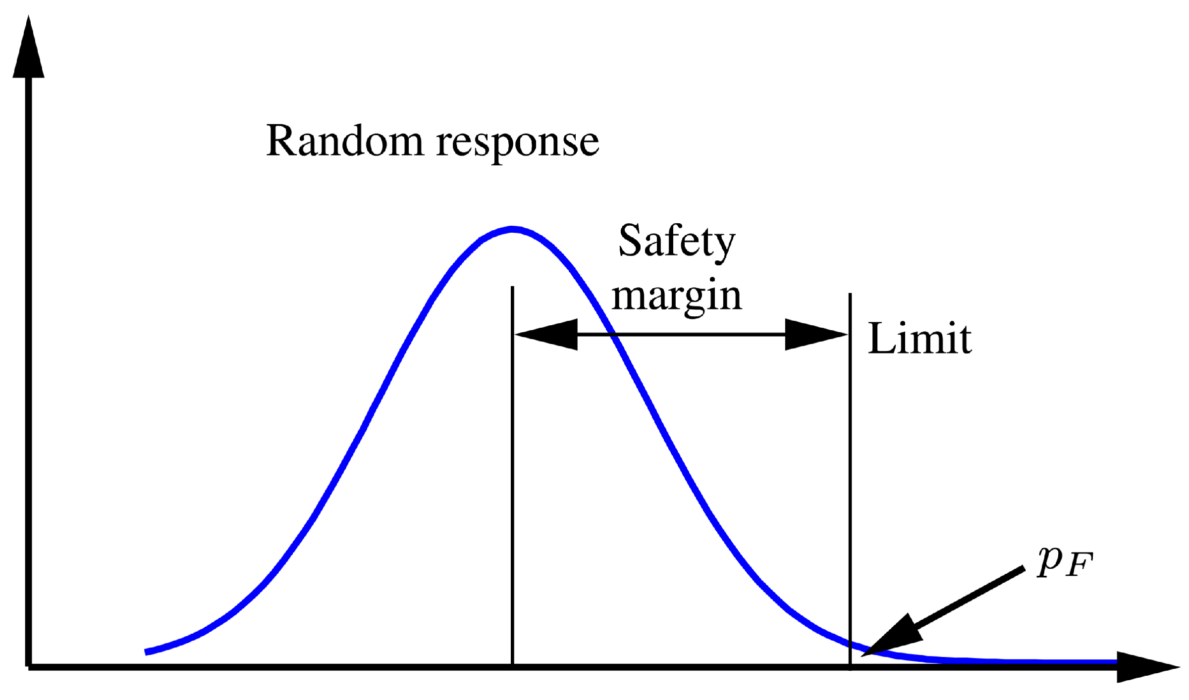
Figure 6.
Superposition of the displacements of an MDOF-system with a single TMD optimized for the first vibration mode
Figure 6.
Superposition of the displacements of an MDOF-system with a single TMD optimized for the first vibration mode
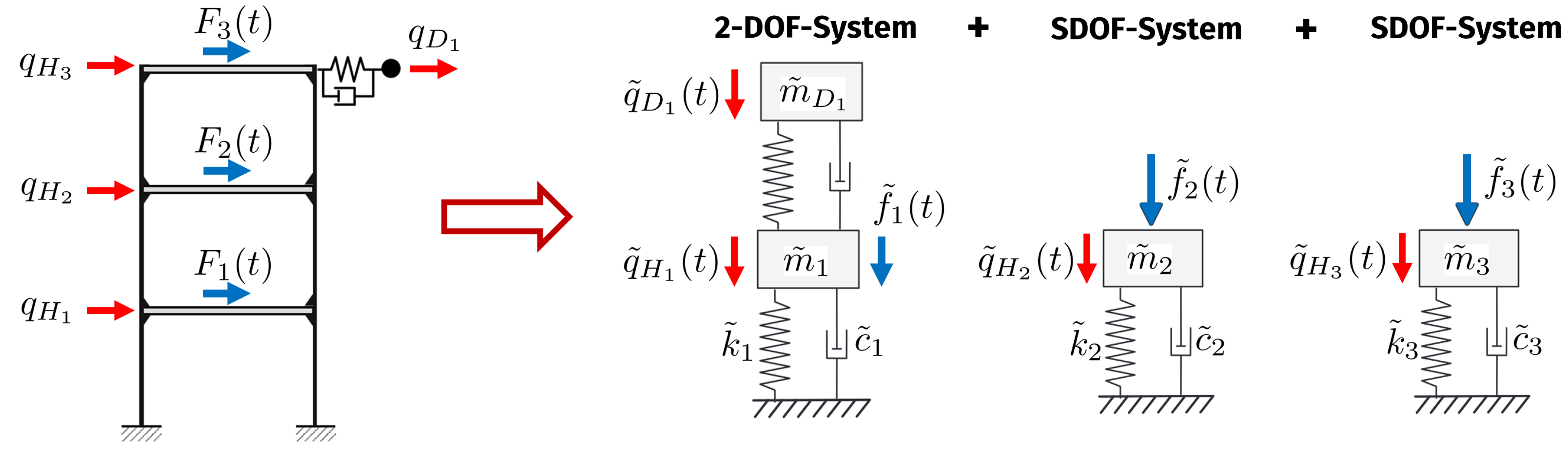
Figure 7.
Objective functions max(VH(η)) (left) and VH(η = 1.0) (right) with the optimum parameters according to Den Hartog (red dot) for a mass ratio of µ = 2.0%
Figure 7.
Objective functions max(VH(η)) (left) and VH(η = 1.0) (right) with the optimum parameters according to Den Hartog (red dot) for a mass ratio of µ = 2.0%
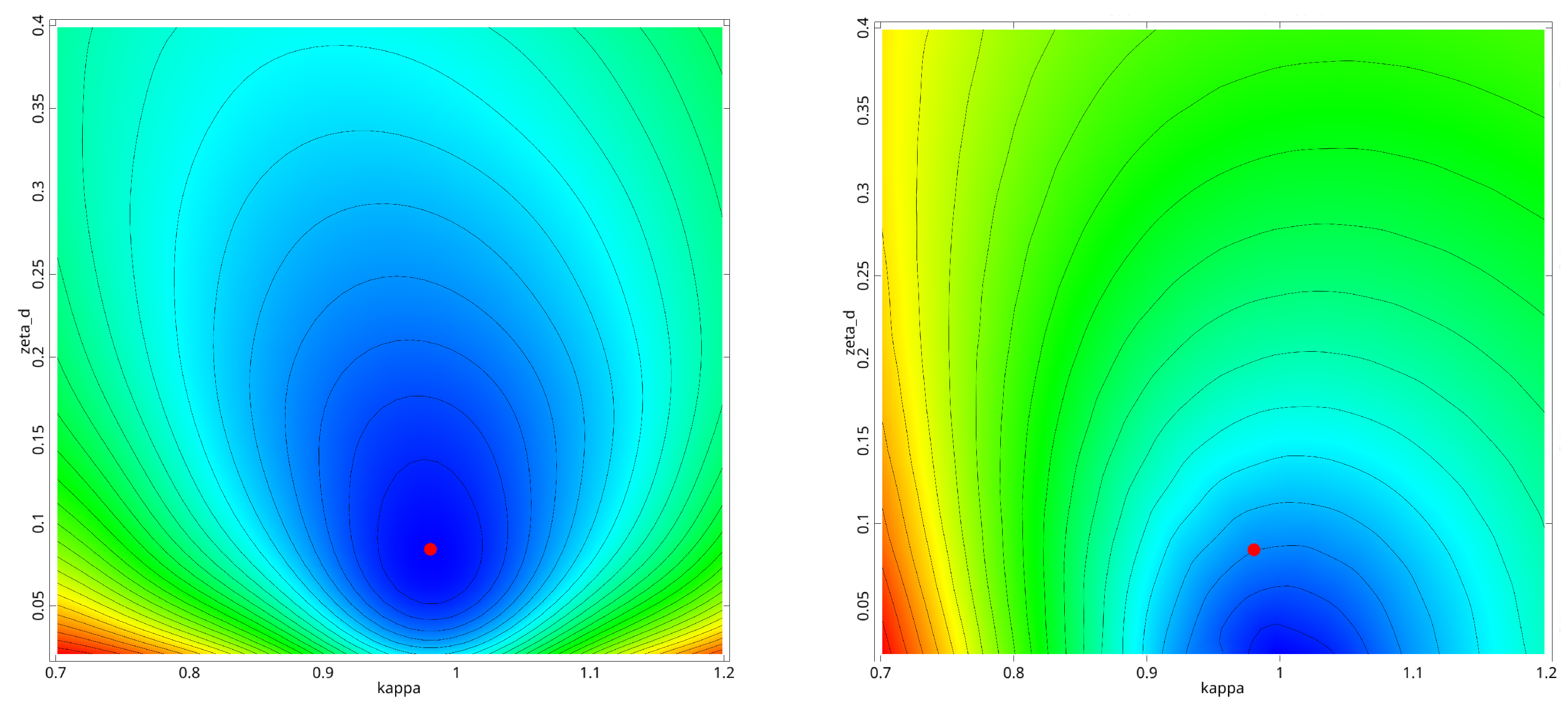
Figure 8.
Amplification functions with optimal parameters according to Den Hartog and from single-objective optimization by minimizing and
Figure 8.
Amplification functions with optimal parameters according to Den Hartog and from single-objective optimization by minimizing and

Figure 9.
Results of the multi-objective optimization, several single-objective optimization runs with different mass ratios and the corresponding optimal parameters according to Den Hartog for the SDOF example
Figure 9.
Results of the multi-objective optimization, several single-objective optimization runs with different mass ratios and the corresponding optimal parameters according to Den Hartog for the SDOF example
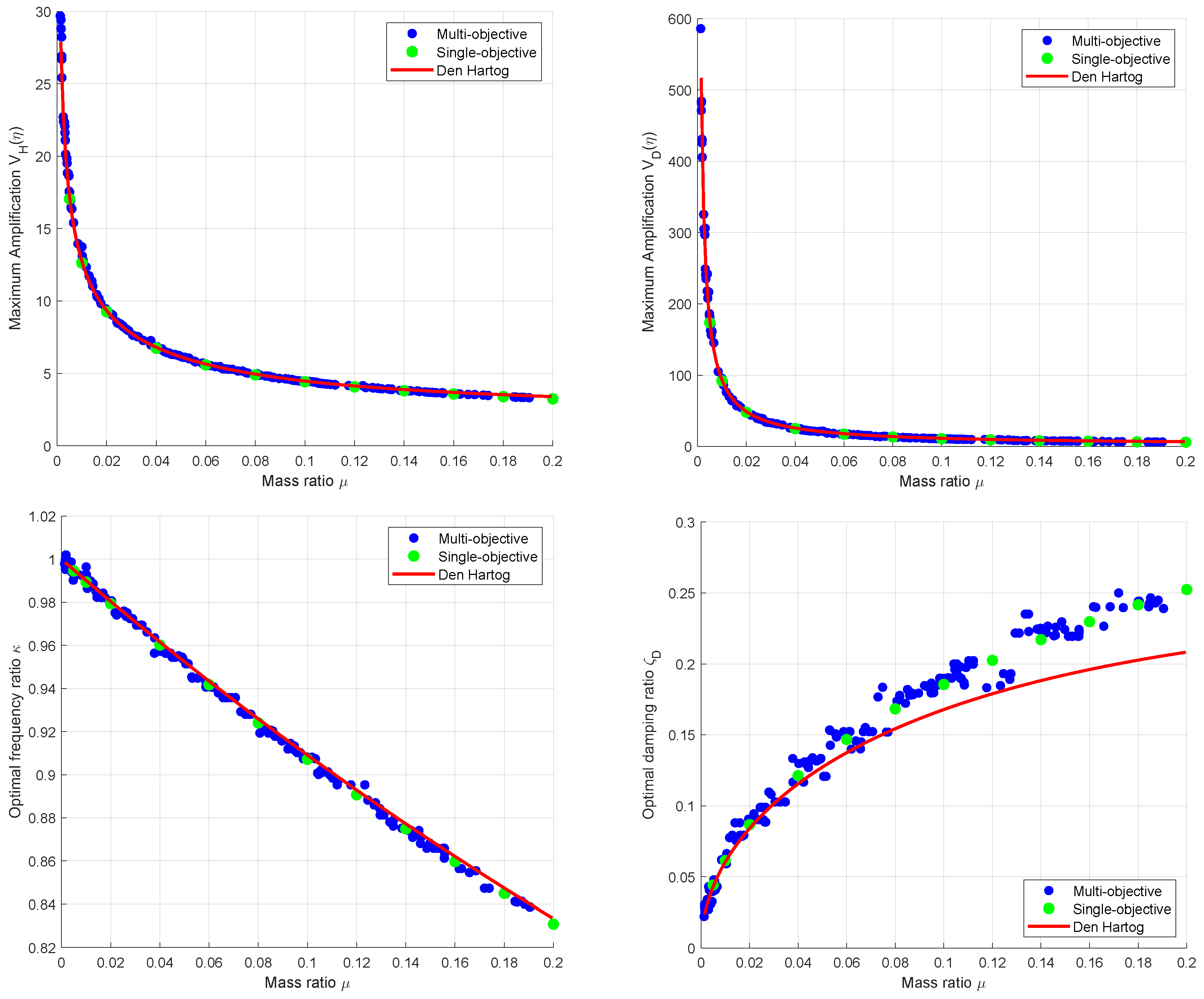
Figure 10.
100 Latin Hypercube samples of the amplification functions of the SDOF example compared to the deterministic functions according to Den Hartog for a nominal mass ratio of
Figure 10.
100 Latin Hypercube samples of the amplification functions of the SDOF example compared to the deterministic functions according to Den Hartog for a nominal mass ratio of
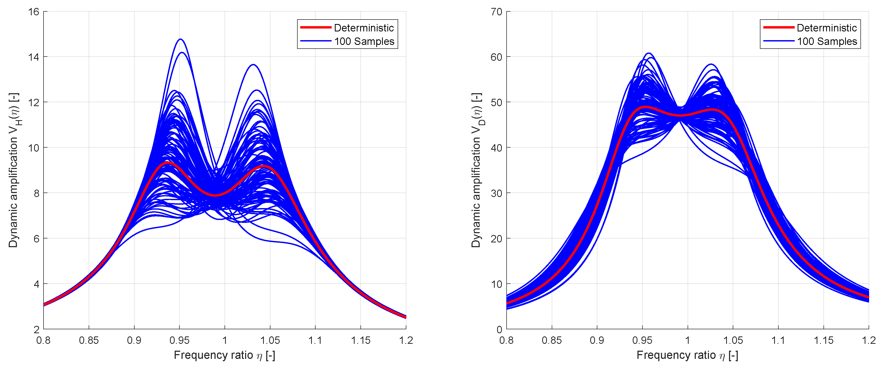
Figure 11.
Approximated response functions of the amplification values , and including the sensitivity indices using linear and quadratic regression models and the MOP approximation for a nominal mass ratio of
Figure 11.
Approximated response functions of the amplification values , and including the sensitivity indices using linear and quadratic regression models and the MOP approximation for a nominal mass ratio of
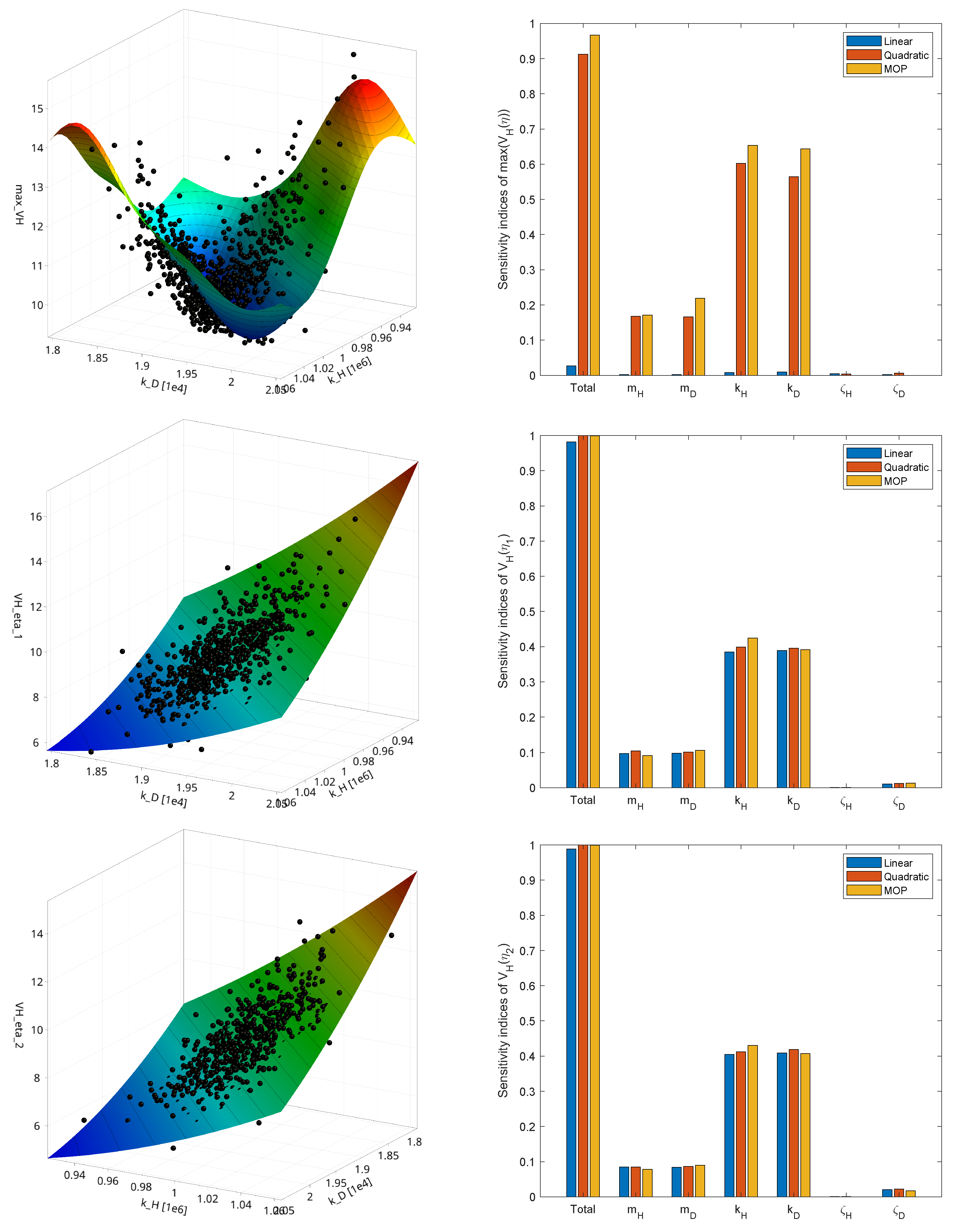
Figure 12.
Mean value (top), standard deviation (middle) of the amplification function values for a nominal mass ratio of estimated from 1000 LHS samples and by using the linearization approach with the corresponding variance contribution of the input parameters (bottom)
Figure 12.
Mean value (top), standard deviation (middle) of the amplification function values for a nominal mass ratio of estimated from 1000 LHS samples and by using the linearization approach with the corresponding variance contribution of the input parameters (bottom)
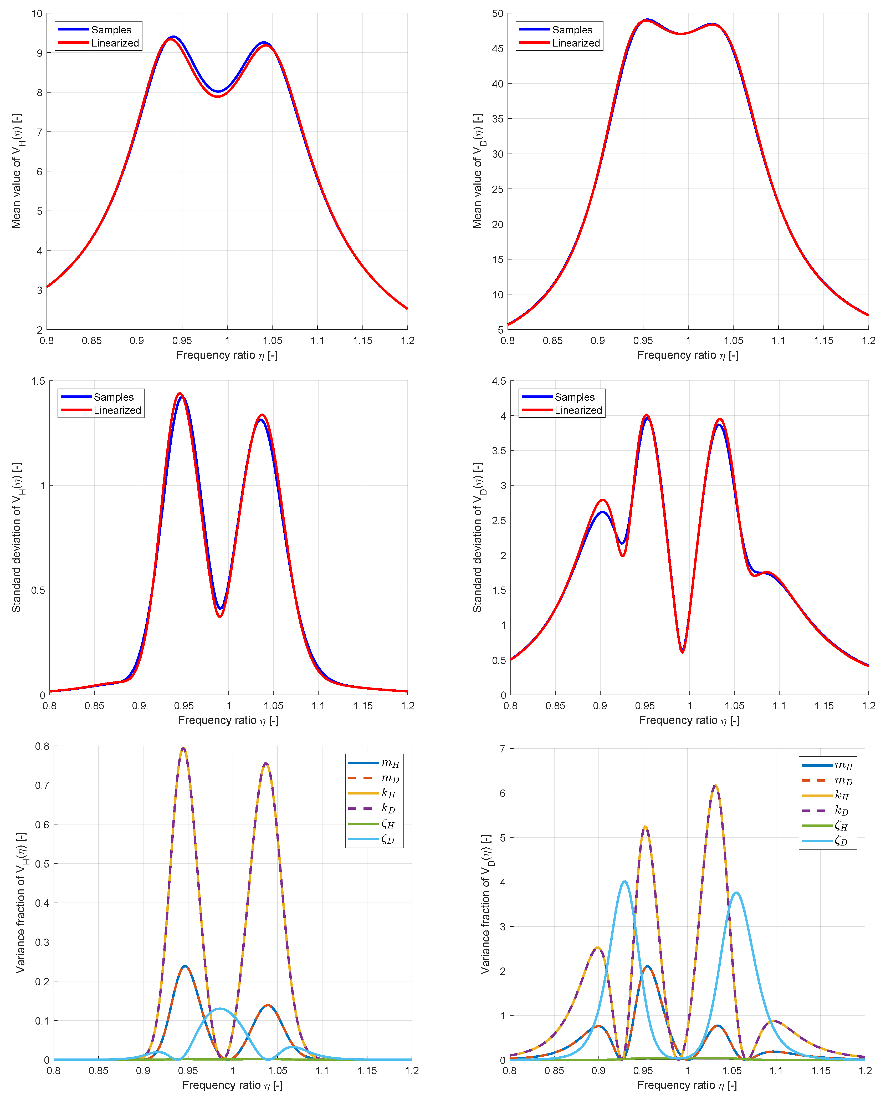
Figure 13.
Maximum mean value (left) and standard deviation (right) of as a function of the optimization parameters and as well as the deterministic optimum (red), the optimum (green) and the optimum (yellow)
Figure 13.
Maximum mean value (left) and standard deviation (right) of as a function of the optimization parameters and as well as the deterministic optimum (red), the optimum (green) and the optimum (yellow)
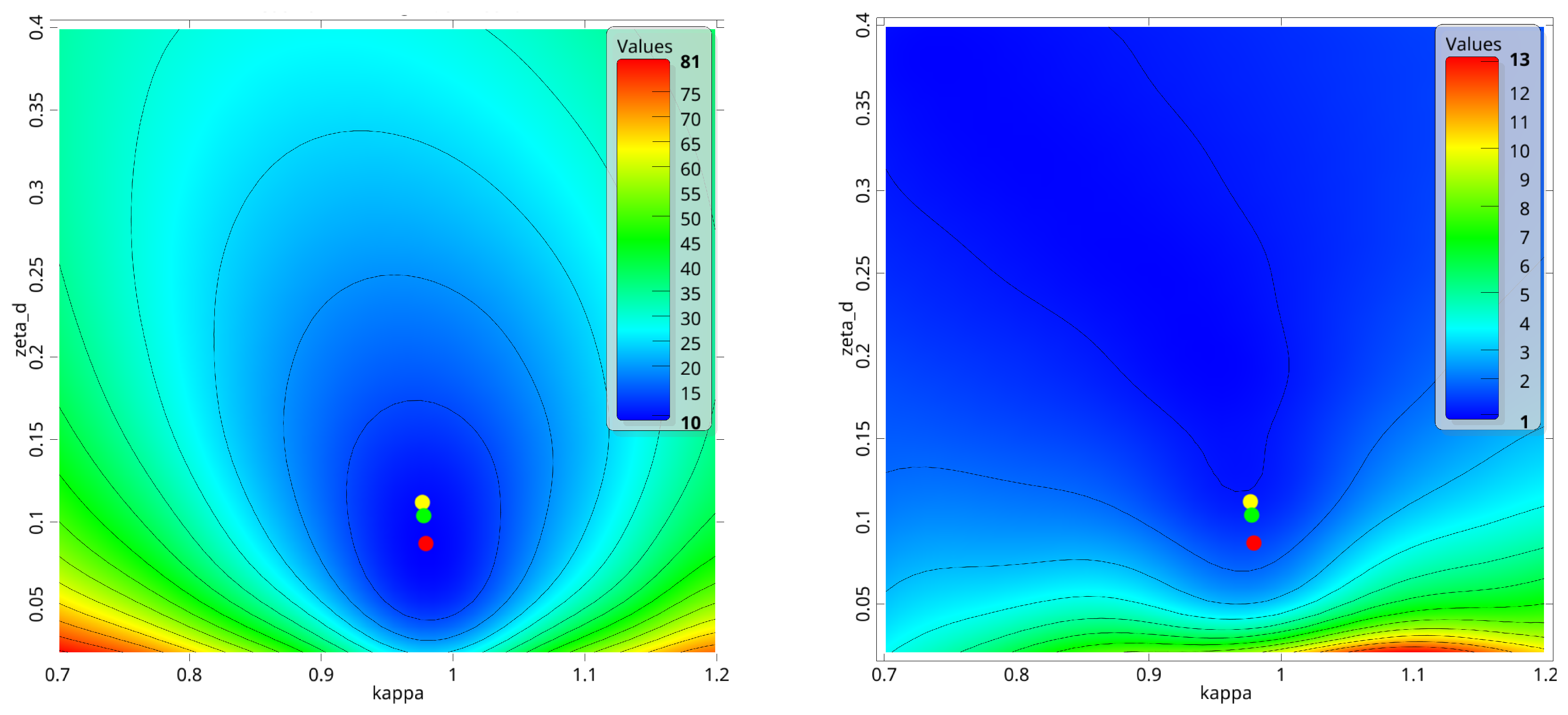
Figure 14.
Estimated mean values and 4.7-fold standard deviations for the function values of and for the deterministic optimum and for a safety margin of
Figure 14.
Estimated mean values and 4.7-fold standard deviations for the function values of and for the deterministic optimum and for a safety margin of
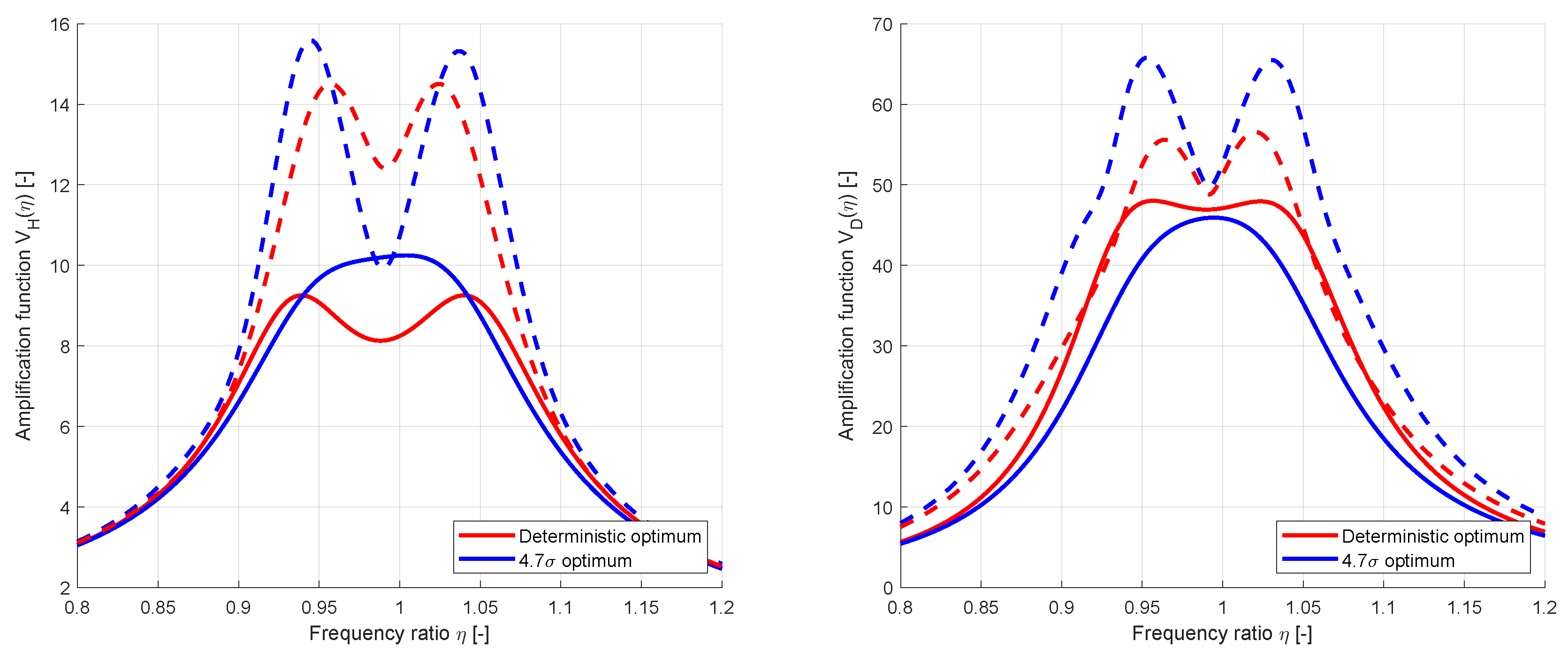
Figure 15.
Optimized maximum mean value and standard deviation of the amplification function values and corresponding nominal values of and for an increasing nominal mass ratio and different safety margins for the SDOF example
Figure 15.
Optimized maximum mean value and standard deviation of the amplification function values and corresponding nominal values of and for an increasing nominal mass ratio and different safety margins for the SDOF example
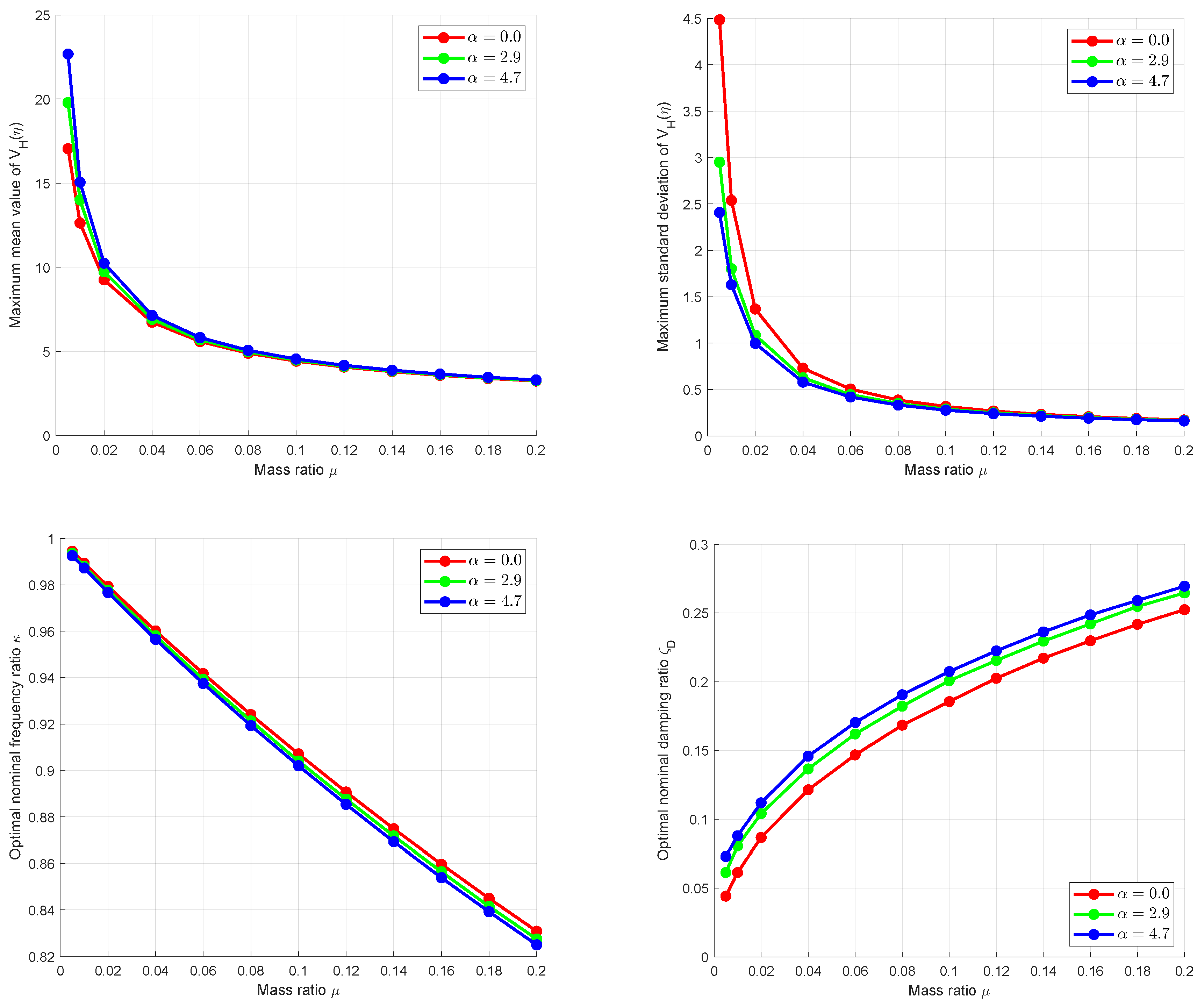
Figure 19.
Approximated stationary displacements of the MDOF example compared with Newmark results for the original DOFs, the second floor drift and the relative displacements of the TMDs
Figure 19.
Approximated stationary displacements of the MDOF example compared with Newmark results for the original DOFs, the second floor drift and the relative displacements of the TMDs
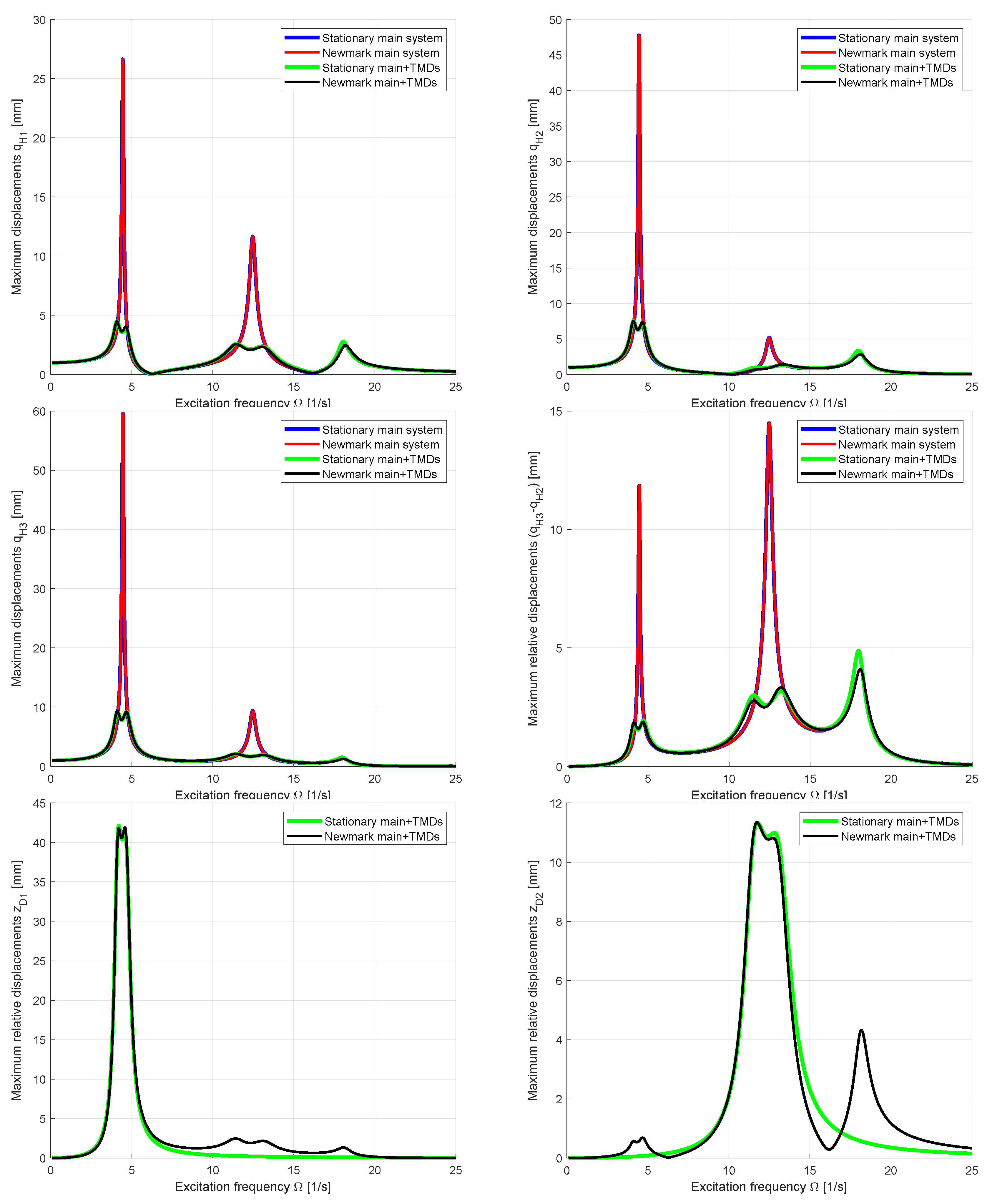
Figure 22.
Optimized maximum mean values and standard deviations of the maximum displacement of for an increasing mass of the TMDs and different safety margins for the MDOF example
Figure 22.
Optimized maximum mean values and standard deviations of the maximum displacement of for an increasing mass of the TMDs and different safety margins for the MDOF example
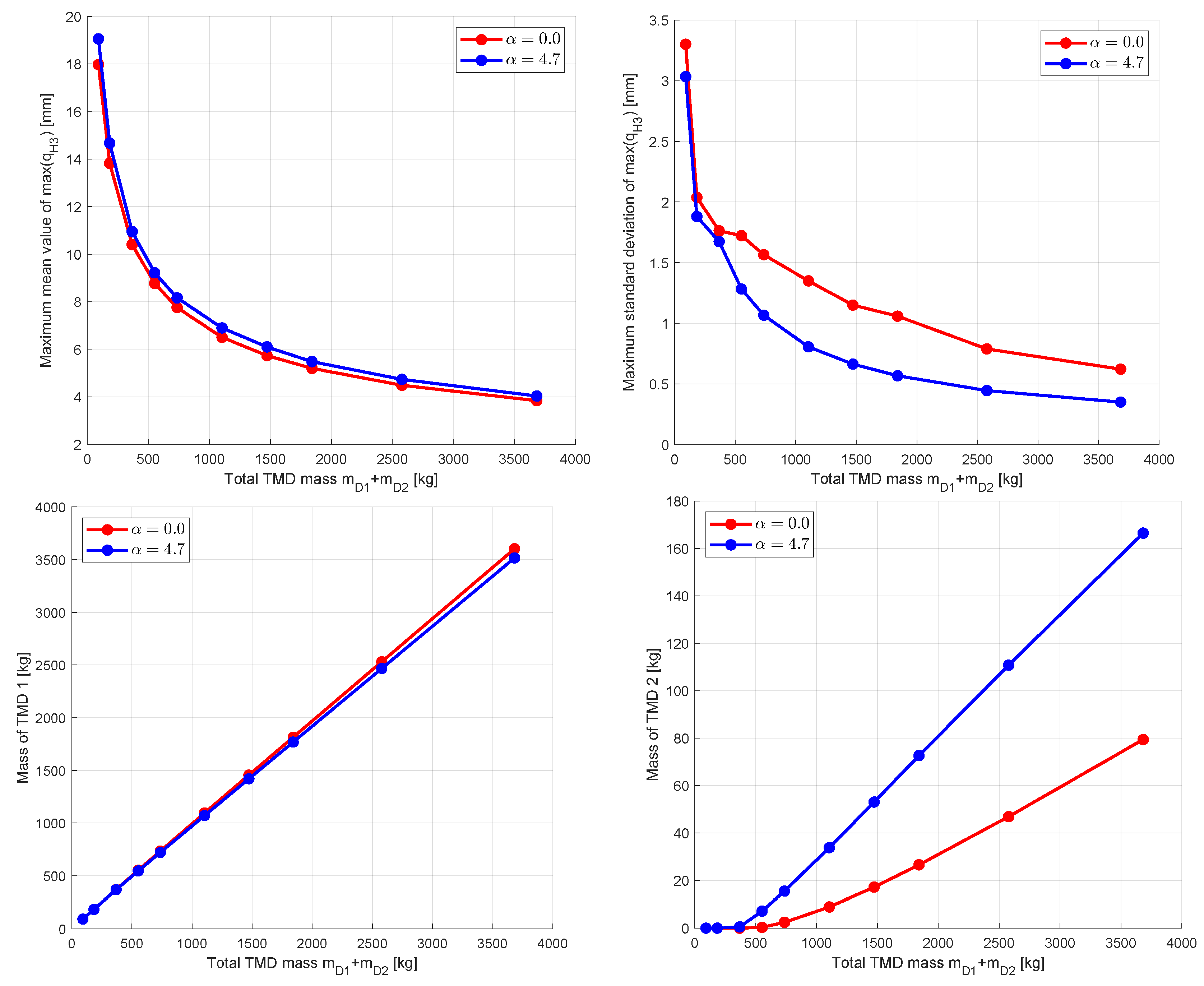
Figure 23.
Mean values and standard deviations of the maximum displacements for an increasing mass of the TMDs dependent on the excitation frequancy and the safety margin
Figure 23.
Mean values and standard deviations of the maximum displacements for an increasing mass of the TMDs dependent on the excitation frequancy and the safety margin
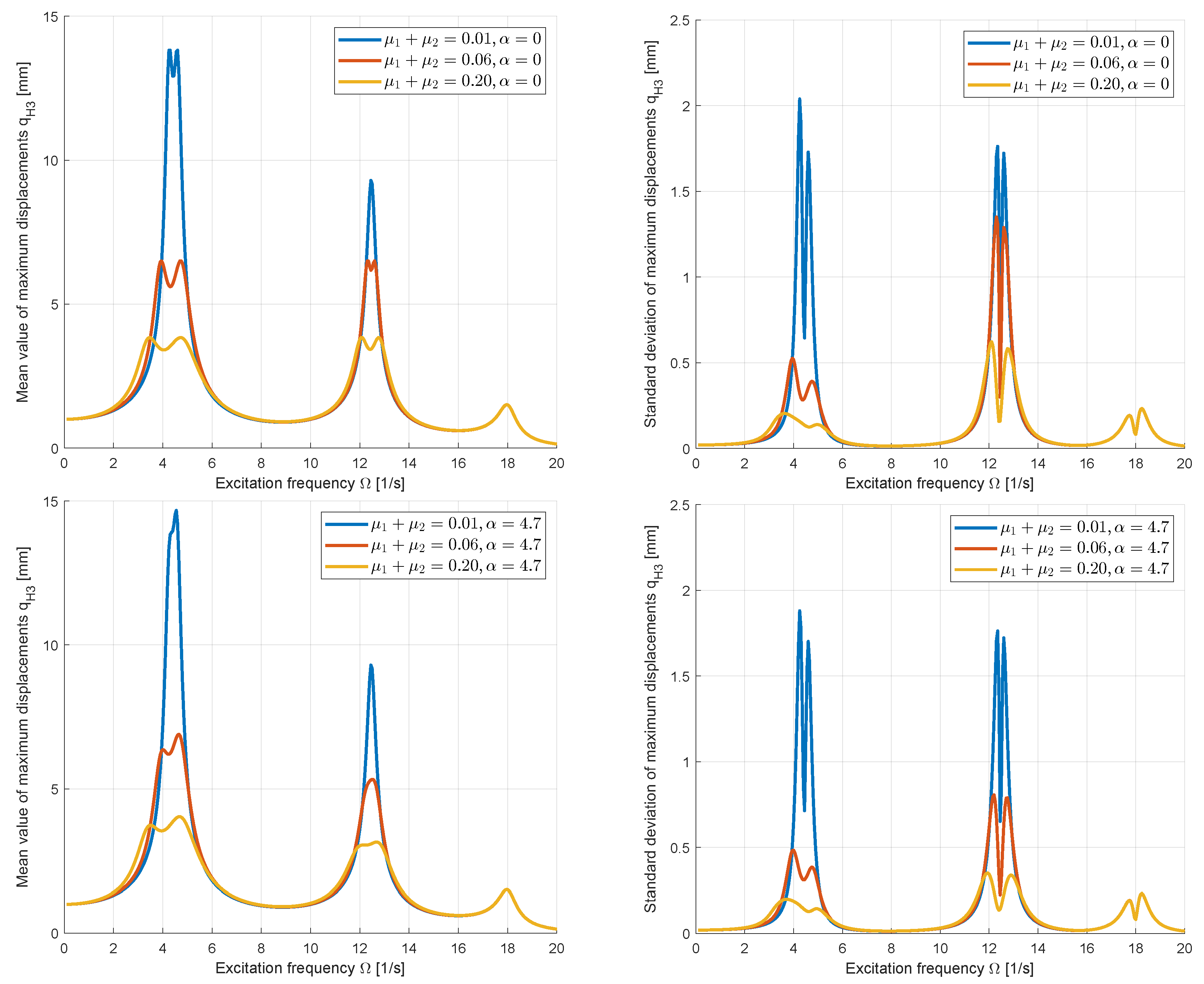
Figure 24.
Optimized maximum mean values and standard deviations of the maximum drift displacement of the third floor for an increasing mass of the TMDs and different safety margins
Figure 24.
Optimized maximum mean values and standard deviations of the maximum drift displacement of the third floor for an increasing mass of the TMDs and different safety margins
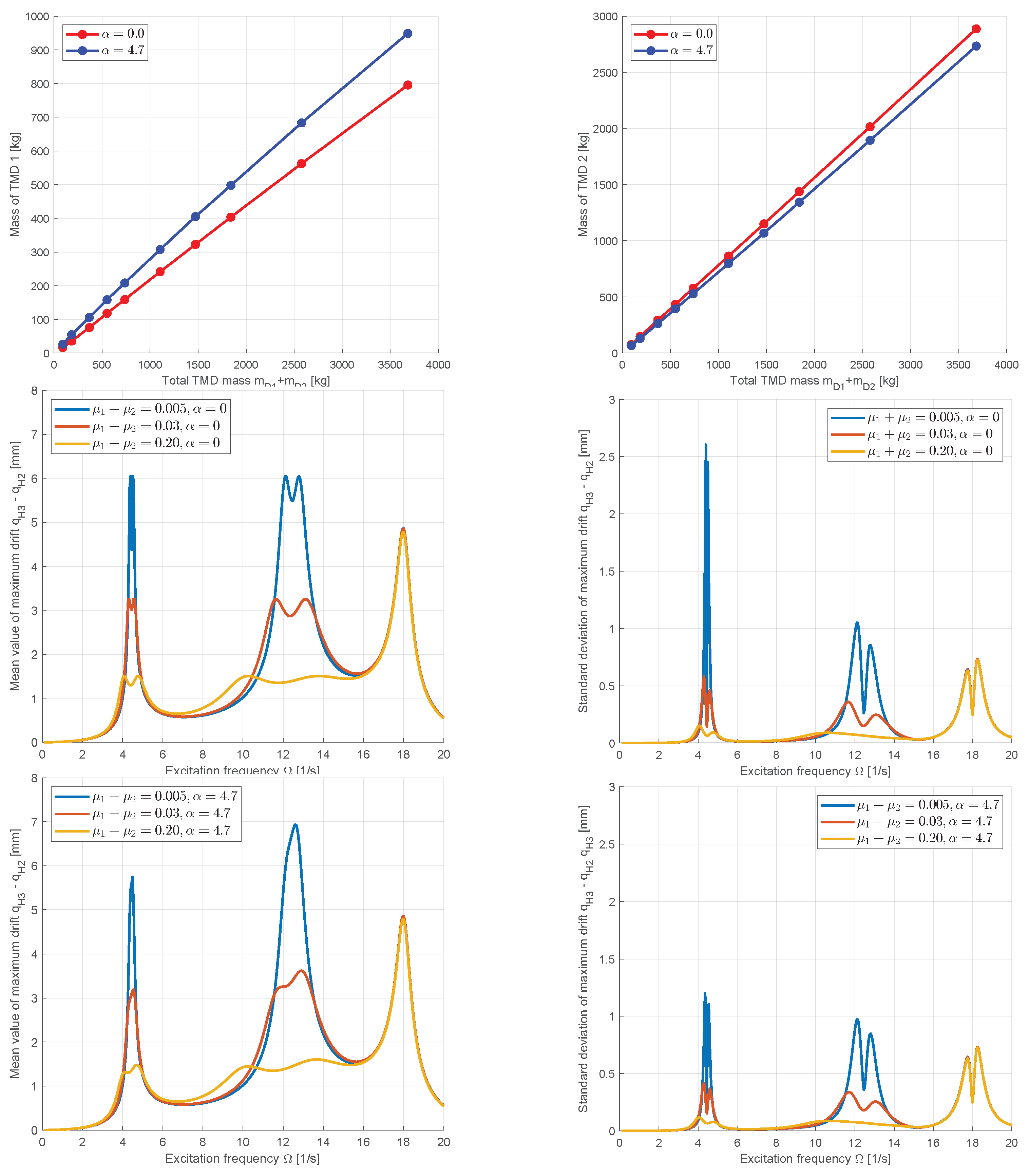

Table 1.
SDOF system with TMD: reference and optimization bounds and results of the single-objective optimization of
Table 1.
SDOF system with TMD: reference and optimization bounds and results of the single-objective optimization of
| Parameter | Unit | Reference | Den | Single-objective | Multi- | |
|---|---|---|---|---|---|---|
| Hartog | Bounds | Optimum | objective | |||
| kg | ||||||
| kN/m | ||||||
| - | ||||||
| - | - | |||||
| - | - | |||||
| - | - | |||||
Table 2.
Statistical properties of the scattering input parameters for the SDOF example with mean values according to the Den Hartog parameters
Table 2.
Statistical properties of the scattering input parameters for the SDOF example with mean values according to the Den Hartog parameters
| Parameter | Unit | Mean value | Coefficient of Variation | Distribution type |
|---|---|---|---|---|
| kg | Normal | |||
| kN/m | Normal | |||
| - | Normal | |||
| kg | Normal | |||
| kN/m | Normal | |||
| - | Normal |
Table 3.
Statistical properties of the input parameters for the MDOF example
| Parameter | Unit | Mean value | Coefficient of Variation | Distribution type |
|---|---|---|---|---|
| ,, | kg | Normal | ||
| ,, | kN/m | Normal | ||
| - | Normal | |||
| - | Normal | |||
| - | Normal | |||
| kg | Normal | |||
| kg | Normal | |||
| kN/m | Normal | |||
| kN/m | Normal | |||
| - | Normal | |||
| - | Normal |
Disclaimer/Publisher’s Note: The statements, opinions and data contained in all publications are solely those of the individual author(s) and contributor(s) and not of MDPI and/or the editor(s). MDPI and/or the editor(s) disclaim responsibility for any injury to people or property resulting from any ideas, methods, instructions or products referred to in the content. |
© 2025 by the authors. Licensee MDPI, Basel, Switzerland. This article is an open access article distributed under the terms and conditions of the Creative Commons Attribution (CC BY) license (http://creativecommons.org/licenses/by/4.0/).
Copyright: This open access article is published under a Creative Commons CC BY 4.0 license, which permit the free download, distribution, and reuse, provided that the author and preprint are cited in any reuse.


