
Submitted:
15 May 2025
Posted:
16 May 2025
You are already at the latest version
Abstract
Tuned Mass Damper Inerters (TMDIs) are recognized for their effectiveness in mitigating undesirable structural vibrations caused by unpredictable environmental loads. This study aims to derive closed-form expressions for the optimal parameters of a TMDI system using the principles of equal modal frequency and equal modal damping. The objective is to minimize the peak displacement and acceleration responses of a structure subjected to dynamic excitations. Four distinct strategies for controlling structural responses are presented. The resulting closed-form formulas are independent of the excitation frequency and depend solely on the structural damping and the mass ratio of the installed device. The proposed method is applied to a benchmark tall building subjected to wind excitation, demonstrating the robustness and effectiveness of the TMDI in enhancing structural performance. A key contribution of this study is the demonstration that significant reductions in structural displacement and acceleration responses can be achieved using a TMDI with a relatively low physical mass ratio. This finding highlights the efficiency and practicality of the proposed approach, especially for applications where adding large supplemental mass is impractical.
Keywords:
Tuned Mass Dampers
; Inerter
; Structural Control
; Equal modal Damping
; Equal modal Frequency
; Tall Buildings
; TMD
; TMDI
; Optimal
; Benchmark
1. Introduction to TMDI Damper
The rise of tall buildings has been a hallmark of modern urban development, driven by the need to optimize land use and accommodate growing populations [1,2,3,4,5]. As these structures have become increasingly slender and flexible, their susceptibility to wind-induced vibrations has emerged as a critical design challenge [6,7,8,9,10]. Particularly in buildings with rectangular floor plans, vortex shedding around sharp edges can induce significant oscillations in the across-wind direction, often resulting in higher peak floor accelerations than those caused by along-wind forces [1,11]. These accelerations can compromise occupant comfort, making their mitigation a key serviceability [12,13,14,15].
Efforts to suppress oscillatory motion in tall buildings began in the early 20th century, with the development of passive control strategies aimed at reducing displacements in the fundamental mode of vibration [9,15]. Among these, the Tuned Mass Damper (TMD) has proven to be one of the most effective and widely adopted solutions [16,17,18,19]. A TMD typically consists of a small auxiliary mass connected to the main structure via springs and dampers [8,20]. When properly tuned, the TMD resonates at the same frequency as the primary structure, allowing it to absorb vibratory energy and oscillate out of phase with the building, thereby reducing motion [18,20].
The theoretical foundation of TMD design is rooted in the fixed-point theory, which identifies an optimal damping condition where the system's response becomes independent of the structure’s inherent damping [21,22,23]. This theory has guided the development of numerous damping systems over the decades [23,24,25,26,27,28]. However, its applicability diminishes in structures with higher damping levels, where numerical methods are often required to accurately determine optimal parameters. It is well established that the tuning frequency and damping ratio of the TMD are critical to its effectiveness [21,22,27,28].
To further enhance vibration control, recent advancements have introduced the Tuned Mass-Damper-Inerter (TMDI) [4,7,22]. This system incorporates an inerter—a mechanical device that resists relative acceleration between its terminals, typically implemented using a flywheel mechanism [30,31,32]. The inerter amplifies the inertial effect of the attached mass, enabling greater vibration suppression without increasing the physical size of the damper [30]. Unlike traditional TMDs, which primarily target the fundamental mode, TMDIs can also influence higher vibration modes, which are particularly significant in tall buildings where multiple modes contribute to floor accelerations [22,26,27].
The objective of the present study is to derive closed-form solutions for the optimal design of TMDI systems in damped structures [27,28]. These solutions aim to be independent of the excitation frequency and based solely on the structural properties of the building. The study also compares the derived parameters with existing undamped models and evaluates the performance of TMDI-equipped tall buildings in mitigating displacement and acceleration responses under wind excitation [2,35,36]. A benchmark high-rise structure is used to assess the effectiveness of various TMDI configurations, with a focus on practical design considerations such as stroke length, inerter force magnitude, and device sizing [5,12,15,37,38,39,40].
2. The methodology of the Derivation of Optimum TMDI Parameters
Let m & be the mass of the main system and mass of TMDI, c & are damping of main system & TMD, whereas k & are stiffness of main system & TMDI respectively, while b is inerter mass (flywheel damper mass) connected to the base. The system parameters are defined as follows [29].
Figure 1.
TMDI System.
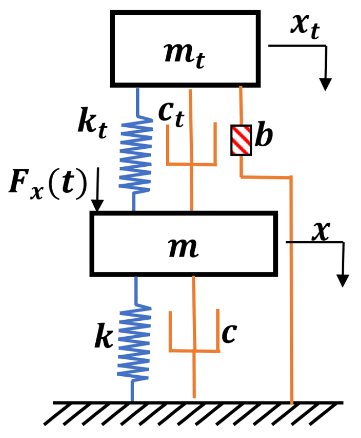
Where is the natural frequency of the main system; is the natural frequency of TMD; ξ is structural damping ratio; is damping ratio of TMD; is mass ratio and inerter-mass ratio, and is frequency ratio.
Using equations 1, equation 2 can be expressed in the term of system parameters, as equation 3.
The purpose of the state representation of the equation of motion is to condense the second-order ordinary differential equation into the form [17,49,50]
where 'z' represents the state vector and 'u' represents the input vector. The ‘ż’ and ‘A’ can be interpreted from equation 4. Here, 'A' and 'B' stand for the system matrix and input matrix, respectively. This general equation can be extended to TMD system matrices as indicated in equation 4, with 'M,' 'C,' and 'K' are mass, damping, and stiffness matrices, respectively [19,27,28]. The state matrix ‘A’ for equation 3 is expressed as equation 6,
3. Equal Modal Damping and Frequency of TMDI System
The Eigen solution in term of R of equation from equation 6 leads to the following characteristic polynomial as shown in equation 7 [24,26],
The solution of this polynomial results in 2 pairs of complex conjugates expressed as equation 8 [27,28].
Where, and , and are respectively modal frequency and modal damping of the first and second mode of vibration. The roots shown in equation (8), can be expressed as equation 9 as follow.
The expansion of equation 9 leads to equation 10.
Mathematically, equation 9 and equation 10 are the same equation but expressed in different system [28,29]. As per the equal modal damping & modal frequency hypothesis, means & , the equation (10) re-written as equation 11.
That means, the coefficient of equation 11 and equation 7 is the same, these proposals lead to the following equations 12 to 15 [28,29],
The natural frequency (), modal frequency (), and frequency ratio () have a non-negative value, hence, from equation 12, can be derived as,
Using equation 16 and equation 13, can be derived as,
It is to be noted that equations 16 and 17 represent complete closed-form presentation of equal modal damping ()and equal modal frequency (). Using equations 14 to 17, one can obtain equation 18 & 1).
By substituting in equation 19 using equation 18 and rearranging term it reduces into equation 20. Similarly, one can obtain equation 21, vice versa. Equations 20 and 21 are independent to and respectively, [28,29]. Both equations are simplified quartic equations and they have one pair of real and other one pair of complex conjugate roots. These expressions are independent of the optimum parameter, and they depend only on structural properties , and [28,29].
The roots of equation 20 are
Similarly, by using the factoring technique, roots of can also be summarized from equation 21 [28,29]
In equation 22 and 23, when inerter ratio , set equal to zero & upon the simplification it results from expression 24 and 25. This is a derivation of earlier work of authors [27,28].
Moreover, If the absolute mass ratio is taken as as sum of and , the equations 22 and 23 are presented as 26 and 27[28,29].
The solution of the quartic equation of and shows one pair of real & , & ) and other pair of the complex conjugate and , and . The and roots are commonly cited by various authors [8,22,25,27].
Here, optimal parameters, and show their presence in whole space, equation 26 and 27. The real roots and roots only because their partial presence in space. These roots are derived based on the proposed hypothesis for optimization given in [28,29], which produces , , and , the optimal real roots. The optimal parameters suggest that there are multiple solutions [27,28,29]. The equation 28 shows the optimal solution in a pair.
The following sections represent the graphical explanation and characteristic behaviors of optimal solutions.
4. Equal Modality on Optimal Parameters for TMDI
Figure 2 presents the root locus of the state matrix A, based on the characteristic polynomial of Equation 7[13,14,28,29]. Each real modal roots are tracked in terms of modal frequency and modal damping. Optimal parameters are identified when both fundamental modes exhibit equal modal damping and the first two modal frequencies align. Previous studies indicate that this condition termed natural parity yields optimal displacement and acceleration control, and improved structural performance [21,24,28]. In Figure 2(a), the vertical dash-dot line on the x-axis marks the two optimal real roots for damping; in Figure 2(b), it marks those for frequency.
Modal damping (blue, left y-axis) and modal frequency (red, right y-axis) are clearly distinguished. At the optimal state, the graph is divided into four horizontal dash-dot lines two for damping and two for frequency, each color-coded to its respective axis. All key parameter values are highlighted with matching-colored labels for clarity[13,14,28,29].
5. Effect of Absolute Mass Ratio for TMDI
Figure 3 illustrates the influence of the absolute mass ratio on various structural systems. As structural damping increases, the optimal frequency demand decreases for a given absolute mass ratio. This trend remains consistent when estimating equal modal frequencies, as shown in the inset of Figure 3(a). However, this trend reverses when evaluating equal modal damping at a constant absolute mass ratio but with reduced structural damping under these conditions, the optimal frequency demand is lower [13,14,29]. A similar reversal is observed for the optimal damping of a Tuned Mass Damper Inerter (TMDI), as shown in the inset of Figure 3(b).
The structural damping ratio and absolute mass ratio are independent but critical. Changes to either can cause sensitivity issues, as optimal tuning depends directly on both.
6. Procedure for Estimating Optimal Parameters in a TMDI Controlled Structure
The step-by-step procedure for estimating optimal parameters in a TMDI Controlled Structure is as follows:
- Estimate Natural Frequency: Using the stiffness and mass properties of the main system, estimate the natural frequency:
- Determine Mass and Damping Ratios: Evaluate Mass Ratio () and Inertance ratio based on the structural control strategy using TMDI. The Absolute Mass Ratio is calculated as . Determine Structural Damping Ratio (), as per the relevant standard.
- Calculate Optimal Frequency Ratio () using the equation 27, where /
- Compute Equal Modal Frequency (EMF) using equation 17:
- Estimate Optimal Damping Ratios , using equation 26,
- Calculate Equal Modal Damping (EMD) using equation 17: where,
- Determine Effective Optimal Damping Roots: The optimal damping roots are: .
- Proceed to Compute Parameters R₁ to R₄ as per equation 28.
7. Study of Benchmark Tall Building
The study involves a proposed 76-story building in Melbourne, Australia, with a height of 306.1 meters, although it was not [5,38,42,53]. Figure 4 illustrates the typical layout and elevation of the building, which measures 42 meters by 42 meters with chamfered corners and a slenderness ratio of 7.3, making it susceptible to wind loads. The structure features a reinforced concrete core at its center and a perimeter frame. The core is primarily designed to withstand wind loads, while the frame handles gravity and partial wind forces [15].
For the study, a discretized model was created by treating the columns and walls as Euler–Bernoulli beam elements, resulting in a giant cantilever beam model with 76 translational and 76 rotational degrees of freedom [3,5,12,38,53]. The first five mode shapes and corresponding natural period is shown in Figure 5.
Consequently, the proposed model, with 76 × 76 mass, damping, and stiffness matrices, is referred to as the 76-DOF model. The first five natural frequencies of the tall benchmark building are 0.16 Hz, 0.765 Hz, 1.992 Hz, 3.790 Hz, and 6.395 Hz.
This study investigates structural control using a passive TMDI system, where the inerter is grounded to enhance performance. The TMDI is strategically installed on the top floor of the structure to target and mitigate the first mode of vibration. Grounding the inerter end allows the system to capitalize on relative acceleration, thereby maximizing its damping effectiveness[13,14].
Previous research has demonstrated that inerters can achieve significant mass amplification—up to 3000 times the physical mass, with an average amplification of at least 100 times being commonly reported [13,14,48,54]. A variety of two-terminal inerter devices are commercially available, and configurations where one terminal is grounded have been advocated for improved performance [42,53,54].
To analyze the dynamic response of a wind-excited benchmark building equipped with the TMDI, a state-space approach is employed. The governing equations used for this analysis are presented in Section 2, specifically in Equations (4) and (5). The benchmark tall building has a total mass of 153,000 tons[3,5,12,46,53]. For the controlled structure, a 1% absolute mass ratio is considered for the passive control strategy.
8. Performance Measures of Benchmark Building
To assess the performance of the TMDI system, twelve response parameters are defined. represents the ratio of the root mean square (RMS) displacement at the 76th floor of the controlled structure to that of the uncontrolled structure, while denotes the corresponding ratio for RMS [14,19]. To capture the overall response across the structure, is defined as the average ratio of RMS displacements at selected target floors specifically floors 1,30,50, 55, 60, 65, 70, 75, and 76 of the controlled structure to those of the uncontrolled case, and similarly represents the average ratio of RMS accelerations at the same floors. Furthermore, quantifies the ratio of the maximum RMS displacement observed among the target floors of the controlled structure to the RMS displacement at the 76th floor of the uncontrolled [12,16]. Lastly, is defined as the ratio of the maximum RMS acceleration among the target floors of the controlled structure to the RMS acceleration at the 76th floor of the uncontrolled structure. These parameters collectively provide a comprehensive assessment of the TMDI's effectiveness in suppressing structural [11,13,14,29].
In addition to RMS, the peak response parameters are introduced to further evaluate the performance of the TMDI under extreme loading conditions. is defined as the ratio of peak displacement at the 76th floor of the controlled structure to that of the uncontrolled structure, while represents the corresponding ratio for peak acceleration response [12,55,56]. To capture the broader structural response, denotes the average ratio of peak displacements at selected target floors, specifically, floors 1, 30, 50, 55, 60, 65, 70, 75, and 76 between the controlled and uncontrolled structures. Similarly, is the average ratio of peak accelerations at these target floors. The parameter is defined as the ratio of the maximum peak displacement observed among the target floors of the controlled structure to the peak displacement at the 76th floor of the uncontrolled structure. Lastly, quantifies the ratio of the maximum peak acceleration among the target floors of the controlled structure to the peak displacement at the 76th floor of the uncontrolled structure. Together, these parameters provide a comprehensive view of the TMDI’s capability to limit both sustained and extreme structural [13,14,29,43].
9. Assessment of Structural Response Characteristics
Table 1 presents a comparative assessment of the structural response under four different root configurations, to , using both RMS and peak response indicators. The parameter shows that achieves the highest reduction at 46.7%, followed closely by at 46.4%, at 45.0%, and at 44.5%. Similarly, the RMS acceleration reduction, indicated by , is most significant for at 64.1%, followed by at 63.9%, at 60.9%, and at 60.5% [12].
The parameters and shows the superior performance of , although with a marginal advantage over . Moreover, and remain consistent between and , indicating robust control effectiveness in both configurations[28,29].
In terms of peak response, the reduction in peak displacement at the 76th floor, as shown by , is 30.4% for , 29.0% for , 25.6% for , and 22.7% for . This trend mirrors the performance of the RMS indicators and highlights as the most effective configuration across both response categories. The corresponding peak acceleration values shown by follow a similar pattern, with again yielding the lowest response ratio at 0.453[12,16,29]. For more detail, refer Table 2.
Additional parameters through consistently indicate a gradual decline in performance from to . Specifically, and show the average peak displacement and acceleration ratios increasing slightly across the roots, while and reflect the highest localized peak responses within the structure[1,3,19,43], as shown in Table 3.
10. System Response Evaluation and Insight
Figure 6 and Figure 7 present the displacement and acceleration time histories of R₁ across various floor levels, under 0% stiffness uncertainty. These responses are overlaid with those of the uncontrolled structure for direct comparison over the full-time frame.
A key observation is that the passive TMDI controller maintains effective control throughout the entire duration, at no point it loses stability or effectiveness. The Figure 6 and Figure 7 clearly demonstrate a significant reduction in both displacement and acceleration, as annotated in the figure captions peak response [4,13,14,28,29].
Moreover, the TMDI stroke behavior remains smooth and stable, with no abrupt swings in either displacement or acceleration. This indicates a well-tuned system that not only suppresses structural response effectively but also operates within practical stroke limits, an essential consideration for real-world implementation [3,18,28].
The analysis clearly shows that root configuration delivers the most effective vibration mitigation, achieving the greatest reductions in both RMS and peak structural responses. Notably, this high level of performance is achieved with a relatively low mass ratio, underscoring the efficiency of the proposed TMDI design[3,4,14,29,43]. Root configurations through show progressively reduced performance, suggesting that careful tuning of TMDI parameters, particularly those associated with modal frequency and damping alignment, is critical for maximizing structural control. Overall, the results confirm the robustness and practicality of the TMDI system, especially under wind-induced excitations in tall buildings. The offers moderate but reliable control performance [27,28].
The evaluation of stiffness uncertainty across 12 performance metrics (P₁–P₁₂) reveals critical insights into the sensitivity and robustness of controlled structural systems, refer Table 4 in association with table 1[12,56]. These parameters, which capture both RMS and peak responses in terms of displacement and acceleration, highlight the impact of ±10% variations in structural stiffness, the graphics is presented in Figure 8 and Figure 9.
Notably, under 0% stiffness uncertainty conditions, all four root configurations (R₁ to R₄) yield substantial performance benefits, with reductions exceeding 40–60% across most parameters. For example, R₁ and R₂ consistently achieve RMS displacement and acceleration reductions around 47–64% at the 76th floor (P₁ and P₂), underscoring their effectiveness in mitigating dynamic responses.
However, as stiffness increases by 10%, performance degrades significantly across all configurations, Further insights can be observed in Figure 8 and Figure 9, which provide additional clarity and depth to the analysis. This degradation is most prominent in R₃ and R₄, where several parameters approach or even exceed unity (e.g., R₃’s P₇ = 1.093 and R₄’s P₇ = 1.084), indicating that the controlled structure performs worse than the uncontrolled case in terms of peak displacement, refer to Table 4 in conjunction with Table 1, for a comparative understanding of the results and parameter relationships. This suggests that overestimating stiffness not only reduces the damping efficiency of the control system but can potentially lead to control-structure interaction issues, where the tuned mass dampers (TMDIs) become detuned from the dominant modal frequencies[12,13,14,16]. This mismatch exacerbates peak responses rather than suppressing them.
In contrast, as stiffness decreases by 10%, generally preserves the effectiveness of the control strategies and, in some cases, even improves it slightly. For instance, R₃ sees P₁ drop to 0.468 (a 53.2% reduction), indicating enhanced performance under reduced stiffness. This suggests that a slight underestimation of stiffness keeps the TMDI closer to resonance with the structural modes, thus maintaining or boosting damping effectiveness. Yet, this benefit does not uniformly extend across all metrics or configurations, revealing the complex interplay between structural properties and controller dynamics.
Figure 10.
Effect of ±10% Stiffness Variation (K) on RMS and Peak Responses of R₁–R₄ Across Benchmark Building Levels vs. Uncontrolled Structure.
Figure 10.
Effect of ±10% Stiffness Variation (K) on RMS and Peak Responses of R₁–R₄ Across Benchmark Building Levels vs. Uncontrolled Structure.
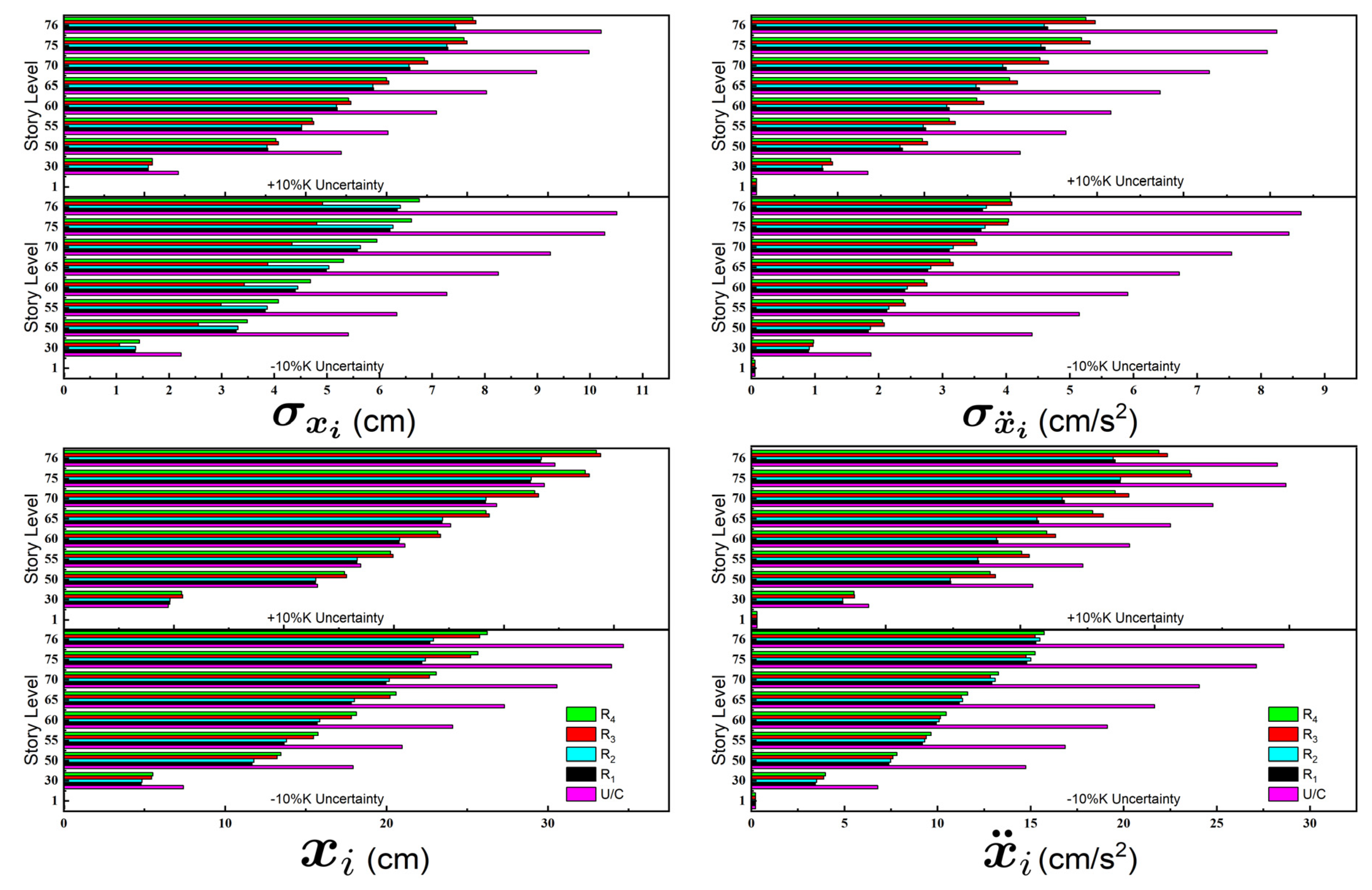
Furthermore, RMS-based parameters (P₁–P₆) appear more sensitive to stiffness uncertainty than peak response parameters (P₇–P₁₂), particularly in R₃ and R₄, where peak responses degrade sharply under positive stiffness deviations. This divergence implies that control schemes optimized for average energy dissipation may not necessarily perform well under extreme transient loads. Therefore, the data strongly advocate for robust control strategies that can maintain stability and performance across reasonable stiffness variations[13,14,28,29]. Among the four configurations, R₁ and R₂ stand out as the most resilient to uncertainty, maintaining consistent reductions across all 12 parameters and avoiding the counterproductive amplification seen in R₃ and R₄ under high-stiffness conditions.
In summary, this analysis reveals that stiffness uncertainty, especially positive deviation, can critically undermine structural control performance, sometimes reversing intended benefits. It underscores the necessity of designing controllers that are not only optimal under nominal conditions but also robust to structural variability, particularly in tall or flexible buildings where stiffness is prone to estimation error or time-dependent change[27,28,29]. The conclusion necessitates a comprehensive reassessment of the system's time-domain responses through their transformation into the frequency domain. Particular attention should be directed toward the region surrounding the peak response, where subtle, microscopic variations may hold critical significance. Such focused analysis will offer a more robust foundation for validating the conclusion and enhancing its credibility.
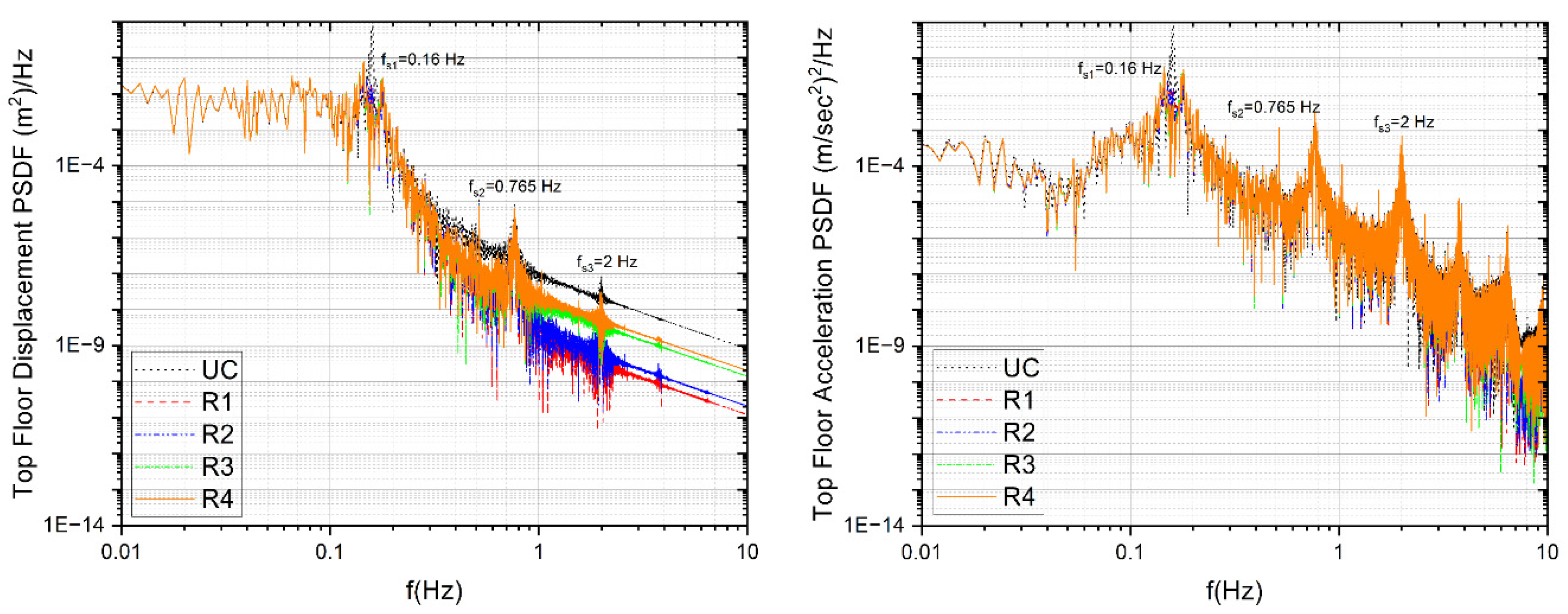
The Figure 11 present Power Spectral Density Functions (PSDFs) of top floor displacement and acceleration for a structural system subjected to dynamic loading, comparing uncontrolled (UC) and various controlled scenarios (R₁– R₄). The three natural frequencies of the structure - 0.16 Hz, 0.765 Hz, and 2 Hz - are evident as peaks in the PSDF plots. The control strategies aim to suppress structural response at these resonant frequencies. Among the cases, R₁ consistently delivers the most effective reduction in both displacement and acceleration PSDFs across all modes, indicating superior performance in mitigating structural vibrations. R₂ and R₃ also perform well, though slightly less effective than R₁. In contrast, R₄ shows limited suppression and in some frequency, ranges even amplify the acceleration response, suggesting poor tuning or instability. Overall, R₁ emerges as the most efficient control strategy, achieving significant response reduction and enhanced dynamic stability.
Figure 11.
Power Spectral Density Function (PSDF) at the Top Floor without uncertainity: (a) Displacement Response; (b) Acceleration Response.
Figure 11.
Power Spectral Density Function (PSDF) at the Top Floor without uncertainity: (a) Displacement Response; (b) Acceleration Response.
The time-domain plots shown in Figure 12, illustrate the top floor displacement and acceleration responses of a structure controlled using four different strategies (R₁– R₄), all with the same mass ratio. The displacement response, shown on the left, and the acceleration response, on the right, both include zoomed-in views between 500 and 600 seconds to highlight differences in control performance. Across the full simulation period, R₁ and R₂ demonstrate consistently lower displacement amplitudes compared to R₃ and R₄, indicating more effective vibration suppression.
In the magnified section, R₁ and R₂ continue to exhibit smoother and more controlled behavior, while R₃ and particularly R₁ display more irregular and amplified motion. Similarly, in the acceleration response, R₁ maintains the lowest fluctuation levels, suggesting better dynamic control. R₄, in contrast, shows the largest acceleration variations, reinforcing its comparatively poorer performance. These results align with the frequency-domain analysis, confirming that R₁ delivers the most stable and efficient control among the four strategies.
Figure 12 illustrates the time-domain responses at the top floor, specifically analyzing the TMDI behavior across control strategies R₁ through R₄, all employing an identical mass ratio. The left-hand graphs depict displacement, while the right-hand ones show acceleration, each accompanied by zoomed-in views to highlight detailed temporal effects. Of all the strategies, R₄ demonstrates the most pronounced and persistent oscillations in both displacement and acceleration - especially evident in the focused intervals (560–660 sec for displacement and approximately 540–600 sec for acceleration) - indicating excessive TMD activity and potential instability. In contrast, R₁ and R₂ consistently exhibit lower amplitude responses and smoother profiles, suggesting more effective TMD stroke regulation and superior energy dissipation. The acceleration curve for R₄ features abrupt, irregular spikes, further underscoring its limited control capability. These results collectively affirm that R₁ and R₂ offer the most reliable performance in minimizing TMD stroke and enhancing system stability, while R₄’s behavior raises concerns about its suitability. For a comprehensive understanding of TMD stroke, please refer to Figure 6 and Figure 7. Additionally, the RMS and Peak values of the strokes can be found in the last row of the respective tables for detailed analysis.
11. Conclusion
This study offers a comprehensive assessment of four Tuned Mass Damper Inerter (TMDI) configurations R₁ to R₄ for controlling wind-induced vibrations in tall buildings. R₁ consistently demonstrates superior performance, achieving the most substantial reductions in both displacement and acceleration across key structural modes, as revealed by frequency-domain PSDF analysis. Time-domain evaluations further affirm R₁’s and R₂’s effectiveness, with smooth, low-amplitude responses and stable TMDI stroke behavior, indicating efficient energy dissipation. In contrast, R₄ performs poorly, often amplifying responses and exhibiting erratic motion, pointing to instability and inadequate tuning. Quantitative metrics (P₁–P₁₂) highlights R₁'s ability to reduce RMS acceleration by up to 64.1% and peak displacement by 30.4%, maintaining top performance across various structural levels. Sensitivity analysis reveals that stiffness variability, especially an increase of 10%, degrades R₃ and R₄’s effectiveness, underscoring the need for robust tuning. Overall, R₁ emerges as the most practical and resilient TMDI solution, with R₂ as a viable secondary option, while R₄ poses control risks due to instability and sensitivity to structural uncertainties. The most significant contribution of this work lies in its control strategy, which is based on the absolute mass ratio, a combination of the physical mass ratio of the TMD and the virtual mass ratio generated by the inerter. This means that when the inerter is inactive (i.e., inertance is zero), the TMD must weigh approximately 1530 tons to achieve the desired control. However, when the inerter operates at full capacity, it can generate an equivalent inertial effect of 1530 tons.
Given that inerters typically offer a mass amplification factor of around 100, a physical mass of just 15 tons can produce the same control effect. This breakthrough suggests a transformative potential for the future of structural control in tall buildings especially for mitigating wind-induced vibrations by enabling effective control with minimal physical mass. This realization brings engineers closer to a long-standing aspiration: achieving high-performance structural control without the burden of massive added weight.
Author Contributions
The principal author, was responsible for conceptualization, methodology, software development, validation, formal analysis, investigation, resource management, data curation, original draft preparation, visualization, supervision, and project administration. also led the writing and editing of the manuscript and ensured the integrity and accuracy of the research. The second author, served as the supervisor of the project. contributed to the review of the study, participated in the validation process, and also provided critical review and editing support during the manuscript preparation. All authors have read and agreed to the published version of the manuscript.
Funding
This research received no external funding.
Data Availability Statement
The research data supporting the findings of this study are available from the corresponding author upon reasonable request.
Conflicts of Interest
The authors declare no conflicts of interest.
Abbreviations
The following abbreviations are used in this manuscript:
| TMD | Tuned Mass Damper |
| TMDI | Tune Mass Damper Inerter |
| SDOF | Single Degree Of Freedom |
| MDOF | Multi Degree Of Freedom |
| EMF | Equal Modal Frequency |
| EMD | Equal Modal Damping |
| PSDFs | Power Spectral Density Functions |
| UC | Uncontrolled Structures |
| RMS | Root M |
References
- Taranath, B.S. Wind and Earthquake Resistant Buildings; 0 ed.; CRC Press, 2004; ISBN 978-0-8493-3809-0.
- Simiu, E.; Yeo, D. Wind Effects on Structures: Modern Structural Design for Wind; Fourth edition.; John Wiley & Sons: Hoboken, NJ, 2019; ISBN 978-1-119-37593-7. [Google Scholar]
- Elias, S.; Matsagar, V. Research Developments in Vibration Control of Structures Using Passive Tuned Mass Dampers. Annu. Rev. Control 2017, 44, 129–156. [Google Scholar] [CrossRef]
- Giaralis, A.; Petrini, F. Wind-Induced Vibration Mitigation in Tall Buildings Using the Tuned Mass-Damper-Inerter. J. Struct. Eng. 2017, 143, 04017127. [Google Scholar] [CrossRef]
- Samali, B.; Kwok, K.C.S.; Wood, G.S.; Yang, J.N. Wind Tunnel Tests for Wind-Excited Benchmark Building. J. Eng. Mech. 2004, 130, 447–450. [Google Scholar] [CrossRef]
- Frahm, H. Device for Damping Vibrations of Bodies 1911.
- Hartog, J.P.D. Mechanical Vibrations; Courier Corporation, 1985; ISBN 978-0-486-64785-2.
- Sadek, F.; Mohraz, B.; Taylor, A.W.; Chung, R.M. A METHOD OF ESTIMATING THE PARAMETERS OF TUNED MASS DAMPERS FOR SEISMIC APPLICATIONS. Earthq. Eng. Struct. Dyn. 1997, 26, 617–635. [Google Scholar] [CrossRef]
- Structural Motion Engineering; ISBN 978-3-319-06281-5.
- Design Optimization of Active and Passive Structural Control Systems:; Lagaros, N.D., Plevris, V., Mitropoulou, C.C., Eds.; IGI Global, 2013; ISBN 978-1-4666-2029-2.
- Xu, K.; Dai, Q.; Bi, K.; Fang, G.; Ge, Y. Closed-form Design Formulas of TMDI for Suppressing Vortex-induced Vibration of Bridge Structures. Struct. Control Health Monit. 2022, 29. [Google Scholar] [CrossRef]
- Suthar, S.J.; Jangid, R.S. Design of Tuned Liquid Sloshing Dampers Using Nonlinear Constraint Optimization for Across-Wind Response Control of Benchmark Tall Building. Structures 2021, 33, 2675–2688. [Google Scholar] [CrossRef]
- Islam, N.U.; Jangid, R.S. Optimum Parameters of Tuned Inerter Damper for Damped Structures. J. Sound Vib. 2022, 537, 117218. [Google Scholar] [CrossRef]
- Prakash, S.; Jangid, R.S. Optimum Parameters of Tuned Mass Damper-Inerter for Damped Structure under Seismic Excitation. Int. J. Dyn. Control 2022, 10, 1322–1336. [Google Scholar] [CrossRef]
- Pisal, A.Y.; Jangid, R.S. Dynamic Response of Structure with Tuned Mass Friction Damper. Int. J. Adv. Struct. Eng. 2016, 8, 363–377. [Google Scholar] [CrossRef]
- Suthar, S.J.; Patil, V.B.; Jangid, R.S. Optimization of MR Dampers for Wind-Excited Benchmark Tall Building. Pract. Period. Struct. Des. Constr. 2022, 27, 04022048. [Google Scholar] [CrossRef]
- Paz, M.; Kim, Y.H. Structural Dynamics: Theory and Computation; Springer, 2018; ISBN 978-3-319-94743-3.
- Hart, G.C.; Wong, K. Structural Dynamics for Structural Engineers; John Wiley & Sons: New York Weinheim, 2000; ISBN 978-0-471-36169-5. [Google Scholar]
- Connor, J.; Laflamme, S. Structural Motion Engineering; Springer International Publishing: Cham, 2014; ISBN 978-3-319-06280-8. [Google Scholar]
- Rao, S.S. Mechanical Vibrations; Addison-Wesley, 1990; ISBN 978-0-201-50156-8.
- Warburton, G.B. Optimum Absorber Parameters for Various Combinations of Response and Excitation Parameters. Earthq. Eng. Struct. Dyn. 1982, 10, 381–401. [Google Scholar] [CrossRef]
- Villaverde, R. Reduction Seismic Response with Heavily-Damped Vibration Absorbers. Earthq. Eng. Struct. Dyn. 1985, 13, 33–42. [Google Scholar] [CrossRef]
- Sladek, J.R.; Klingner, R.E. Effect of Tuned-Mass Dampers on Seismic Response. J. Struct. Eng. 1983, 109, 2004–2009. [Google Scholar] [CrossRef]
- Jacquot, R.G. Optimal Dynamic Vibration Absorbers for General Beam Systems. J. Sound Vib. 1978, 60, 535–542. [Google Scholar] [CrossRef]
- Miranda, J.C. A Method for Tuning Tuned Mass Dampers for Seismic Applications. Earthq. Eng. Struct. Dyn. 2013, 42, 1103–1110. [Google Scholar] [CrossRef]
- Miranda, J.C. System Intrinsic, Damping Maximized, Tuned Mass Dampers for Seismic Applications. Struct. Control Health Monit. 2012, 19, 405–416. [Google Scholar] [CrossRef]
- Thakur, V.M.; Jaiswal, O.R. Optimum Parameters of Variant Tuned Mass Damper Using Equal Eigenvalue Criterion. Earthq. Eng. Struct. Dyn. 2023, 52, 2852–2860. [Google Scholar] [CrossRef]
- Patel, V.B.; Jangid, R.S. Closed-Form Derivation of Optimum Tuned Mass Damper Parameter Based on Modal Multiplicity Criteria. ASPS Conf. Proc. 2022, 1, 1041–1049. [Google Scholar] [CrossRef]
- Patel, V.B.; Jangid, R.S. Optimal Parameters for Tuned Mass Dampers and Examination of Equal Modal Frequency and Damping Criteria. J. Vib. Eng. Technol. 2024, 12, 7159–7173. [Google Scholar] [CrossRef]
- Marian, L.; Giaralis, A. Optimal Design of a Novel Tuned Mass-Damper–Inerter (TMDI) Passive Vibration Control Configuration for Stochastically Support-Excited Structural Systems. Probabilistic Eng. Mech. 2014, 38, 156–164. [Google Scholar] [CrossRef]
- Papageorgiou, C.; Smith, M.C. Laboratory Experimental Testing of Inerters. In Proceedings of the Proceedings of the 44th IEEE Conference on Decision and Control; IEEE: Seville, Spain, 2005; pp. 3351–3356. [Google Scholar]
- Scheibe, F.; Smith, M.C. Analytical Solutions for Optimal Ride Comfort and Tyre Grip for Passive Vehicle Suspensions. Veh. Syst. Dyn. 2009, 47, 1229–1252. [Google Scholar] [CrossRef]
- Schmitz, T.L.; Smith, K.S. Mechanical Vibrations: Modeling and Measurement; Springer International Publishing: Cham, 2021; ISBN 978-3-030-52343-5. [Google Scholar]
- Barredo, E.; Blanco, A.; Colín, J.; Penagos, V.M.; Abúndez, A.; Vela, L.G.; Meza, V.; Cruz, R.H.; Mayén, J. Closed-Form Solutions for the Optimal Design of Inerter-Based Dynamic Vibration Absorbers. Int. J. Mech. Sci. 2018, 144, 41–53. [Google Scholar] [CrossRef]
- Brzeski, P.; Pavlovskaia, E.; Kapitaniak, T.; Perlikowski, P. The Application of Inerter in Tuned Mass Absorber. Int. J. Non-Linear Mech. 2015, 70, 20–29. [Google Scholar] [CrossRef]
- Hou, F.; Jafari, M. Investigation Approaches to Quantify Wind-Induced Load and Response of Tall Buildings: A Review. Sustain. Cities Soc. 2020, 62, 102376. [Google Scholar] [CrossRef]
- Kikuchi, H.; Tamura, Y.; Ueda, H.; Hibi, K. Dynamic Wind Pressures Acting on a Tall Building Model — Proper Orthogonal Decomposition. J. Wind Eng. Ind. Aerodyn. 1997, 69–71, 631–646. [Google Scholar] [CrossRef]
- Wang, L.; Nagarajaiah, S.; Shi, W.; Zhou, Y. Study on Adaptive-passive Eddy Current Pendulum Tuned Mass Damper for Wind-induced Vibration Control. Struct. Des. Tall Spec. Build. 2020, 29, e1793. [Google Scholar] [CrossRef]
- Taha, A.E. Vibration Control of a Tall Benchmark Building under Wind and Earthquake Excitation. Pract. Period. Struct. Des. Constr. 2021, 26, 04021005. [Google Scholar] [CrossRef]
- Zhang, Y.; Li, L.; Guo, Y.; Zhang, X. Bidirectional Wind Response Control of 76-Story Benchmark Building Using Active Mass Damper with a Rotating Actuator. Struct. Control Health Monit. 2018, 25, e2216. [Google Scholar] [CrossRef]
- Yang, J.N.; Agrawal, A.K.; Samali, B.; Wu, J.-C. Benchmark Problem for Response Control of Wind-Excited Tall Buildings. J. Eng. Mech. 2004, 130, 437–446. [Google Scholar] [CrossRef]
- Ma, R.; Bi, K.; Hao, H. Inerter-Based Structural Vibration Control: A State-of-the-Art Review. Eng. Struct. 2021, 243, 112655. [Google Scholar] [CrossRef]
- Wagg, D.J. A Review of the Mechanical Inerter: Historical Context, Physical Realisations and Nonlinear Applications. Nonlinear Dyn. 2021, 104, 13–34. [Google Scholar] [CrossRef]
- Ma, H.; Cheng, Z.; Jia, G.; Shi, Z. Energy Analysis of an Inerter-enhanced Floating Floor Structure (In-FFS) under Seismic Loads. Earthq. Eng. Struct. Dyn. 2022, 51, 3111–3130. [Google Scholar] [CrossRef]
- Kaveh, A.; Fahimi Farzam, M.; Hojat Jalali, H. Statistical Seismic Performance Assessment of Tuned Mass Damper Inerter. Struct. Control Health Monit. 2020, 27. [Google Scholar] [CrossRef]
- Hu, Y.; Chen, M.Z.Q.; Shu, Z.; Huang, L. Analysis and Optimisation for Inerter-Based Isolators via Fixed-Point Theory and Algebraic Solution. J. Sound Vib. 2015, 346, 17–36. [Google Scholar] [CrossRef]
- Li, D.; Ikago, K. Optimal Design of Nontraditional Tuned Mass Damper for Base-Isolated Building. J. Earthq. Eng. 2023, 27, 2841–2862. [Google Scholar] [CrossRef]
- Krenk, S. Resonant Inerter Based Vibration Absorbers on Flexible Structures. J. Frankl. Inst. 2019, 356, 7704–7730. [Google Scholar] [CrossRef]
- Shi, B.; Yang, J.; Jiang, J.Z. Tuning Methods for Tuned Inerter Dampers Coupled to Nonlinear Primary Systems. Nonlinear Dyn. 2022, 107, 1663–1685. [Google Scholar] [CrossRef]
- Paz, M.; Kim, Y.H. Structural Dynamics: Theory and Computation; Springer International Publishing: Cham, 2019; ISBN 978-3-319-94742-6. [Google Scholar]
- Chopra, A.K. Dynamics of Structures: Theory and Applications to Earthquake Engineering; Pearson Always learning; Fifth edition.; Pearson: Hoboken, NJ, 2017; ISBN 978-0-13-455512-6. [Google Scholar]
- SSTL : Structural Control Benchmarks. Available online: https://sstl.cee.illinois.edu/benchmarks/ (accessed on 4 May 2025).
- Kang, J.; Ikago, K. Seismic Control of Multidegree-of-freedom Structures Using a Concentratedly Arranged Tuned Viscous Mass Damper. Earthq. Eng. Struct. Dyn. 2023, 52, 4708–4732. [Google Scholar] [CrossRef]
Figure 2.
Equal modal damping and frequency effect for TMDI for a) optimal damping b) optimal frequency.
Figure 2.
Equal modal damping and frequency effect for TMDI for a) optimal damping b) optimal frequency.
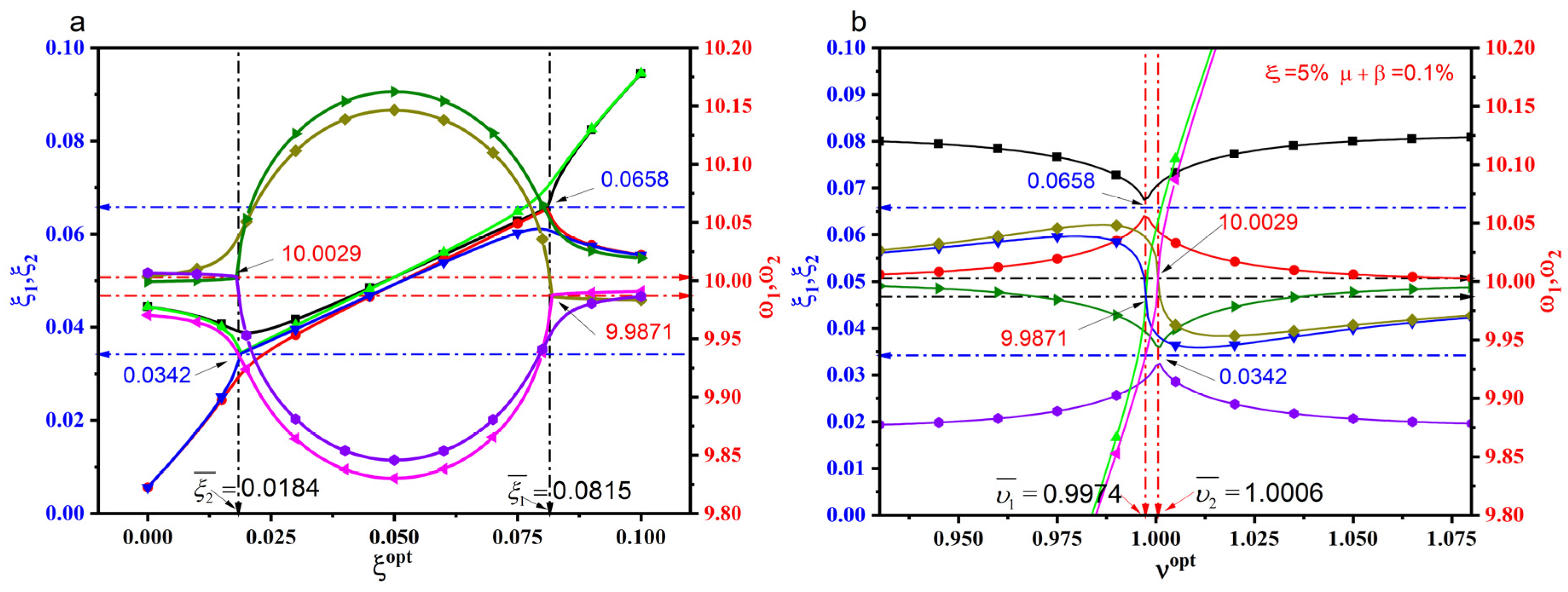
Figure 3.
Variation in optimal frequency and EMD against absolute mass ratio.
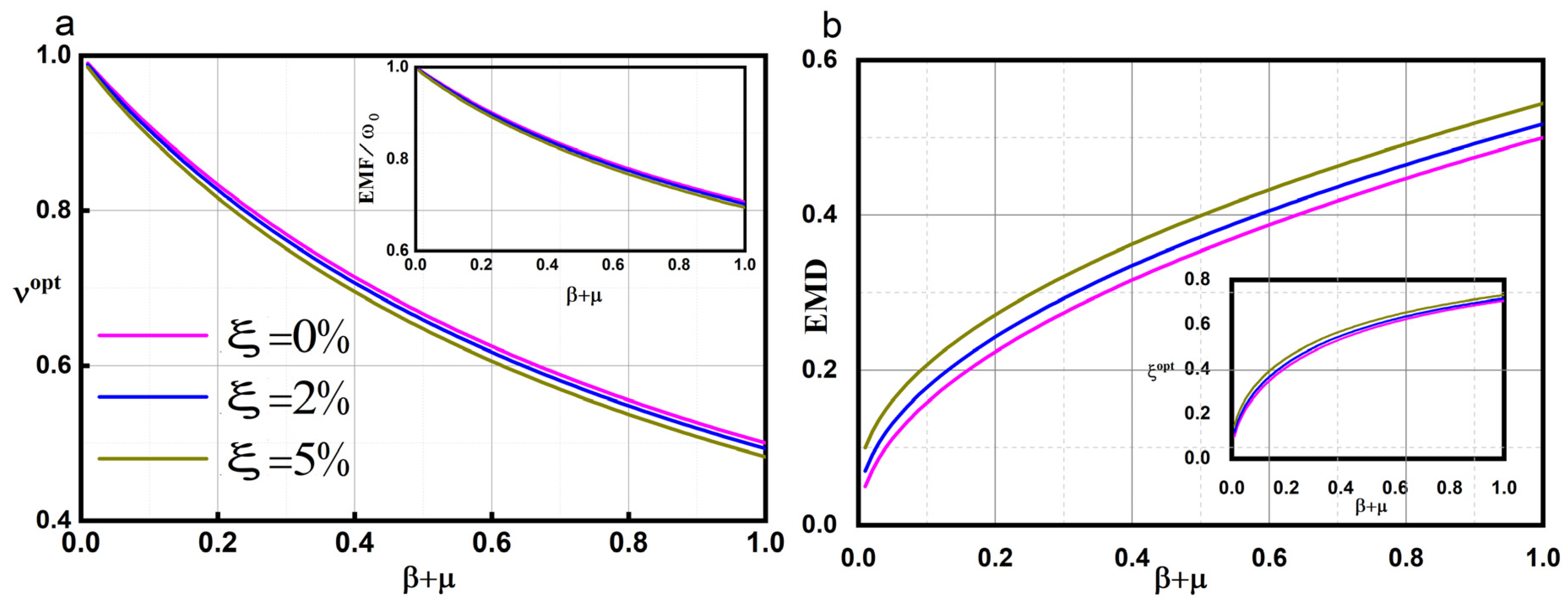
Figure 4.
Benchmark Building a) Typical floor plan b) Elevation.
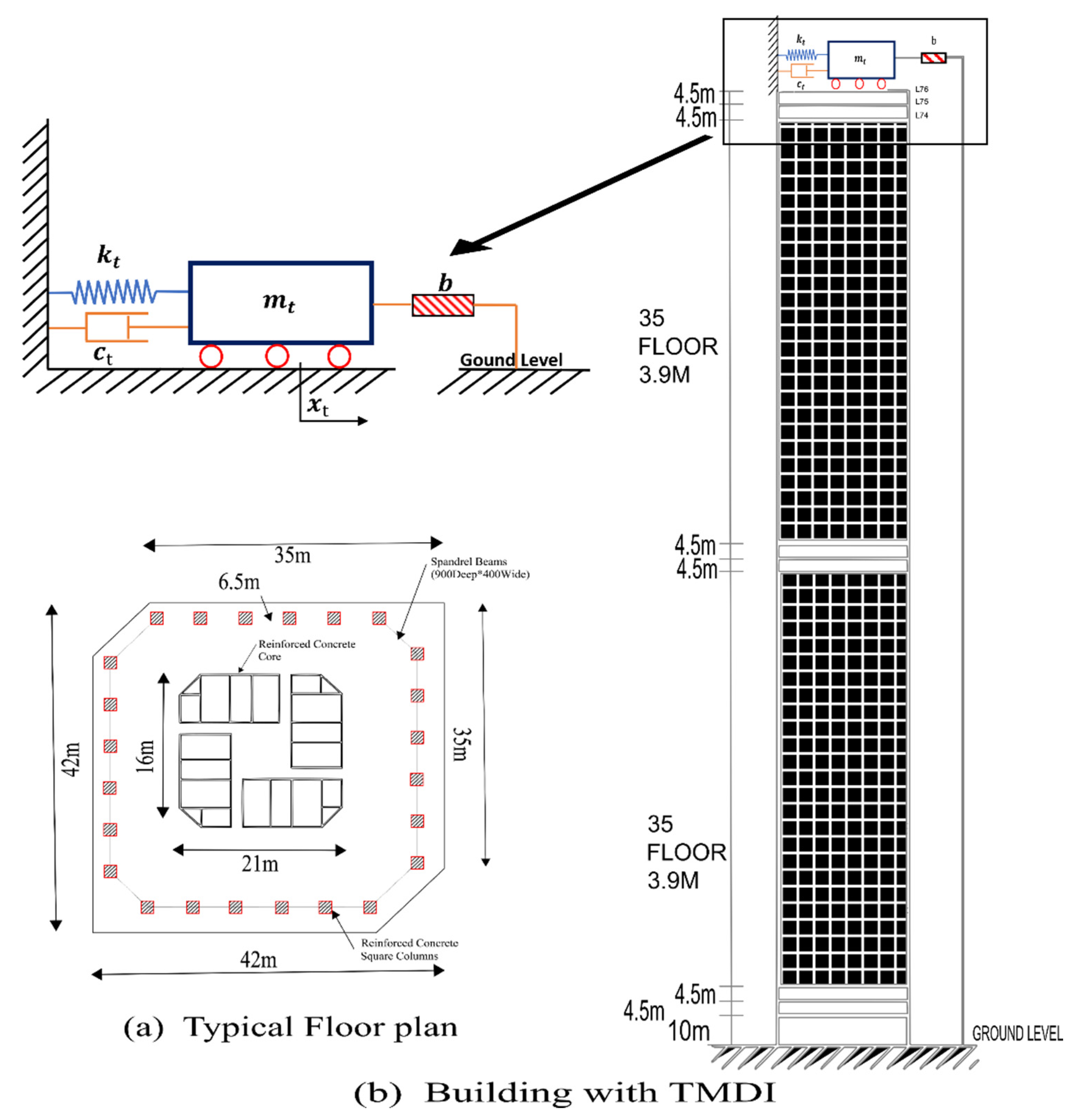
Figure 5.
Mode shapes of buildings.
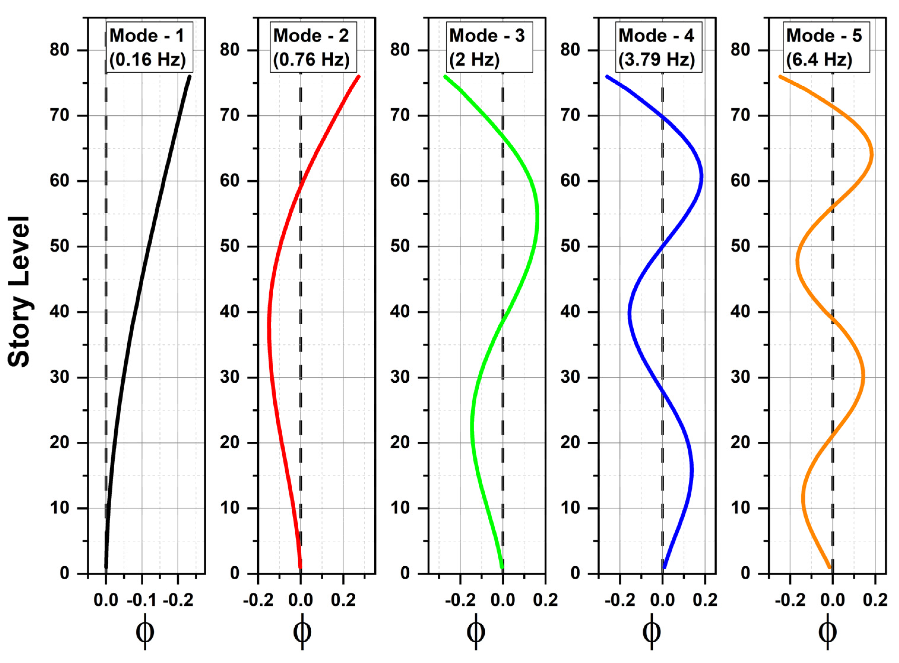
Figure 6.
Displacement Response Time History for R₁ at Various Floor Levels.
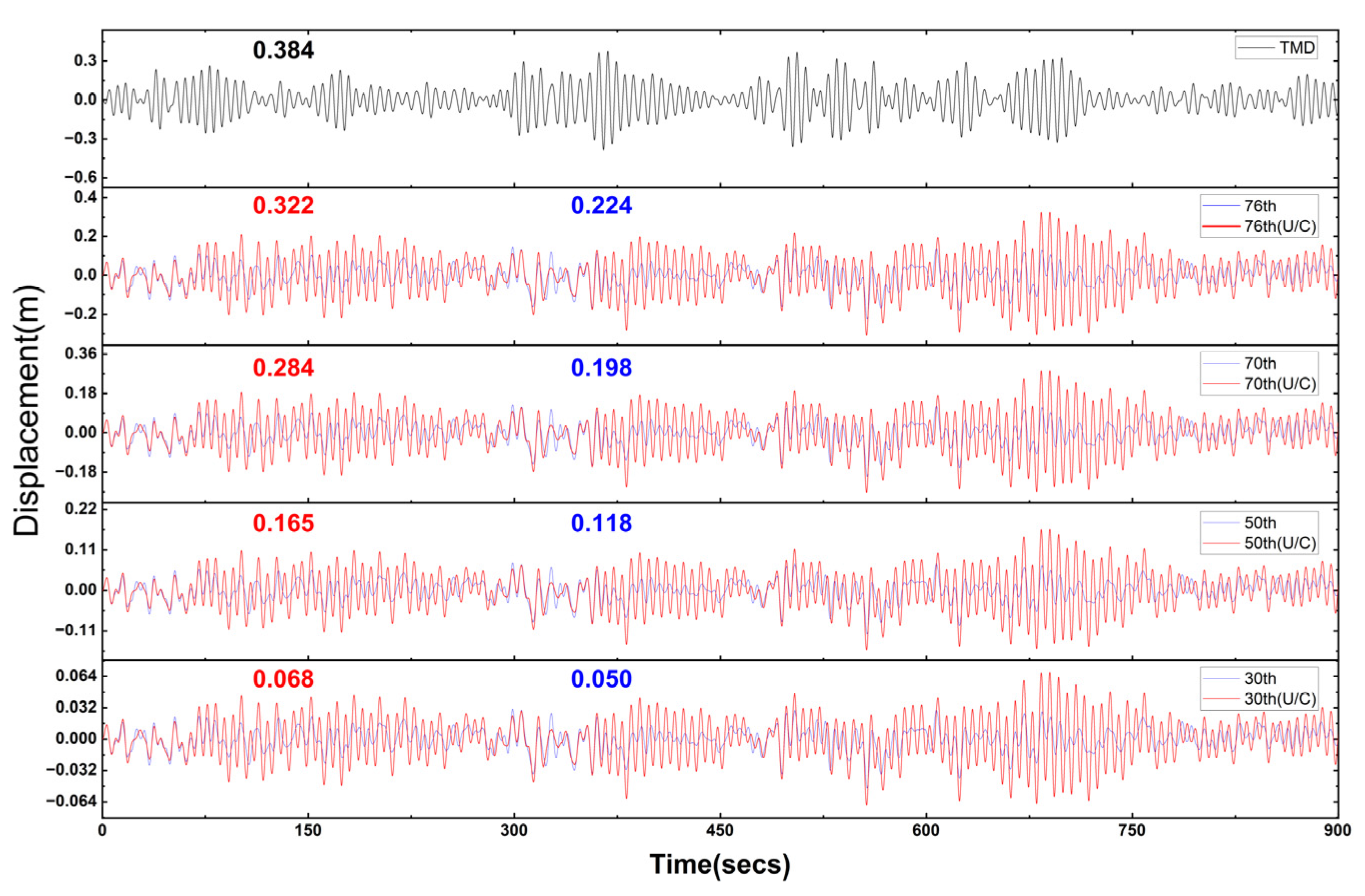
Figure 7.
Acceleration Response Time History for R₁ at Various Floor Levels.
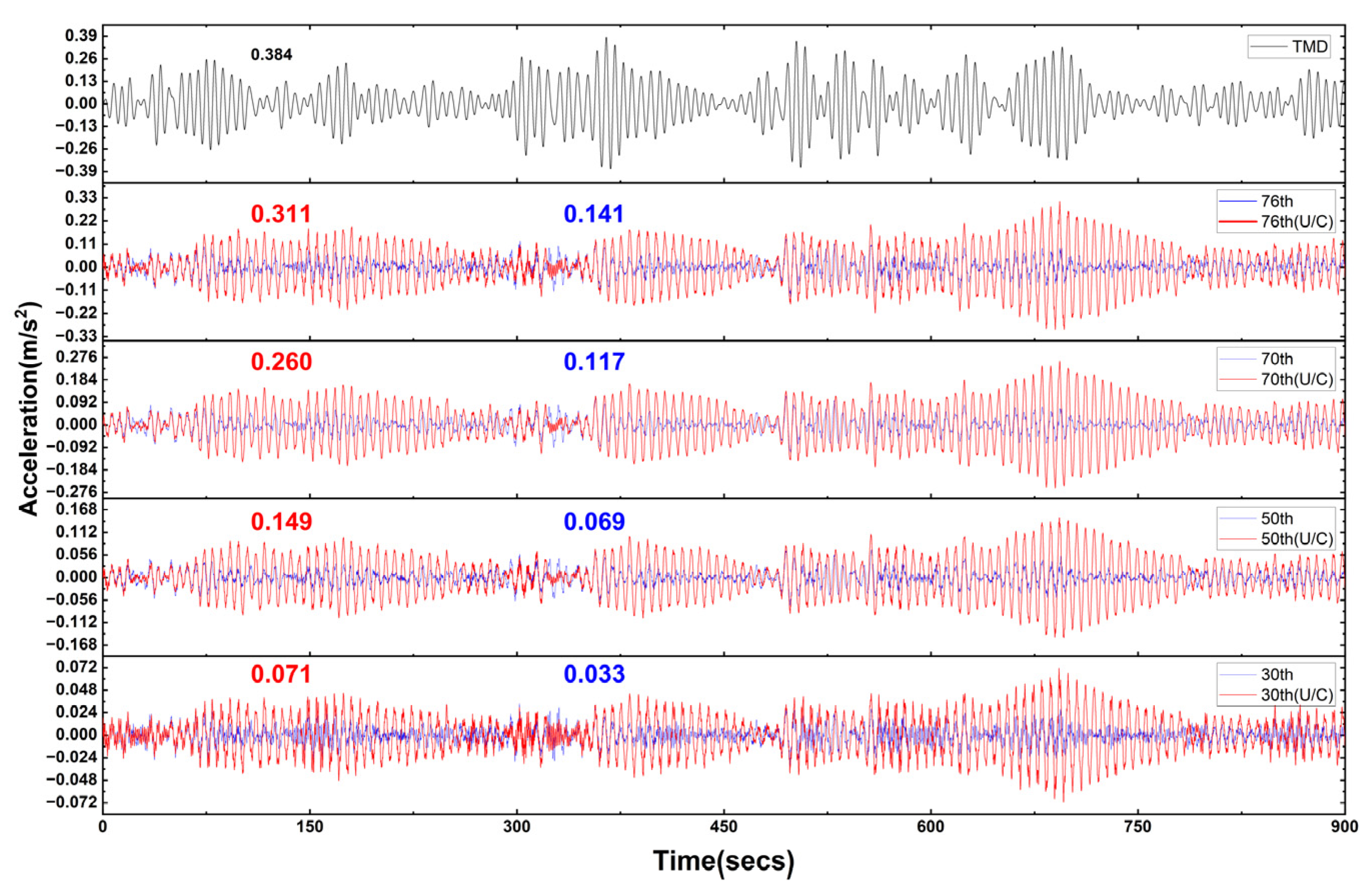
Figure 8.
RMS Floor Response under ±10% Uncertainty in Building Stiffness: (a) RMS Displacement with ΔK= +10%; (b) RMS Acceleration with ΔK= +10%; (c) RMS Displacement with ΔK= −10%; (d) RMS Acceleration with ΔK= −10%.
Figure 8.
RMS Floor Response under ±10% Uncertainty in Building Stiffness: (a) RMS Displacement with ΔK= +10%; (b) RMS Acceleration with ΔK= +10%; (c) RMS Displacement with ΔK= −10%; (d) RMS Acceleration with ΔK= −10%.
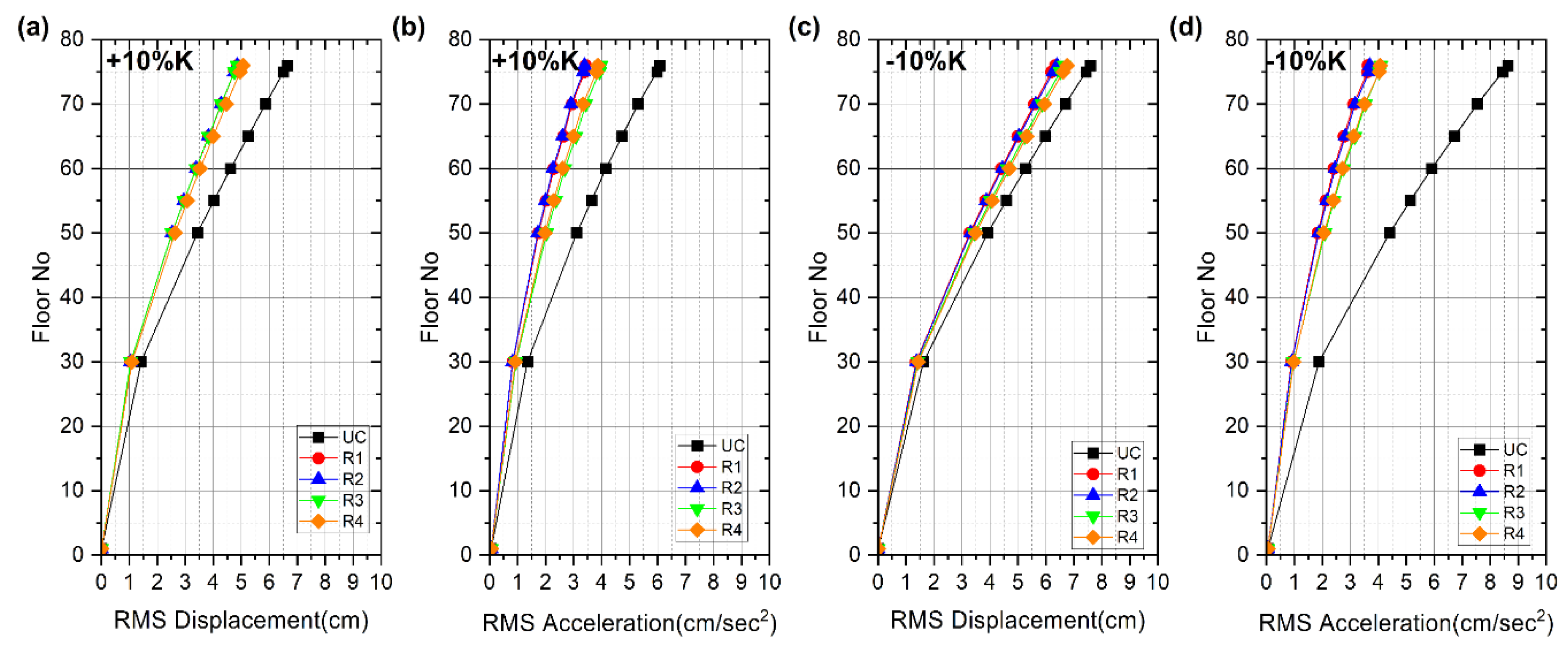
Figure 9.
Peak Floor Response under ±10% Uncertainty in Building Stiffness: (a) Peak Displacement with ΔK= +10%; (b) Peak Acceleration with ΔK= +10%; (c) Peak Displacement with ΔK=−10%; (d) Peak Acceleration with ΔK= −10%.
Figure 9.
Peak Floor Response under ±10% Uncertainty in Building Stiffness: (a) Peak Displacement with ΔK= +10%; (b) Peak Acceleration with ΔK= +10%; (c) Peak Displacement with ΔK=−10%; (d) Peak Acceleration with ΔK= −10%.
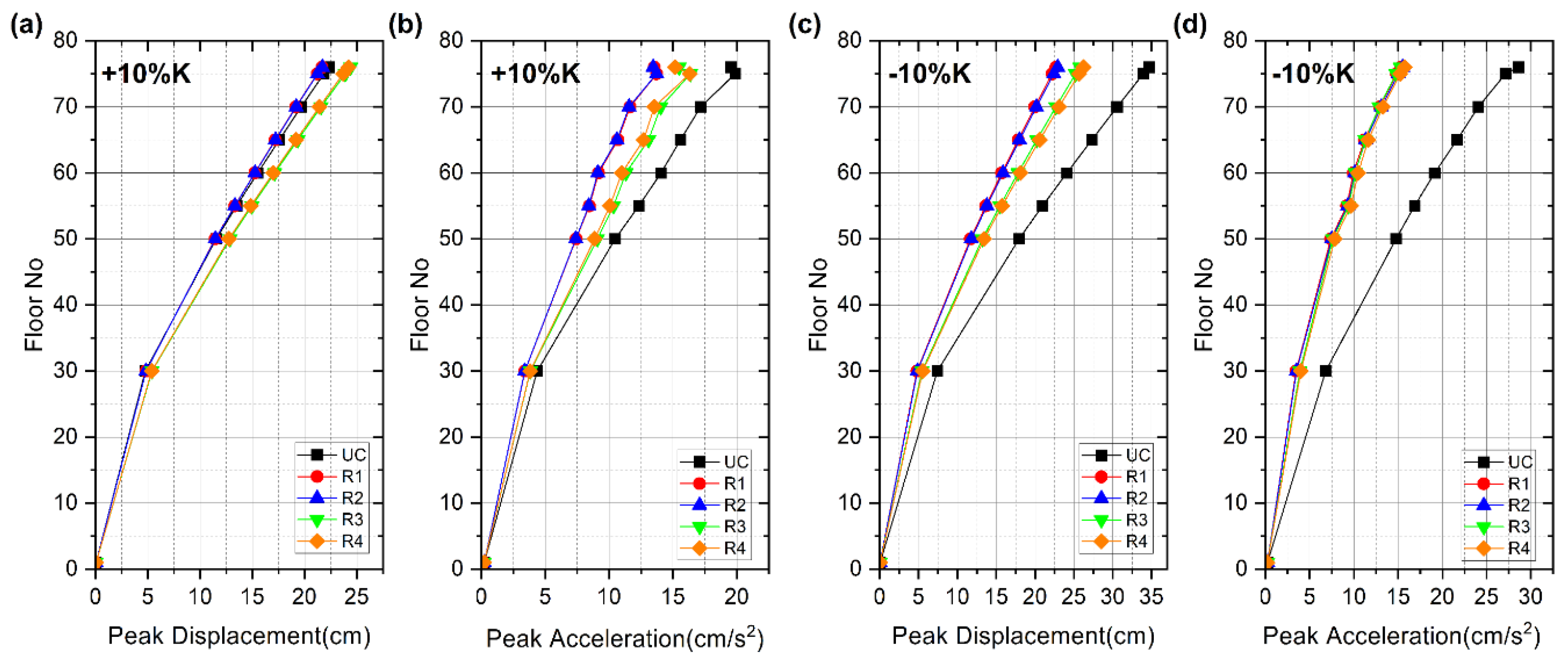
Figure 12.
Top floor response with 1% mass ratio with +10% stiffness uncertainty : (a) Displacement response; (b) Acceleration response.
Figure 12.
Top floor response with 1% mass ratio with +10% stiffness uncertainty : (a) Displacement response; (b) Acceleration response.
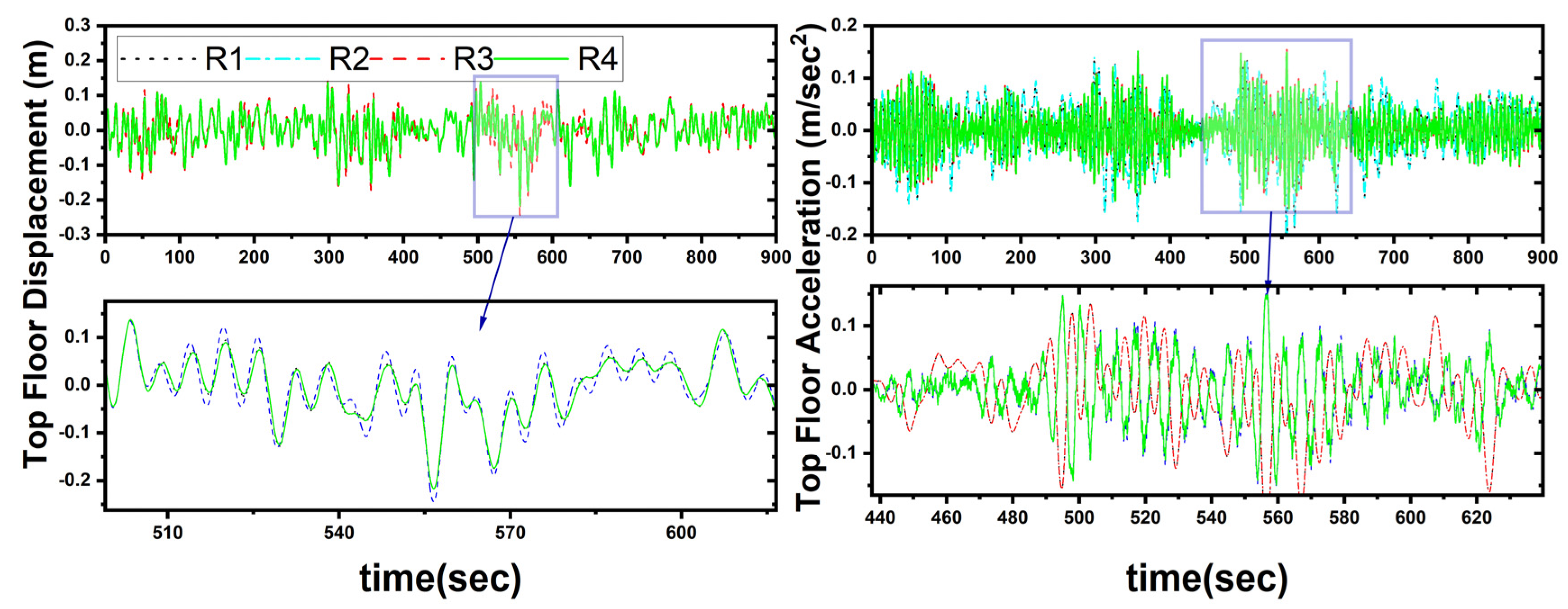

Table 1.
Performance Quantities for Control Strategies R₁ to R₄.
| Roots | RMS response | Peak response | ||||||||||
| 0.533 | 0.359 | 0.537 | 0.428 | 0.533 | 0.359 | 0.696 | 0.453 | 0.712 | 0.518 | 0.696 | 0.453 | |
| 0.536 | 0.361 | 0.540 | 0.430 | 0.536 | 0.361 | 0.710 | 0.457 | 0.726 | 0.521 | 0.710 | 0.457 | |
| 0.550 | 0.391 | 0.553 | 0.457 | 0.550 | 0.391 | 0.744 | 0.483 | 0.759 | 0.555 | 0.744 | 0.483 | |
| 0.555 | 0.395 | 0.558 | 0.461 | 0.555 | 0.395 | 0.773 | 0.488 | 0.788 | 0.565 | 0.773 | 0.488 | |
Table 2.
RMS response quantities: Displacement (cm) and Acceleration (cm/s2)
| Opt. Para. | Un-cont. | |||||||||
| – | 0.01 | 0.01 | 0.01 | 0.01 | ||||||
| – | 0.9852 | 0.9950 | 0.9852 | 0.9950 | ||||||
| – | 0.0998 | 0.1001 | 0.0502 | 0.0502 | ||||||
| Floor No. | ||||||||||
| 1 | 0.02 | 0.06 | 0.01 | 0.06 | 0.01 | 0.06 | 0.01 | 0.06 | 0.01 | 0.06 |
| 30 | 2.15 | 2.02 | 1.17 | 0.82 | 1.17 | 0.83 | 1.20 | 0.88 | 1.21 | 0.89 |
| 50 | 5.22 | 4.78 | 2.81 | 1.70 | 2.82 | 1.71 | 2.89 | 1.86 | 2.92 | 1.88 |
| 55 | 6.11 | 5.59 | 3.28 | 1.97 | 3.29 | 1.98 | 3.38 | 2.16 | 3.41 | 2.18 |
| 60 | 7.02 | 6.42 | 3.77 | 2.23 | 3.78 | 2.24 | 3.88 | 2.44 | 3.91 | 2.47 |
| 65 | 7.97 | 7.31 | 4.26 | 2.57 | 4.28 | 2.58 | 4.39 | 2.81 | 4.43 | 2.84 |
| 70 | 8.92 | 8.18 | 4.77 | 2.87 | 4.79 | 2.89 | 4.92 | 3.14 | 4.96 | 3.18 |
| 75 | 9.92 | 9.14 | 5.29 | 3.33 | 5.32 | 3.35 | 5.46 | 3.62 | 5.51 | 3.66 |
| 76 | 10.14 | 9.35 | 5.41 | 3.36 | 5.43 | 3.38 | 5.58 | 3.66 | 5.63 | 3.69 |
| TMD | – | – | 11.44 | 11.43 | 11.37 | 11.59 | 15.59 | 15.37 | 15.61 | 15.69 |
Table 3.
Peak response quantities: Displacement (cm) and Acceleration (cm/s2).
| Opt. Para. | Un-cont. | |||||||||
| – | 0.01 | 0.01 | 0.01 | 0.01 | ||||||
| – | 0.9852 | 0.9950 | 0.9852 | 0.9950 | ||||||
| – | 0.0998 | 0.1001 | 0.0502 | 0.0502 | ||||||
| Floor No. | ||||||||||
| 1 | 0.05 | 0.22 | 0.04 | 0.21 | 0.04 | 0.21 | 0.04 | 0.21 | 0.04 | 0.21 |
| 30 | 6.84 | 7.14 | 5.01 | 3.39 | 5.10 | 3.36 | 5.32 | 3.57 | 5.52 | 3.50 |
| 50 | 16.59 | 14.96 | 11.88 | 6.93 | 12.10 | 7.06 | 12.65 | 7.80 | 13.13 | 8.28 |
| 55 | 19.41 | 17.48 | 13.82 | 8.46 | 14.08 | 8.53 | 14.73 | 9.30 | 15.29 | 9.75 |
| 60 | 22.34 | 19.95 | 15.81 | 9.18 | 16.11 | 9.26 | 16.86 | 10.12 | 17.51 | 10.34 |
| 65 | 25.35 | 22.58 | 17.83 | 10.55 | 18.19 | 10.65 | 19.04 | 11.57 | 19.78 | 11.75 |
| 70 | 28.41 | 26.04 | 19.88 | 11.77 | 20.28 | 11.90 | 21.25 | 12.85 | 22.07 | 13.04 |
| 75 | 31.59 | 30.33 | 22.00 | 13.30 | 22.44 | 13.45 | 23.53 | 14.48 | 24.44 | 14.70 |
| 76 | 32.30 | 31.17 | 22.48 | 14.12 | 22.93 | 14.24 | 24.04 | 15.07 | 24.98 | 15.22 |
| TMD | – | – | 38.44 | 38.40 | 38.35 | 39.08 | 53.78 | 53.00 | 55.29 | 55.58 |
Table 4.
Effect of ±10% Stiffness Uncertainty on Structural Performance Parameters.
| Root | Stiffness Uncertainty |
RMS response | Peak response | ||||||||||
| ΔK = +10% | 0.730 | 0.565 | 0.734 | 0.613 | 0.730 | 0.565 | 0.971 | 0.692 | 0.991 | 0.729 | 0.971 | 0.701 | |
| ΔK =-10% | 0.603 | 0.421 | 0.606 | 0.485 | 0.603 | 0.421 | 0.654 | 0.534 | 0.652 | 0.579 | 0.654 | 0.534 | |
| ΔK = +10% | 0.729 | 0.558 | 0.733 | 0.607 | 0.729 | 0.558 | 0.972 | 0.688 | 0.992 | 0.727 | 0.972 | 0.702 | |
| ΔK =-10% | 0.609 | 0.428 | 0.611 | 0.491 | 0.609 | 0.428 | 0.661 | 0.542 | 0.659 | 0.586 | 0.661 | 0.542 | |
| ΔK = +10% | 0.767 | 0.654 | 0.771 | 0.694 | 0.767 | 0.654 | 1.093 | 0.791 | 1.113 | 0.849 | 1.093 | 0.837 | |
| ΔK =-10% | 0.468 | 0.474 | 0.472 | 0.533 | 0.468 | 0.474 | 0.743 | 0.533 | 0.739 | 0.590 | 0.743 | 0.533 | |
| ΔK = +10% | 0.761 | 0.636 | 0.765 | 0.678 | 0.761 | 0.636 | 1.084 | 0.775 | 1.105 | 0.833 | 1.084 | 0.834 | |
| ΔK =-10% | 0.643 | 0.472 | 0.645 | 0.530 | 0.643 | 0.472 | 0.756 | 0.550 | 0.752 | 0.605 | 0.756 | 0.550 | |
Disclaimer/Publisher’s Note: The statements, opinions and data contained in all publications are solely those of the individual author(s) and contributor(s) and not of MDPI and/or the editor(s). MDPI and/or the editor(s) disclaim responsibility for any injury to people or property resulting from any ideas, methods, instructions or products referred to in the content. |
© 2025 by the authors. Licensee MDPI, Basel, Switzerland. This article is an open access article distributed under the terms and conditions of the Creative Commons Attribution (CC BY) license (http://creativecommons.org/licenses/by/4.0/).
Copyright: This open access article is published under a Creative Commons CC BY 4.0 license, which permit the free download, distribution, and reuse, provided that the author and preprint are cited in any reuse.


