
Submitted:
09 July 2025
Posted:
11 July 2025
You are already at the latest version
Abstract
In this paper we propose a crossover operator for genetic algorithms with binary chromosomes population based on the cellular automata (CGACell). After presenting the fundamental elements regarding cellular automata with specific examples for one- and two- dimensional cases, the the most widely used crossover operators in applications with genetic algorithms are described and the crossover operator based on cellular automata is defined. Specific forms of the crossover operator based on the ECA and 2D CA cases are described and exemplified. The CGACell crossover operator is used in the genetic structure to improved the KNN algorithm in terms of the parameter represented by the number of nearest neighbors selected by the data classification method. Validity and practical performance testing is performed on image data classification problems by optimizing the nearest-neighbors-based algorithm. The experimental study on the proposed crossover operator, by comparing the algorithm based on CGACell with standard data classification algorithms such as PCA, Kmeans or KNN, attests good qualitative performance in terms of correctness percentages in the recognition of new images, in classification applications of facial image classes corresponding to several persons.
Keywords:
genetic algorithms (GA)
; cellular automata (CA)
; elementary cellular automata (ECA)
; crossover operators
; K-nearest neighbors (KNN)
; kmeans
; face images classification
; principal component analysis (PCA)
1. Introduction
The numerous theoretical and practical applications, conferred by the ability to offer innovative solutions for a varied range of complex problems, have positioned optimization techniques in the attention of researchers from various fields such as machine learning, operations research, computational systems biology, mechanics or economics and finance. Among the categories of optimization techniques, we can specify stochastic optimization, linear programming, quadratic programming, continuous optimization, discrete optimization, unconstrained optimization, as well as evolutionary algorithms that are able to find solutions in complex and large data spaces [4,19,33]. The main evolutionary algorithms used are: Genetic Algorithms, Particle Swarm Optimisations (PSO), Ant Colony (AC), Simulated Annealing (SA), Immune Algorithms (IA), Artificial Bee Colony (ABC), Firefly Algorithm (FA) and Differential Evolution (DE). Realizing the percentages of use in applications, with a value of over 50%, genetic algorithms were chosen [49]. Among the various applications of genetic algorithms, the most important is the optimization of problems by determining the optimal solutions. Genetic algorithms are optimization algorithms inspired by the process of natural selection through which representative individuals are advantaged and were developed by Goldberg (1989) [19]. Applications using GA include: data clustering and mining, neural networks, image processing, feature selection for machine learning, medical science, learning robot behavior, traveling salesman problem, vehicle routing problem, financial markets, manufacturing system or mechanical engineering design [25,37].
In the process of searching for solutions in the solution space, a genetic algorithm performs an evolutionary transformation of the population, over several generations, by using the genetic operators of selection, crossover and mutation, and the quality of the descendants of the chromosomes in the current population is evaluated by the function fitness that decides the composition of the new population of chromosomes. An essential role in the evolutionary process of a genetic algorithm is represented by the reproduction stage in which the chromosomes, selected to participate in the formation of the new generation, determine the new descendants through the gene crossing operation [25,39,51]. Thus, the crossover problem has many developments in specialized research, establishing experimental performances from classic methods (with one point, with two or more crossing points, uniform or order) to techniques to solve object classification problems (Looseness control crossover or Greedy partition crossover) [5,30,31,46,48].
The aim of the paper is to propose a crossover operator for genetic algorithms using cellular automata and to establish the experimental performance in specific data classification applications.
2. The Cellular Automata
Cellular automata are among the oldest models of natural computing, the first studies being carried out by John von Neumann in the 1940s. Cellular automata have a biological motivation rendered by the design of artificial systems that have the property of self-replication, having as inspiration the model from the level of the human brain in which memory and processing units do not operate separately but are able to work together [26]. At the S. Ulam’s suggestions, J. Neumann developed the system by considering a discrete space consisting of a two-dimensional mesh of machines with finite states. Given the ability to solve problems of high complexity, cellular automata have been used in the fields of natural sciences, mathematics or computer science [43,52]. After A. Burks published J. von Neumann’s book in 1966, more scientists became interested in cellular automata. John Conway in 1970 introduced a CA called Game of Life. He used a two-dimensional lattice with two possible states for the cells (dead and alive) and the transition being made based on the neighboring cells of the dead or alive type [17]. A cellular system constitutes a basic framework or cellular space in which the events of the automaton can take place and the simple and precise rules applied will ensure the functioning of the system [6]. The cellular space is defined by an n-dimensional space together with a neighborhood relation defined on this space. The neighborhood relation associates each cell in the cell space with a lot of neighboring cells. A cellular automata is specified by a finite list of states for each cell, an initial state and a transition function that, based on the neighborhood relationship at time t, establishes a new state at time corresponding to each cell. In the standard formulation, CA can be studied in the () space and using an alphabet L. In recent years, several generalizations relative to the CA alphabet have been developed through the use of groups, vector spaces or commutative monoids [8,9,10,54]. For the case of a group V and an alphabet set L, the specific elements (configuration space, shift action, memory set and local function) for defining a cellular automaton are given below [7,27].
Definition 1 (configuration space)The configuration space represents the set of functions defined on V with values in L of the form .
Definition 2 (shift action)The shift action of V on is defined by , for all , .
Definition 3 (memory set and local function)The memory set represents a subset M of the set V () and a local function is defined by a function .
Definition 4 (cellular automaton)A cellular automaton is defined by a function that satisfies the property , with memory set M and local function φ, , and where denotes the restriction to M of a configuration in .
(ECA) 1D CA).Remark 1 (Elementary Cellular Automaton The elementary cellular automaton represents a one-dimensional cellular automaton (1D CA) with two states (), and the transition rule in a new state of a cell depends only on the neighborhood formed with the adjacent cells (the current cell and the left and right neighbors of the cell).
An ECA capable of universal computation due to the property of simulating any Turing machine, and thus the system is able to recognize or decide other sets of data manipulation rules, is a one-dimensional CA corresponding to rule 110 of the Wolfram Code, establishing the resulting states for the eight possible configurations associated for a cell with its two adjacent neighbors.
To establish the particular case of the ECA, the settings corresponding to the one-dimensional case with two cell states are considered by: and . With these conditions, the configuration space , , where , , and represents the value of the image of i by the function , . In this case the shift action of on can be written by the following relation .
Also, the memory set M is established based on the pattern associated with the neighborhood used for the cells of the automaton by and the local function of the automaton is defined by ().
The cellular automaton is defined based on set memory M and the local function φ through the function that satisfies the property , , and where denotes the restriction to of a configuration in .
Using the Wolfram code and choosing rule 110 and rule 90 for the local function φ, the ECA can be written according to the values specified in Table 1 (ECA110) and Table 2 (ECA90) respectively, in which both the state values of the neighboring cells and the output values associated by rule 110 and rule 90 (with binary representation and ) are shown. The results of ECA 110 for generations of evolution of cell states of a cellular automaton with cells are shown in Table 3. The results of ECA 90 for generations of evolution of cell states of a cellular automaton with cells are shown in Table 4.
Table 5 shows the binary images associated with the state values of the elementary automata cells corresponding to rules 30, 90, 99, 110, respectively, 158 (denoted by E 30, E 90, E 99, E 110, respectively, E 158) after 150 of cell evolution and by using 31 in the initial sequence.
(2D CA)).Remark 2 (Two-dimensional cellular automata There are several approaches in the field to define two-dimensional cellular automata (2D CA). As in the case of ECA, the components of a cellular automaton are the lattice (set of cells - each one in a state), the neighborhood and the local transition rules. The rules represent the communication between each cell and its neighborhood, it is local, uniform for the whole lattice and synchronous. The rules determine the global evolution of the system at each discrete step in time. The lattice represents the V group also considered for the definition of one-dimensional cellular automata ECA. If was considered for ECA, is considered for the definition of two-dimensional cellular automata. The neighborhood is the set of cells taken into account in the evolution of the cell. The most used are the Von Neumann and Moore neighborhoods [35]. The von Neuman neighborhood model is a template that contains the immediate north, south, east, and west neighbors of the current cell. The Moore neighborhood model is a template that includes all the immediate neighbors of the current cell (from the north, south, east, west, northeast, northwest, southeast and southwest). Over time, several models with adequate results in applications have been added to these templates [13,50] (Figure 1). The states of a 2D CA at any moment can be represented by a binary matrix A of size , that will contain the cells of the automaton. According to the definition in [35], for the von Neumann neighborhood consisting of five neighbors and the lattice A, the state of a cell in position () of A, is updated from a new generation () through a relation of the form: with , , , where is the number of generations of evolution of the automaton. Given the size of the considered neighborhood with neighbors, we have possible states associated with cells in the neighborhood based on a rule for associating bits from the binary representation of numerical values in the interval .
Another variant used is the one in which the state of the current cell is determined by a rule based on a function f with the argument represented by the sum of the values of the states of the neighbors retrieved according to the template used with , and with the extension of through by using only the four neighbors. In this case the sum of the binary state of the neighbors are maximally 4 and we may establish that the new state of the cell to be equal with the bit value by position from the binary representation for the choose rule in numerical domain like . By using the variant based on the function, the images associated with the evolution generations of 2D CA in Figure 2, Figure 3, Figure 4, Figure 5, Figure 6 and Figure 7 are generated. The two-dimensional space of the cellular automaton is initialized by using a square matrix of size 28, with all state values equal to 0, with the exception of the cell located in the middle of the matrix, which is initialized with the value 1, for all cases represented graphically. Figure 3 and Figure 4 are shown in two dimensions results of the cellular automaton for the von Neumann neighborhood case and the application of the function for rules 6 (line 1), 9 (line 2), 17 (line 3), 21 (line 4), and 26 (line 5), respectively. In Figure 3 are displayed the images corresponding to the results of the automaton along the first 10 generations of evolution and in Figure 4 are displayed the images associated with the automaton for generations from 5 to 50 but displayed with the progression rate equal to 5. Figure 6 and Figure 7 are shown in two dimensions results of the cellular automaton for the Moore neighborhood case and the application of the function for rules 33 (line 1), 90 (line 2), 94 (line 3), 150 (line 4), 234 (line 5), 261 (line 6), 322 (line 7), 330 (line 8), 386 (line 9) and 490 (line 10), respectively. In Figure 6 are displayed the images corresponding to the results of the 2D CA along the first 10 generations of evolution and in Figure 7 are displayed the images associated with the 2D CA for generations from 5 to 50 but displayed with the progression rate equal to 5. The graphic representation of the evolution of a 2D CA along 100 generations of cellular evolution is made in Figure 2 and Figure 5 in which the images obtained by using a von Neumann neighborhood with rule 9 are shown, respectively of a Moore neighborhood with rule 330.
3. Genetic Algorithms
3.1. The General Presentation of GA
Genetic algorithms are adaptive heuristic search techniques based on principles genetics and natural selection, stated by Darwin (survival of the best adapted). The mechanism is similar to the biological process of evolution. According to this process only the species that adapt better to the environment are able to survive and evolve over generations, while those less adapted do not manage to survive and eventually disappear, as a result of natural selection. As practical applications, genetic algorithms are most often used in solving problems of optimization, planning or search [25,35].
The fitness function is used to measure the quality of the chromosomes and is formulated starting from the numerical function to be optimized. The fitness function has a key role at the level of the genetic algorithm through the ranking of chromosomes and the decisions it can produce in the choice of offspring throughout the calculation generations.
The genetic operators used by genetic algorithms are:
- Selection: is an important stage of a genetic algorithm in that it determines the way of choosing the parent chromosomes that will participate in the recombination stage and produce new individuals in the current population. Among the most important selection techniques are are roulette wheel, rank, tournament, boltzmann and stochastic universal sampling [16,24].
- Crossover: determines the transformation method of the genes from the parent chromosomes to result in new candidate chromosomes for the next generation.
- The mutation: based on some probability values, certain values of the genes of a descendant chromosome can be changed. Mutation is an operator that maintains the genetic diversity from one population to the next population.
For the stages of selection, recombination and mutation, there are several application and calculation methods used in the field of genetic algorithms. Depending on the specifics of the application and the way chromosome genes are represented, certain methods associated with the application of genetic operators are chosen, in order to obtain good results in experimental studies [19,25,40,51]. The initialization stage at the level of the genetic algorithm is represented by the evaluation of the format of the input data corresponding to the domain of the problem being optimized and the encoding of the input data, as a rule, by binary values or real values. The initial population will consist of a lot of input vectors with binary or real values as chromosomes. Genetic operators will be applied to the population of chromosomes over several generations of evolution, until the stopping condition is fulfilled, by forming new generations based on the fitness function that evaluates the quality of the individuals in the current population.
The general structure of a genetic algorithm (also shown in the Figure 8)
- Set the time .
- Creation of the initial population .
- Evaluation of the initial population with the fitness function .
-
While the final condition is false:
- .
- Selection of new generation from .
- Application of the crossover operator for the selected chromosomes for the new population .
- Evaluation of the new population with the fitness function and determining the final chromosomes (keeping the best chromosomes or according to a certain rule for the formation of new generations).
3.2. Crossover Methods Used by GA
Crossover operators are used to generate offspring chromosomes by recombining selected individuals from the current population to form the new generation. Among the most used crossover operators are single point, two-point, k-point, uniform, partially matched, order, precedence preserving crossover, shuffle, reduced surrogate and cycle [25,30].
Single-point crossing determines the offspring by taking the values of the genes from one parent up to the crossing point and the genes from the other parent after the crossing point position [48]. Application examples for one-point crossover is in Figure 9 where the gene values are binary values and in Figure 10 where the gene values are real values.
In a two-point and k-point crossing, two or more random crossing points are selected, and the offspring are obtained by taking the genetic information from each parent by swiping in the crossing points [48]. Application examples for k-point crossover (, ) is in Figure 11 where the gene values are binary values and in Figure 12 where the gene values are real values. Uniform crossover is achieved by taking genes from the first or second parent evenly based on a uniform random parameter, for each gene, that decides which parent the gene is taken from [48]. Application examples for uniform crossover (the uniform parameter establishes the modification of the genes on positions 4 and 7) is in Figure 13 where the gene values are binary values and in Figure 14 where the gene values are real values. Partially-Mapped Crossover (PMX) was proposed by D. Goldberg and R. Lingle and is one of the most used operators in genetic algorithm applications [20]. The working method for this operator includes several stages: two parents are selected for recombination, the values of the two cutting positions are determined that determine the mapping of the values from one parent to the other, the analysis of the mapping rules and their application to the gene areas of outside the mapping area at the level of the two parents. In the end, two descendants are obtained that in the cutting area keep the genes of one of the parents, and outside the cutting area certain values are updated based on the mapping between the two parents. An example regarding the steps mentioned for the PMX crossover is shown in Figure 15 by considering the cut positions equal to 3 and 6 for two parent chromosomes with 9 genes. Order crossover (OX) is another crossover method that is based on the establishment of cut-off points that induce the preservation of the values of the genes from one parent in the respective intervals, and the rest of the genes are completed with the values from the other parent from which the values taken are excluded already from the first parent [36]. An example for OX crossover is shown in Figure 16 having cut positions equal to 2, 4, 6 and 7 for two parent chromosomes with 9 genes in the component.
In addition to the previously exemplified crossing methods in this section, many other crossover techniques have been developed by making changes to the basic ones or based on other working principles. Thus, we can specify: Average Crossover (AX), Shuflle Crossover, Modified Order Crossover (MOC), Modified Partially-Mapped Crossover (MPMX), Cycle Crossover (CX), Voting Recombination Crossover operator (VR), Masked crossover (MkX), Heuristic crossover (HX), Edge Recombination crossover (ER), Alternate Edges Crossover, Greedy Subtour Crossover [5,30,32,33,37,39]. A series of crossover techniques used to solve object classification problems are added, such as: Looseness control crossover (LCC) and Headless chicken crossover (HCC) for classification problems, Product Geometric Crossover (PMX) for Sudoku, Simplex crossover, Multi-Parent Crossover, Multi-Parent feature Crossover (MFX), Multicut crossover (MX) and Seed crossover (SX), Conflict elimination crossover (CEX) and Greedy partition crossover (GPX) for Graph coloring problem and others [31,34,42,44,45,46,48,56].
4. CGACell Operator for Binary Chromosomes Population of Genetic Algorithms
In this section, the crossover operator based on cellular automata is introduced () for the case of chromosomes represented by genes with binary values.
Consider a cellular automaton and a genetic algorithm G with the population consisting of genes with binary values , where is the i chromosome, , for and , is the number of chromosomes in at time and is the number of genes of the chromosomes with .
Definition 5
(CGACell Crossover operator). The crossover operator is defined for a population of binary chromosomes , a cellular automaton γ (k- dimensional, ) and a neighborhood established according to a given template for taking neighbors, , , , is the elements number of , as follows:
where represents the descendant chromosome obtained by applying a k-dimensional cellular automaton () on a set of chromosomes (with ) chosen by the selection techniques established by GA, with a cardinality correlated with the size of the neighborhood used .
Remark 3
(CGACell ECA). In the one-dimensional case of cellular automata, the crossover operator CGACell ECA is obtained. We have the relationship , where the neighborhood consists of 3 elements represented by the neighboring cells on the left and right of the current cells, , , , , is the elements number of .
Observation The CGACell ECA operator can be applied in two ways: individually on each chromosome chosen in the selection stage for recombination, or mixed on genes on the same positions (or corresponding through a mapping) from a number of chromosomes chosen for recombination equal to the cardinality of the set of memory M of the cellular automaton (equal to three for the exemplified case).
Example 1 - CGACell ECA
The method of applying the operator CGACell ECA at the chromosome level using an ECA with 110 previously presented in section CA ( 1) is illustrated in Figure 17. Also, the results of the CGACell ECA crossover operator for 90 are illustrated in Figure 18. The two offspring chromosomes correspond to the chromosomes chosen by selection to participate in reproduction for GA. Cells that change their state by applying CGACell ECA Crossover and according to 110 or 90 are highlighted on a white colored background for each descendant. For cells in extreme positions, they are generically filled with inactive values equal to zero for full ECA rule application.
Example 2 - CGACell ECA
The crossover operator CGACell ECA can also be applied in mixed mode on three chromosomes, chosen after the selection stage. Let the set of chromosomes chosen for reproduction in the GA selection stage be of the form from the current population .
Having the representation of chromosomes , for () and , , the neighborhood is formed for the application of the CGACell ECA crossover operator, by , with , , , , .
The application of the operator CGACell ECA at a mixed level on three chromosomes using ECA with 110 is presented in Figure 19 and by using ECA with 90 in Figure 20. We can see the descendant chromosome ( or ) obtained by CGACell ECA crossover using 110 or 90 with the neighborhood formed by taking the values of the genes on the same positions from the three chromosomes selected for crossing.
Descendant chromosome ( or ) cells that differ from the corresponding states in chromosome two, after applying CGACell ECA Crossover and 110 or 90, are highlighted on a white background.
Remark 4 (CGACell 2D CA)
By using two-dimensional cellular automata, the version of the CGACell 2D CA crossover operator is obtained. We have the relationship , where the neighborhood is built in accordance with the templates presented for two-dimensional cellular automata (remark 2, Figure 1), the most representative being the von Neumann neighborhood with five neighbors, respectively, the Moore neighborhood with nine neighbors, , , and is the number of neighbors in .
Property 1.
The configuration space of the cellular automaton V is formed by completing the two-dimensional space with chromosomes chosen from the current population to participate in the creation of descendants and the new generation of individuals.
Example 3 - CGACell 2D CA
The results of applying the 2D CA crossover operator are displayed graphically in Figure 21, Figure 22, Figure 23 and Figure 24. Are graphical representations of the binary images corresponding to the application of CGACell 2D CA crossover with evolution in 100 generations of the chromosomes selected in to denote the two-dimensional configuration space of the 2D CA automaton are presented, for von Neumann neighborhoods with rules 6 and 11, respectively, Moore with rules 330 and 490 with the use of 10 chromosomes consisting of 20 genes. In all four figures, the chromosomes descended from time t () are displayed by binary images of size 10 (the number of chromosomes selected for recombination) multiplied by 20 (the number of genes of each chromosome in the population) and are obtained by applying CGACell 2D CA on the parent chromosomes shown in the previous evolution generation .
Remark 5 (Application in data classification with KNN method of theCGACellcrossover-based genetic algorithm)It is considered a data classification application using the KNN algorithm based on the nearest neighbors [2,3,22]. Performance testing in data classification through the KNN algorithm is performed on the basis of a set of training data and a set of test data , both sets of data from multiple data classes, and the key element that determines the improvement of the results is the parameter k number of neighbors taken into account for classification. For the optimal establishment regarding the performance in classification of the value of the k parameter, it can be achieved by applying a genetic algorithm based on CGACell crossover. The genetic algorithm based on the CGACell crossover operator (usually the ECA or 2D CA versions are used), denoted by CGACell-GA for data classification by the nearest neighbors method includes the following work steps:
- +
- The population is made up of chromosomes with binary values corresponding to the binary representation of the values in the field of representation of the k parameter that designates the number of nearest neighbors that will decide, depending on the classes of origin, the classification results for the KNN algorithm.
- +
- The population consists of binary chromosomes with a size equal to the number of bits in the representation of the maximum value () in the range of possible values for the parameter k. Let be the maximum value of k established based on the number of data used for training by , , where is the number of the training data input from class i, ), is number of data classes, and is the selection weight for the maximum number of neighbors with values, usually chosen, in the interval and .
- +
- The population of the genetic algorithm consists of chromosomes as follows: , where is the i chromosome, , , for and , with is the number of chromosomes and in the experiments a value adapted to the total number of training data was used.
- +
- The fitness function , is represented by the performance (percentage of correct classification) in the classification of the test data obtained by using a number of nearest neighbors equal to the value in base ten of the chromosome argument of the function.
- +
- The selection is carried out by the roulette type method after determining the scaling function for the chromosomes in the current population (the moment of time ), establishing the selection probabilities and the actual selection of chromosomes with and is the number of selected chromosomes for the crossing stage based on randomly generated values in the numerical range .
- +
- The CGACell crossover is performed for the chromosomes selected from the set through several transformation methods at the level of the binary vectors from the chromosome representations. CGACell ECA or 2D CA crossover are used. For each crossing case, the corresponding experimental results were established in the classification of the test data from the test set .
- +
- The mutation is carried out at the level of the chromosomes in the set resulting after the step of crossing the binary genes. The mutation operation involves updating certain genes, in a very small proportion (between ) by transforming the chosen genes into the complementary binary value.
- +
- After the genetic mutation operation, the set of chromosomes in is reevaluated by applying the fitness function in order to establish their quality and the new generation of chromosomes is formed by choosing the best chromosomes.
- +
- The algorithm is repeated by applying the genetic operators of selection, CGACell crossover and mutation and forming new generations with the best performing chromosomes until a predetermined maximum number of training generations is reached or the optimal value is reached or in the situation where the classification performance test data stagnates.
The experimental results regarding the application of CGACell crossover in KNN data classification showed good performance in a study compared to other classification methods and are presented in the experimental analysis section.
Related Work
In the specialized literature there are many optimization applications in which genetic algorithms are used with improvements at the crossover stage. E. Tafehi et al. introduced a new and improved method for GA based on Chaotic Cellular automata (CCA) along with influencing pseudo random number generator. The operations specific to the genetic algorithm of selection, mutation and crossover are influenced by pseudo random number generator and thus change the behavior of the evolution of chromosomes in the exploration space [41]. U. Cerruti et al. introduced an original implementation of a cellular automaton whose rules use a fitness function to select for each cell the best mate to reproduce and a crossover operator to determine the resulting offspring. They also created two generalizations of the game of life and other applications in the paper [11]. Deng et al. in the paper [14] proposed a hybrid cellular genetic algorithm with simulated annealing in which the genetic algorithm used together with cellular automata. They applied a hybrid cellular genetic algorithm combined with a simulated annealing algorithm to solve the TSP, and the experimental results showed the optimization performance of the hybrid cellular genetic algorithm. In the paper [29] M. Mitchell et al. have applied genetic algorithms to the design of cellular automata that can perform calculations that require global coordination. The proposed work method establishes for each chromosome in the population a candidate rule table. The evolution of CA with GA has provided an appropriate framework in which to study the mechanisms by which an evolutionary process could create complex coordinated behavior in decentralized distributed natural systems. S.J. Louis and G.L. Raines used a genetic algorithm to calibrate a cellular automaton that modeled mining activity on public land in Idaho and Western Montana. The genetic algorithm searches in the parameter space of the transition rules of a 2D CA to find the parameters of the rule that matches the observed mining activity data [28]. Also, with reference to the proposed application of the optimization of the KNN algorithm by using the proposed crossover operator, other results established in this direction can be mentioned. For example, the authors N. Suguna and K. Thanushkodi in the paper [38] presented an improved version of KNN where instead of considering all the training samples, the GA is employed to take k-neighbors straightaway and then calculate the distance to classify the test samples and before classification, initially the reduced feature set is received from a novel method based on Rough set theory hybrid with Bee Colony Optimization. In [23] the authors presented a novel approach for classifying heart disease by combines KNN with genetic algorithm. As a way to validate the proposed method, they tested with emphasis on heart disease and the experimental results showed that their algorithm enhance the accuracy in diagnosis of heart disease.
Experimental Analysis for CGACell Crossover Operator in Specific Tasks
The performance testing of the CGACell crossover operator based on cellular automata is performed in two-dimensional data classification applications (images). The CGACell crossover operator presented in this paper is used in image classification problems through the KNN algorithm to optimize the parameter k representing the number of nearest neighbors. The genetic algorithm (CGACell-GA) based on CGACell crossover is detailed in remark 5.
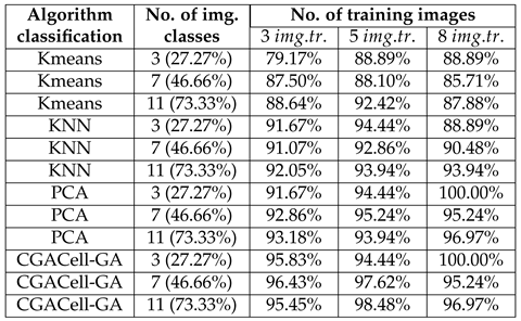
Experimental performances of the algorithm (CGACell-GA) are established for the problem of classifying classes of face images, corresponding to multiple individuals, from the free Yale Face database. The Yale database contains 165 images of faces corresponding to 15 people with 11 images each representing certain facial expressions or configurations (glasses, happy, left light, right light, sad, sleepy, surprised, wink, center light, no glasses and normal). The experimental results are achieved by the stability of the correctness percentages in the classification of image classes from the Yale image database. The performances in testing new images for the proposed algorithm are highlighted through an experimental comparative study with standard classification methods such as the KMeans algorithm, the Principal Component Analysis (PCA) algorithm and the standard KNN algorithm. In the comparative study, three cases are considered regarding the number of classes of images: the classification of 3 classes of images, the classification of 7 classes of images and, respectively, all the classes (11) of images available in the database. For each case of the number of classes of images, the correctness percentages in the classification of images corresponding to the use of three, five, and eight training images from each class of images are established. In all three cases, the number of images used for the training stage is represented by the labels Series1- three training images, Series2- five training images, and Series3- eight training images, in Figure 25, Figure 26, Figure 27 and Figure 28. Figure 28 shows results obtained from the experimental analysis based on the Yale image database for the classification of images from 3, 7 and 11 face image classes by using a name of 3, 5, respectively 8 training face images. Also, the numerical results obtained from the experimental analysis for the algorithm based on CGACell crossover, using the Yale image database for classifying images from face image classes 3, 7, and 11 and having successive values of 3, 5, and 8 training face images, respectively, and the rest of the images remained in the test set, are specified in Table 6.
Case I: For the first test, the images from three classes of images taken from the Yale face database are classified by applying the proposed CGACell-GA algorithm, as well as the KMeans, standard KNN and PCA algorithms. The percentages of correct classification of images from the three classes are graphically represented in Figure 25 for different values (three, five, and eight images, respectively) of the number of training images from each class of face images.
Case II: For the second test, the procedure is similar to the working method of case 1, except that seven classes of images are classified and the results are in Figure 26.
Case III: For the third test, the procedure is similar to the working method of cases 1 and 2, except that eleven classes of images are classified and the results are in Figure 27.
Summary and Conclusions
In the elaborated work, a version of crossover specific to genetic algorithms by using cellular automata, was described and established. The introduced crossover operator is based on the functionality of cellular automata, and the specification of the operator for the cases most used in applications, of elementary automata, respectively, two-dimensional and with von Neumann and Moore neighborhood, are described. The results of the comparative study are performed for the proposed algorithm based on the cellular crossover operator with other standard image classification methods from the Yale face database and established good performance in the classification of new images from the considered image classes. In the future development, it will be analyzed the possibility of using the proposed crossover operator in an integrated system of multilayer neural networks with applications in image recognition, as well as in applications for generating knowledge assessment tests of different difficulty categories in the educational system.
Author Contributions
Conceptualization, D.C. and C.B.; methodology, D.C.; software, D.C.; validation, D.C. and C.B.; formal analysis, C.B.; investigation, C.B.; resources, D.C. and C.B..; data curation, D.C. and C.B.; writing—original draft preparation, D.C.; writing—review and editing, D.C. and C.B.; visualization, C.B.; supervision, C.B.; project administration, D.C. and C.B. All authors have read and agreed to the published version of the manuscript.
Funding
This research received no external funding.
Funding
This research received no external funding.
Institutional Review Board Statement
Not applicable.
Informed Consent Statement
Not applicable.
Data Availability Statement
Dataset available on request from the authors.
Conflicts of Interest
The authors declare no conflicts of interest.
Abbreviations
The following abbreviations are used in this manuscript:
| GA | Genetic Algorithms |
| CA | Cellular Automata |
| ECA | Elementary Cellular Automata |
| KNN | K-nearest neighbors |
| PCA | Principal Component Analysis |
| PSO | Particle Swarm Optimisations |
| SA | Simulated Annealing |
| IA | Immune Algorithms |
| ABC | Artificial Bee Colony |
| FA | Firefly Algorithm |
| DE | Differential Evolution |
References
- A. Adamatzky Identification of Cellular Automata, Taylor and Francis, London, Bristol, 1994.
- C. Aggarwal, C. C. Aggarwal, C. Reddy, Data Clustering: Algorithms and Applications, CRC Press, 2013.
- C. Bishop, Pattern Recognition and Machine Learning, Springer, 2007.
- E.K. Burke, G. E.K. Burke, G. Kendall, Search methodologies Introductory Tutorials in Optimization and Decision Support Techniques, Springer Science Business Media, 2005.
- F.J. Burkowski, Shuffle crossover and mutual information, Proceedings of the Congress on Evolutionary Computation, Washington DC, USA, pp. 1574-1580, 1999.
- A.W. Burks, Von Neumann’s self-reproducing automata, in A.W. Burks (Ed.), Essays on Cellular Automata, University of Illinois Press, Champaign, IL, pp. 3–64, 1970.
- A. Castillo-Ramirez, O. A. Castillo-Ramirez, O. Mata-Gutiérrez, A. Zaldívar Corichi, Cellular automata over algebraic structures, Mathematics, Computer Science, Glasgow Mathematical Journal, 2019.
- T. Ceccherini-Silberstein, M. T. Ceccherini-Silberstein, M. Coornaert, The Garden of Eden theorem for linear cellular automata, Ergod. Theory Dyn. Syst. 26, 53-68, 2006.
- T. Ceccherini-Silberstein, M. T. Ceccherini-Silberstein, M. Coornaert, Injective linear cellular automata and sofic groups, Israel J. Math. 161, 1-15, 2007.
- T. Ceccherini-Silberstein, M. T. Ceccherini-Silberstein, M. Coornaert, Cellular Automata and Groups, Springer Monographs in Mathematics, Springer-Verlag Berlin Heidelberg, 2010.
- U. Cerruti, S. U. Cerruti, S. Dutto, N. Murru, A symbiosis between cellular automata and genetic algorithms, Chaos, Solitons & Fractals, Elsevier, vol. 134, 20. 20 May.
- M. Cook, Universality in Elementary Cellular Automata, Complex Syst. 15, 1-40, 2004.
- M. Delorme, An introduction to cellular automata, Research Rep. no. 98-37, Ecole Normale Superieur de Lyon, France, 1998.
- Y. Deng, J. Y. Deng, J. Xiong, Q. Wang, A Hybrid Cellular Genetic Algorithm for the Traveling Salesman Problem, Mathematical Problems in Engineering, 2021.
- J.D. Farmer, T. J.D. Farmer, T. Toffoli, S. Wolfram, editors, Cellular Automata, Proceedings of an Interdisciplinary Workshop at Los Alamos, New Mexico, -11, 1984. 7 March.
- B. Fox, M. B. Fox, M. McMahon, Genetic operators for sequencing problems, Foundations of Genetic Algorithms, Ed. Morgan Kaufmann Publishers, San Mateo, pp. 284-300, 1991.
- M. Gardner, The fantastic combinations of John Conway’s new solitaire game ’life’, Mathematical Games, Scientific American, vol. 223, no. 4, pp. 120-123, 1970.
- G.L. Ghenea, V.E. G.L. Ghenea, V.E. Neagoe DECISION FUSION OF SYMMETRICALLY TRAINED CNN CLASSIFIERS FOR DIAGNOSIS OF CHEST CT IMAGES, The Scientific Bulletin, Serie C - Electrical Engineering and Computer Science, vol. 87, Iss. 2, 2025.
- D.E. Goldberg, Genetic Algorithms in Search, Optimization, and Machine Learning, Addison-Wesley, 1989.
- D.E. Goldberg, R. D.E. Goldberg, R. Lingle, Alleles, loci and the traveling salesman problem, Proceedings of the 1st international conference on genetic algorithms and their applications, Los Angeles, USA, pp. 154-159, 1985.
- H. Gutowitz, editor, Cellular Automata: Theory and Experiment, Published as Physica D45, 1-3, MIT, 1991.
- T. Hastie, R. T. Hastie, R. Tibshirani. Discriminant adaptive nearest neighbor classification, 6: on Pattern Analysis and Machine Intelligence, 18(6), 1996. [Google Scholar]
- M.A. Jabbar, B.L. M.A. Jabbar, B.L. Deekshatulua, P. Chandra, Classification of Heart Disease Using K-Nearest Neighbor and Genetic Algorithm, International Conference on Computational Intelligence: Modeling Techniques and Applications (CIMTA), Procedia Technology 10, 85-94, 2013.
- K. Jebari, Selection methods for genetic algorithms, Abdelmalek Esady University, International Journal of Emerging Sciences, 333-344, 2013.
- S. Katoch, S. S. Katoch, S. Singh Chauhan, V. Kumar, A review on genetic algorithm: past, present, and future, Multimedia Tools and Applications, 8091-8126, Springer Science Business Media, 2021.
- J. Kari, Theory of cellular automata: A survey, Theoretical Computer Science 334, pg. 3–33, 2005.
- V.M. Krishna, S. V.M. Krishna, S. Mishra, J. Gurrala, Cellular Automata and their Applications: A Review, International Journal of Computer Applications, Foundation of Computer Science, vol. 184, NY, USA, 2022.
- S.J. Louis, G.L. S.J. Louis, G.L. Raines, Genetic Algorithm Calibration of Probabilistic Cellular Automata for Modeling Mining Permit Activity, ICTAI, Proceedings of the 15th IEEE International Conference on Tools with Artificial Intelligence, 2003.
- M. Mitchell, J.P. M. Mitchell, J.P. Crutchfield, R. Das, Evolving cellular automata with genetic algorithms: A review of recent work, Proceedings of the First international conference on evolutionary computation and its applications (EvCA), 1996.
- S. Mooi, S. S. Mooi, S. Lim, M. Sultan, A. Bakar, M. Sulaiman, A. Mustapha, K.Y. Leong, Crossover and mutation operators of genetic algorithms, International Journal of Machine Learning and Computing 7:9-12, 2017.
- A. Moraglio, Y.H. A. Moraglio, Y.H. Kim, Y. Yoon, B. Moon, Geometric Crossovers for Multiway Graph Partitioning, Evolutionary Computation, vol. 15, No. 4, pp. 445-474, 2007.
- D.N. Mudaliar, N.K. D.N. Mudaliar, N.K. Modi, Unraveling travelling salesman problem by genetic algorithm using mcrossover operator, International Conference on Signal Processing, Image Processing & Pattern Recognition, Coimbatore, pp. 127-130, 2013.
- H. Muhlenbein, Parallel genetic algorithms, population genetics and combinatorial optimization, Proceedings of Workshop on Parallel Processing: Logic, Organization and Technology, pp. 398-406, 1991.
- Y. Nagata, Criteria for designing crossovers for TSP, IEEE Congress on Evolutionary Computation, Vol. 2, pp. 1465-1472, 2004.
- N.H. Packard, S. N.H. Packard, S. Wolfram, Two-dimensional cellular automata, Journal of Statistical Physics, vol. 38, 1985.
- S.S. Ray, S. S.S. Ray, S. Bandyopadhyay, S.K. Pal, New operators of genetic algorithms for traveling salesman problem," Proceedings of the 17th International Conference on Pattern Recognition, Cambridge, pp. 497-500, 2004.
- H. Sengoku, I. H. Sengoku, I. Yoshihara, A Fast TSP Solution using Genetic Algorithm, Proceedings of 46th National Convention of Information Processing Society of Japan, 1993.
- N. Suguna, K. N. Suguna, K. Thanushkodi, An Improved k-Nearest Neighbor Classification Using Genetic Algorithm, International Journal of Computer Science Issues, SoftwareFirst Ltd, 2010.
- J. Sushil, J. J. Sushil, J. Louis, E. Gregory, E. Rawlins, Designer Genetic Algorithms: Genetic Algorithms in Structure Design, Proceedings of the 4th International Conference on Genetic Algorithms, pp. 53-60, 1991.
- G. Syswerda, Uniform crossover in genetic algorithms, in J. D. Schaffer, Proceedings of the Third International Conference on Genetic Algorithms, Morgan Kaufmann, 1989.
- E. Tafehi, S. E. Tafehi, S. Ahmadnia, M. Yousefi Improved Genetic Algorithm using Chaotic Cellular Automata-CCAGA, 1st Conference on Swarm Intelligence and Evolutionary Computation (CSIEC2016), Higher Education Complex of Bam, Iran, 2016.
- I. Takuya, I. I. Takuya, I. Hitoshi, S. Satoshi, Depth-Dependent Crossover for Genetic Programming, Proceedings IEEE World Congress on Computational Intelligence Evolutionary Computation, pp. 775-780, 1995.
- T. Toffoli, N. T. Toffoli, N. Margolus, Cellular Automata Machines: A New Environment for Modeling, Cambridge, MA: MIT Press, 1987.
- S. Tsutsui, Multi-parent recombination in genetic algorithms with search space boundary extension by mirroring, Parallel Problem Solving from Nature, Lecture Notes in Computer Science, vol. 1498, pp. 428-437, 2006.
- S. Tsutsui, A. S. Tsutsui, A. Ghosh, A study on the effect of multiparent recombination in real coded genetic algorithms, Proceedings of IEEE World Congress on Computational Intelligence, pp. 828-833, 1998.
- S. Tsutsui, M. S. Tsutsui, M. Yamamura, T. Higuchi, Multi-parent recombination with simplex crossover in real coded genetic algorithms, Proceedings of the Genetic and Evolutionary Computation Conference, vol. 1, pp. 657-664, 1999.
- A. M. Turing, On computable numbers, with an application to the Entscheidungsproblem, in: M. Davis (ed.), The Undecidable, Raven Press, Hewlett, 115-153 (reprint from Proc. London Mathematical Society, ser. 2,vol. 42 (1936), pp. 230-265; corr. ibid, vol. 43 (1937), pp. 544-546), http: //www.abelard.org/turpap2/tp2-ie.asp, 1965. [Google Scholar]
- A. Umbarkar, P. A. Umbarkar, P. Sheth, Crossover operators in genetic algorithms: a review, Journal on Soft Computing 6(1), 2015.
- Z.Z. Wang and A. Sobey, A comparative review between Genetic Algorithm use in composite optimisation and the state-of-the-art in evolutionary computation, Composite Structures, vol. 223, Elsevier, 2020.
- J.R. Weimar, Simulation with Cellular Automata, Logos Verlag, Berlin, 1998.
- L.D. Whitley, M.D. L.D. Whitley, M.D. Vose, Foundations of Genetic Algorithms, Morgan Kaufmann, 1985.
- S. Wolfram, Theory and Applications of Cellular Automata, editor, World Scientific, Singapore, 1986.
- S. Wolfram, Computation theory of cellular automata, Communications in Mathematical Physics, 96, 15-57, 1984.
- S. Wolfram, A New Kind of Science, Champaign, IL: Wolfram Media, 2002.
- A. Wuensche, M. A. Wuensche, M. Lesser, The Global Dynamics of Cellular Automata, ref. vol. 1 of Santa Fe Institute Studies in the Sciences of Complexity, Addison-Wesley, IBSN 0-201-55740-1, 1992.
- M. Zhang, X. M. Zhang, X. Gao, W. Lou, Looseness Controlled Crossover in GP for Object Recognition, IEEE Congress on Evolutionary Computation, pp. 1285-1292, 2006.
Figure 1.
Neighborhood templates used for 2D CA - in order two von Neumann neighborhoods with 5 neighbors and extended to 13 neighbors, Moore template with 9 neighbors, Smith and Cole (two images) neighborhoods.
Figure 1.
Neighborhood templates used for 2D CA - in order two von Neumann neighborhoods with 5 neighbors and extended to 13 neighbors, Moore template with 9 neighbors, Smith and Cole (two images) neighborhoods.
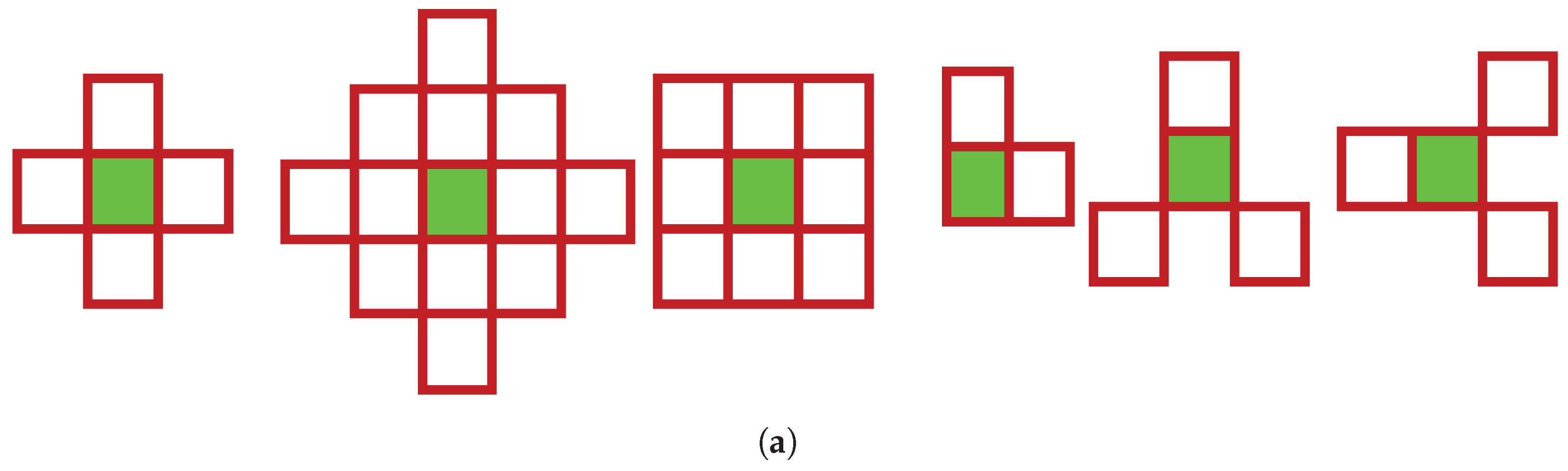
Figure 2.
The evolution of the two-dimensional cellular automaton in images according to the function with the von Neumann reference neighborhood, along the first 100 generations of 2D CA evolution for rule 9.
Figure 2.
The evolution of the two-dimensional cellular automaton in images according to the function with the von Neumann reference neighborhood, along the first 100 generations of 2D CA evolution for rule 9.
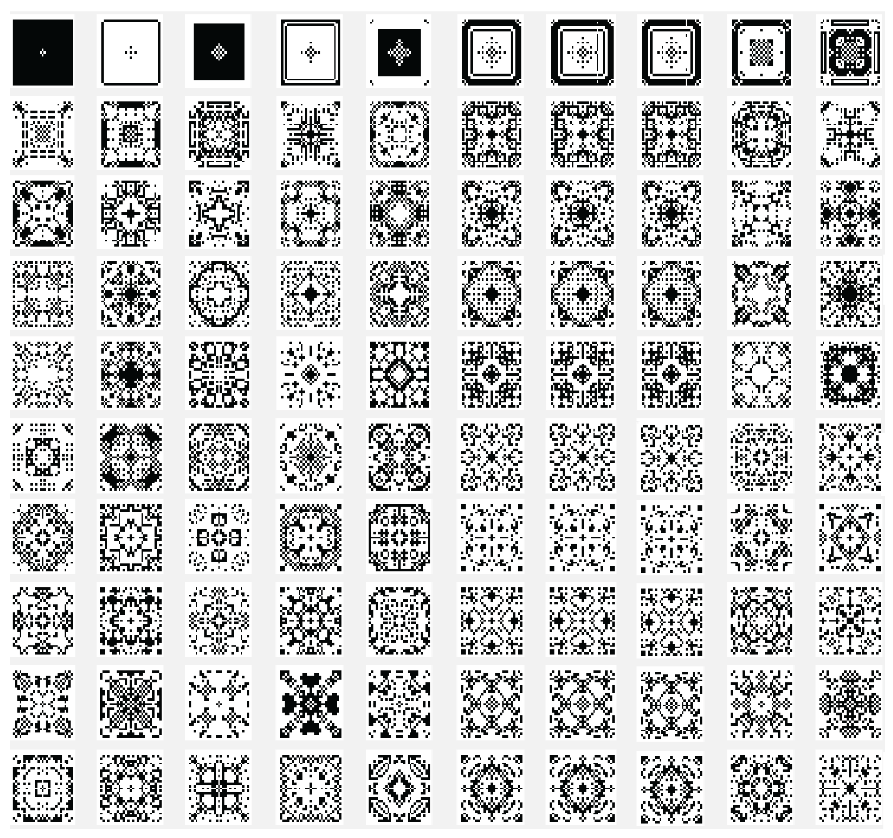
Figure 3.
The evolution of the two-dimensional cellular automaton in images according to the function with the von Neumann reference neighborhood, along the first 10 generations of 2D CA evolution for rules 6 (line 1), 9 (line 2), 17 (line 3), 21 (line 4), and 26 (line 5), respectively from the set .
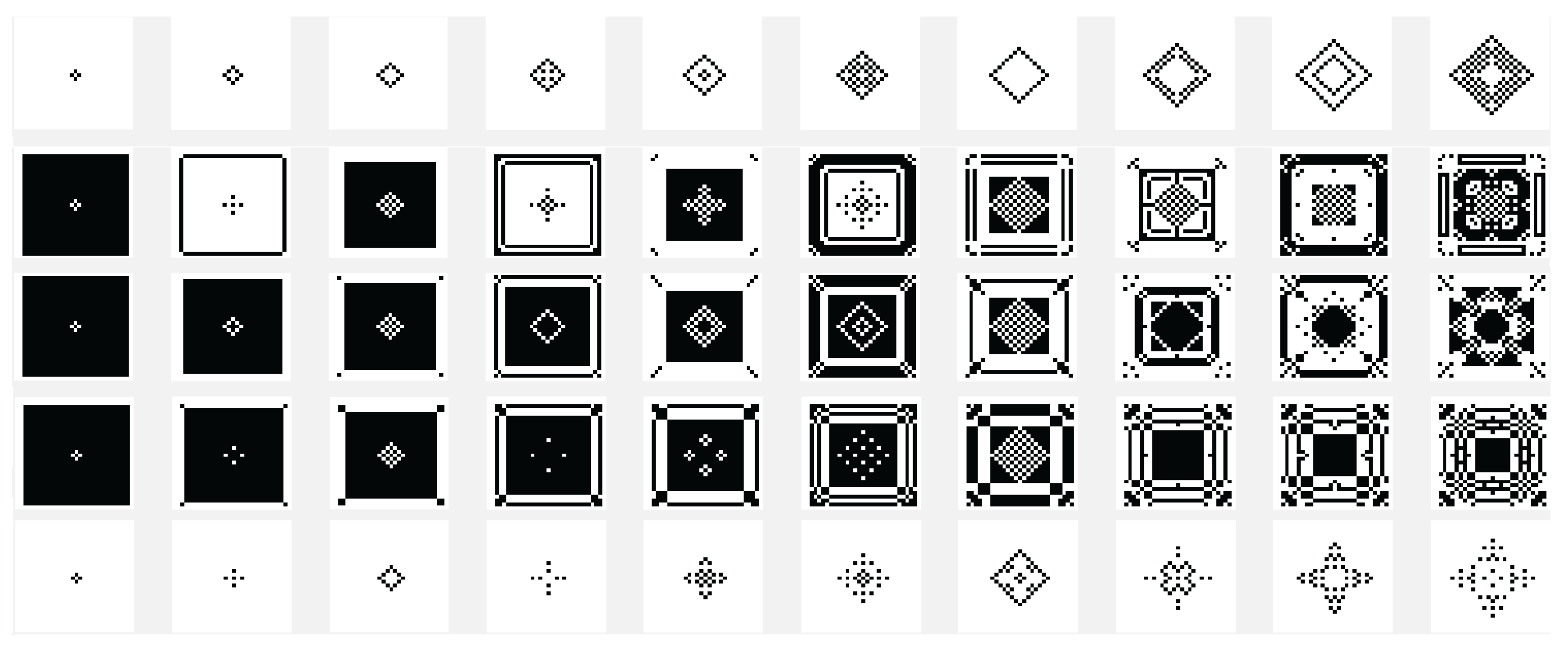
Figure 4.
The evolution of the two-dimensional cellular automaton in images according to the function with the von Neumann reference neighborhood, along generations of 2D CA evolution for rules 6 (line 1), 9 (line 2), 17 (line 3), 21 (line 4), and 26 (line 5), respectively from the set .
Figure 4.
The evolution of the two-dimensional cellular automaton in images according to the function with the von Neumann reference neighborhood, along generations of 2D CA evolution for rules 6 (line 1), 9 (line 2), 17 (line 3), 21 (line 4), and 26 (line 5), respectively from the set .
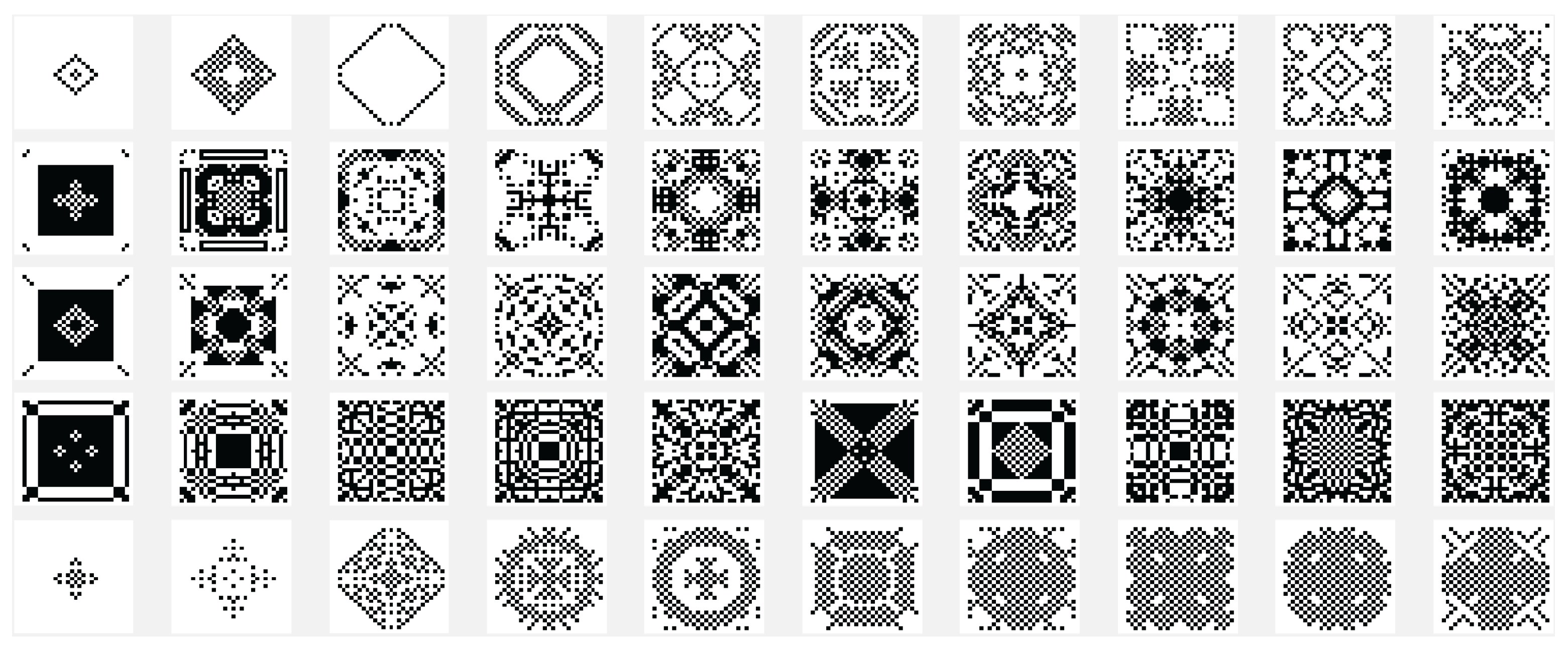
Figure 5.
The evolution of the two-dimensional cellular automaton in images according to the function with the Moore reference neighborhood with nine neighborhoods, along the first 100 generations of 2D CA evolution for rule 330
Figure 5.
The evolution of the two-dimensional cellular automaton in images according to the function with the Moore reference neighborhood with nine neighborhoods, along the first 100 generations of 2D CA evolution for rule 330
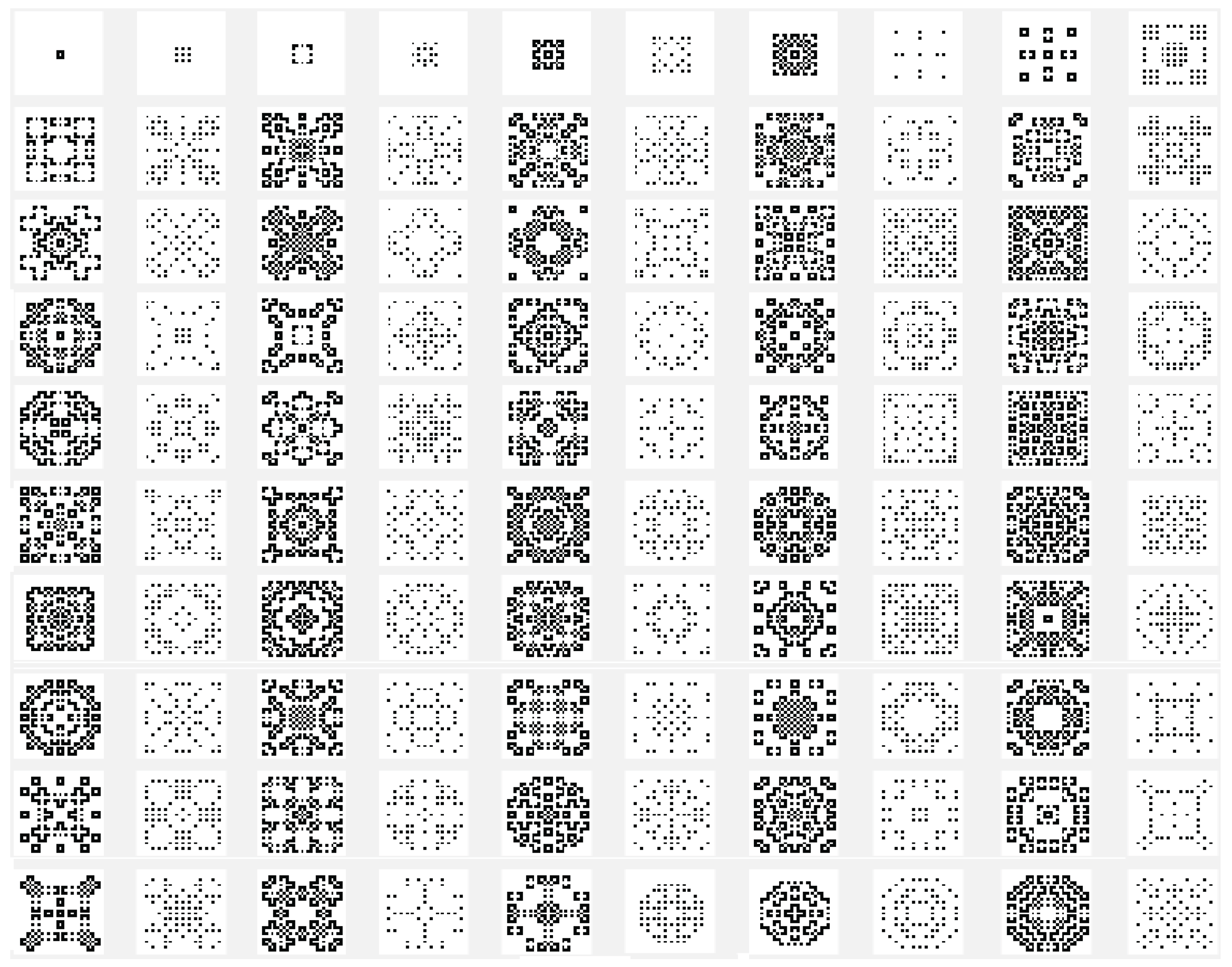
Figure 6.
The evolution of the two-dimensional cellular automaton in images according to the function with the Moore reference neighborhood with nine neighborhoods, along the first 10 generations of 2D CA evolution for rules 33 (line 1), 90 (line 2), 94 (line 3), 150 (line 4), 234 (line 5), 261 (line 6), 322 (line 7), 330 (line 8), 386 (line 9) and 490 (line 10), respectively from the set

Figure 7.
The evolution of the two-dimensional cellular automaton in images according to the function with the Moore reference neighborhood with nine neighborhoods, along generations of 2D CA evolution for rules 33 (line 1), 90 (line 2), 94 (line 3), 150 (line 4), 234 (line 5), 261 (line 6), 322 (line 7), 330 (line 8), 386 (line 9) and 490 (line 10), respectively from the set
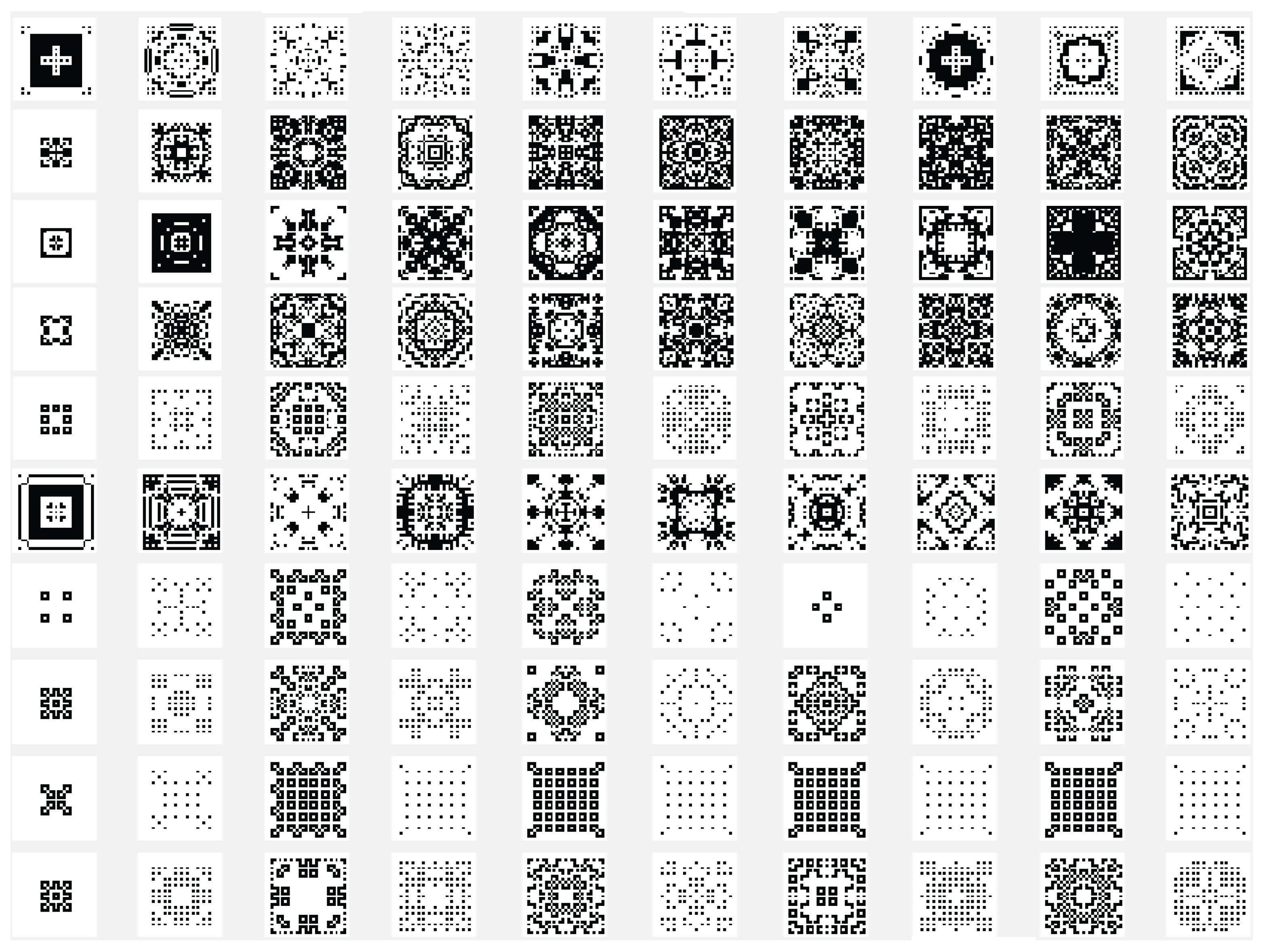
Figure 8.
The general structure of a GA which includes the stages of selecting chromosomes from the current population, recombining the selected chromosomes, carrying out some mutations on the resulting chromosomes and evaluating the quality of the new chromosomes through the fitness function that also determines the component of the new generation of chromosomes of the algorithm
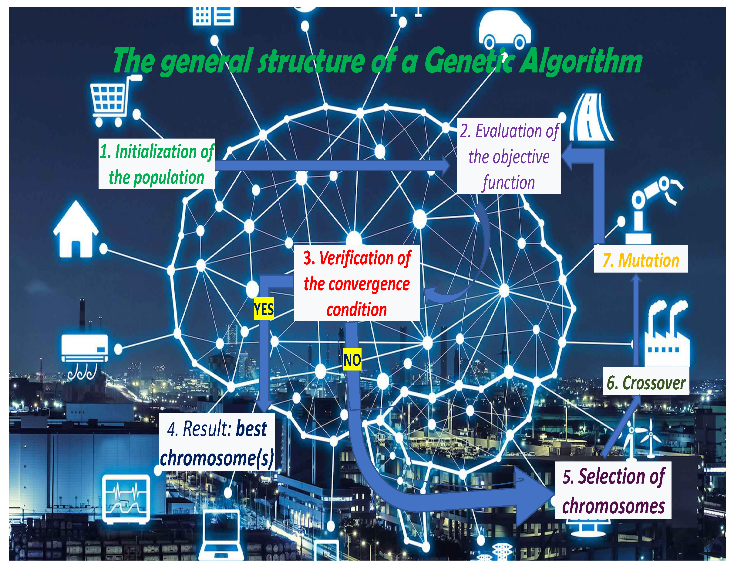
Figure 9.
Single-point crossover for two chromosome parents with genes with binary values and having the crossover point in position 3
Figure 9.
Single-point crossover for two chromosome parents with genes with binary values and having the crossover point in position 3
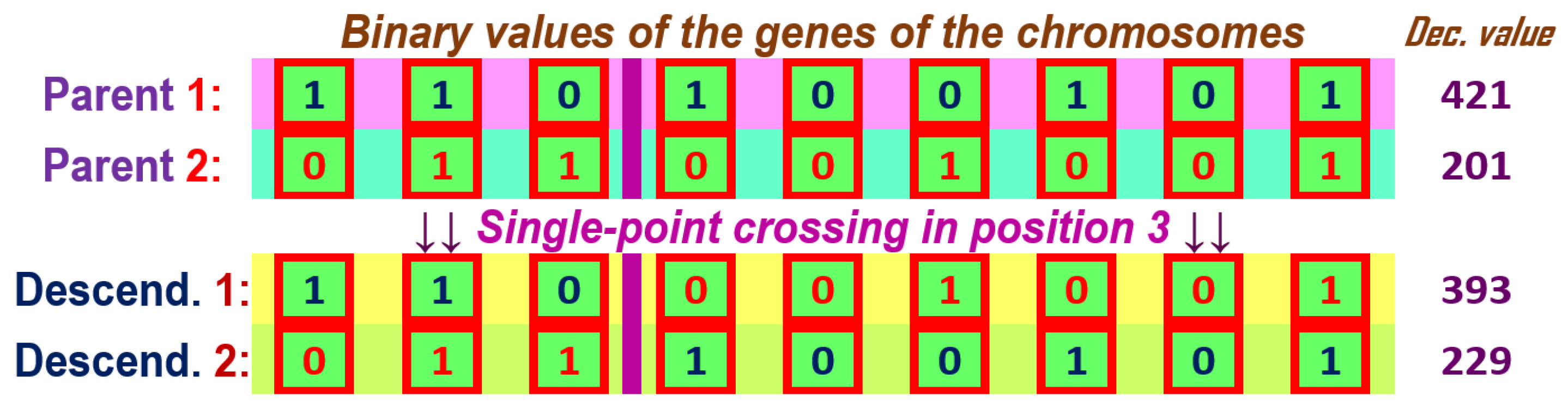
Figure 10.
Single-point crossover for two chromosome parents with genes with real values and having the crossover point in position 3
Figure 10.
Single-point crossover for two chromosome parents with genes with real values and having the crossover point in position 3
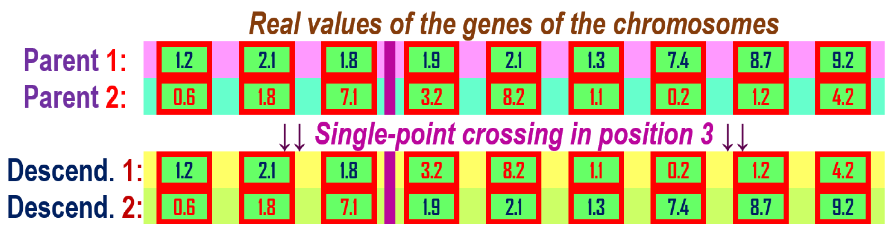
Figure 11.
k-point crossover for two chromosome parents with genes with binary values and having the crossover points in position 3, 5 and 7, k=3.
Figure 11.
k-point crossover for two chromosome parents with genes with binary values and having the crossover points in position 3, 5 and 7, k=3.
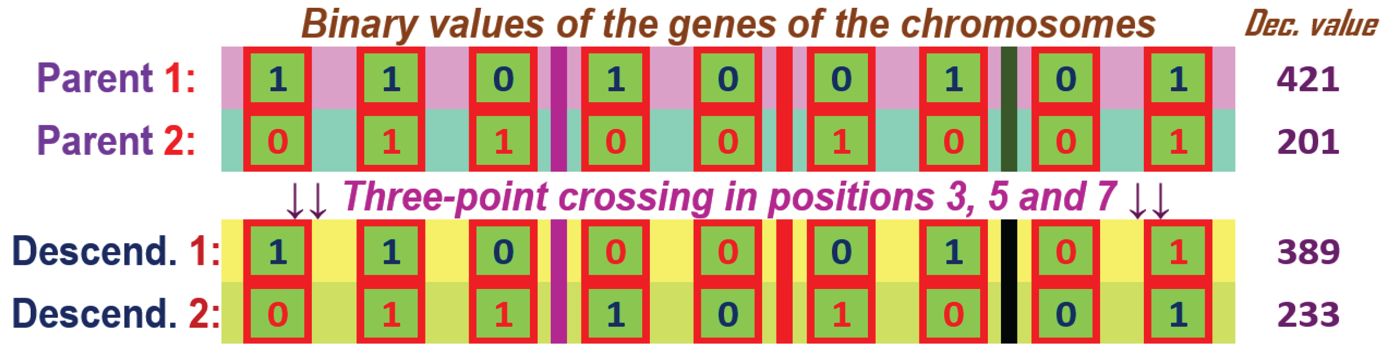
Figure 12.
k-point crossover for two chromosome parents with genes with real values and having the crossover points in position 3, 5 and 7, k=3.
Figure 12.
k-point crossover for two chromosome parents with genes with real values and having the crossover points in position 3, 5 and 7, k=3.
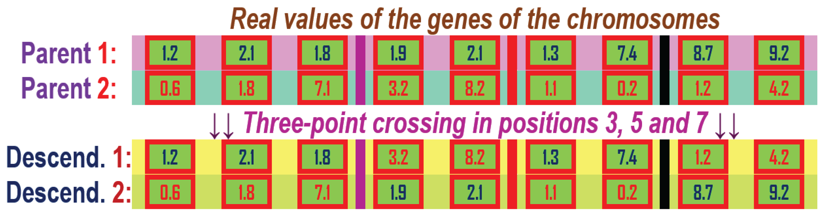
Figure 13.
The uniform crossover for two chromosome parents with genes with binary values and having the uniform parameter updating the genes at positions 4 and 7.
Figure 13.
The uniform crossover for two chromosome parents with genes with binary values and having the uniform parameter updating the genes at positions 4 and 7.
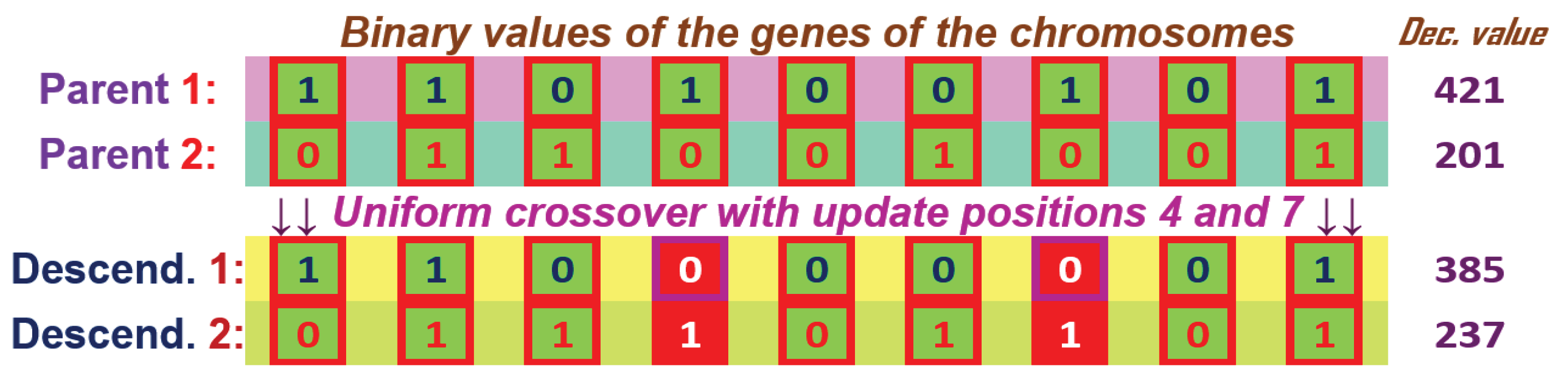
Figure 14.
The uniform crossover for two chromosome parents with genes with real values and having the uniform parameter updating the genes at positions 4 and 7.
Figure 14.
The uniform crossover for two chromosome parents with genes with real values and having the uniform parameter updating the genes at positions 4 and 7.

Figure 15.
The Partially-Mapped Crossover (PMX) for two parent chromosomes with 9 genes in the component and the parameters of the two cutting positions equal to 3 and 6.
Figure 15.
The Partially-Mapped Crossover (PMX) for two parent chromosomes with 9 genes in the component and the parameters of the two cutting positions equal to 3 and 6.
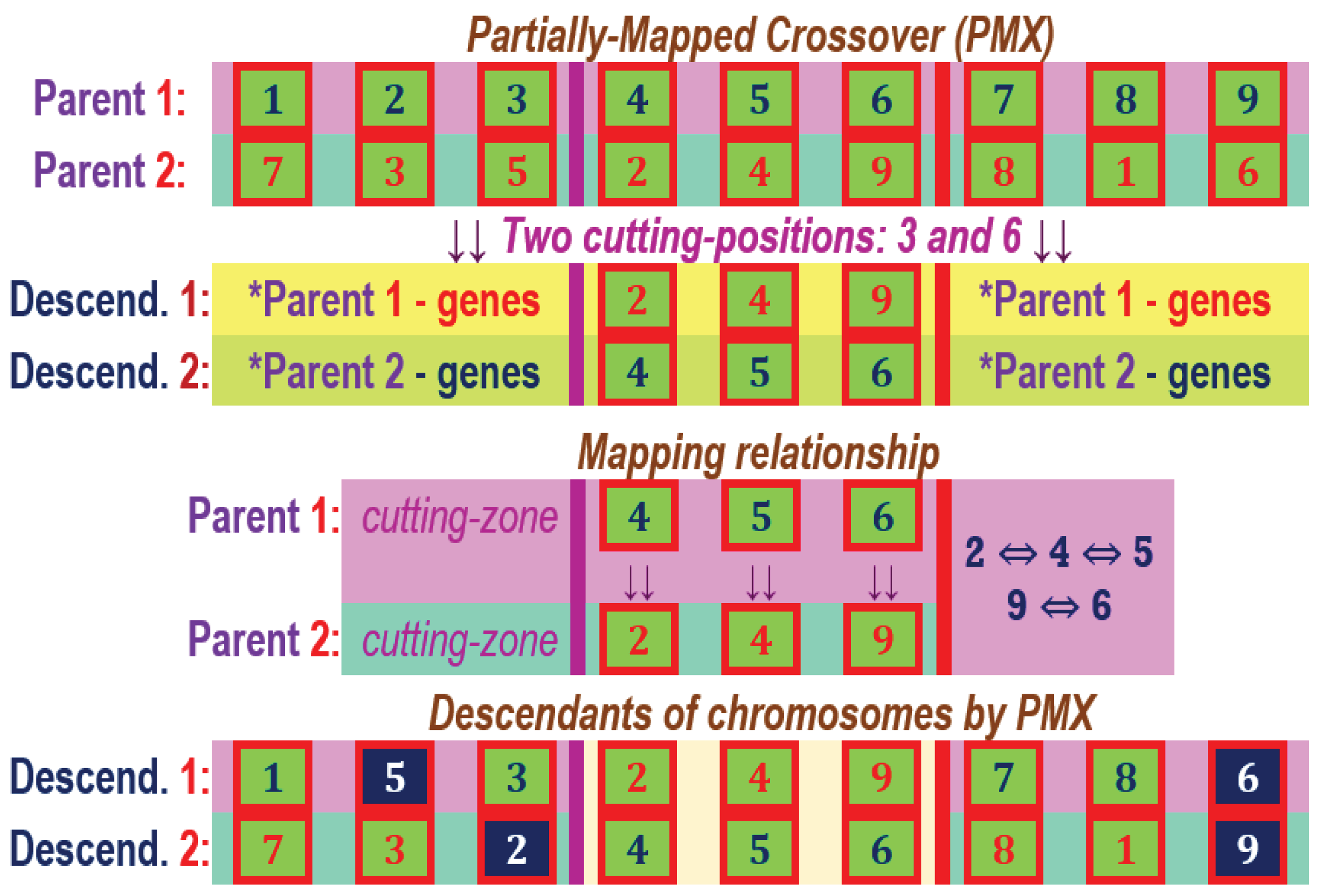
Figure 16.
The Order Crossover (OX) for two parent chromosomes with 9 genes in the component and the parameters of the four cutting positions equal to 2, 4, 6 and 7.
Figure 16.
The Order Crossover (OX) for two parent chromosomes with 9 genes in the component and the parameters of the four cutting positions equal to 2, 4, 6 and 7.
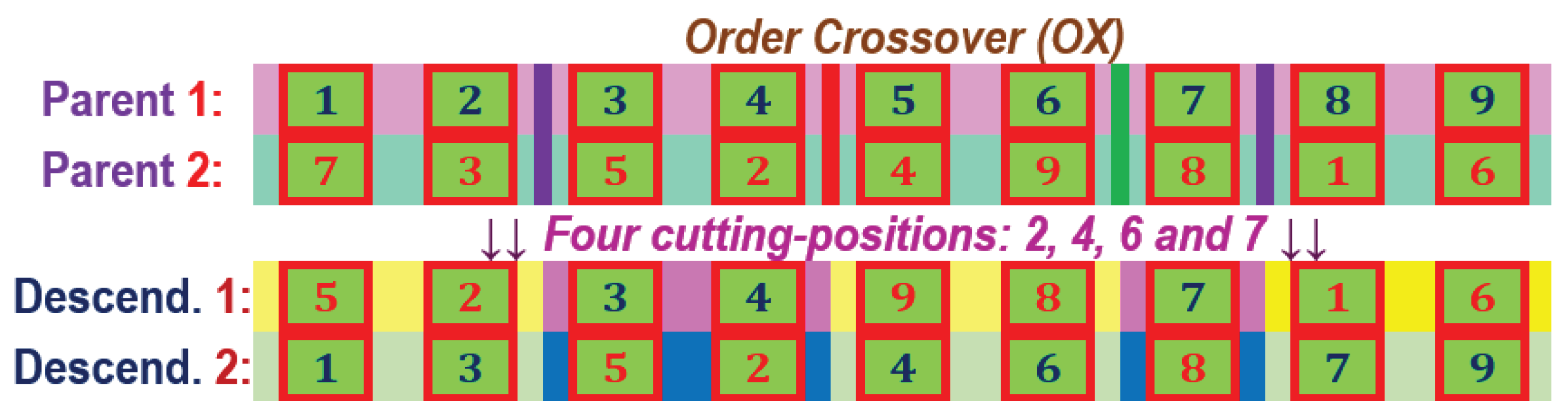
Figure 17.
The CGACell ECA Crossover for two parents with 9 genes by applying ECA Rule 110 at the individual chromosome level
Figure 17.
The CGACell ECA Crossover for two parents with 9 genes by applying ECA Rule 110 at the individual chromosome level
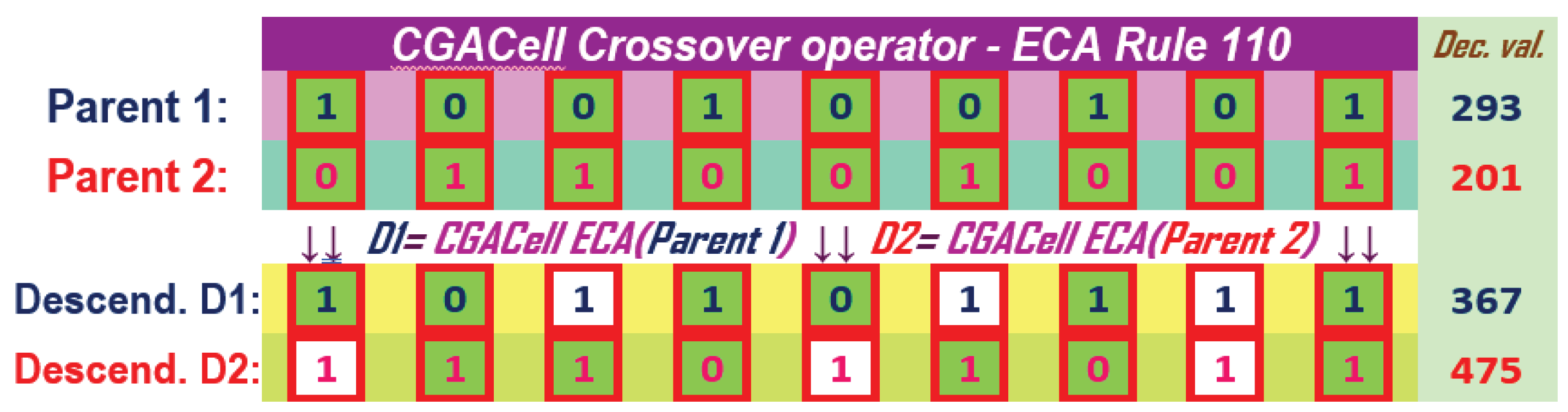
Figure 18.
The CGACell ECA Crossover for two parents with 9 genes by applying ECA Rule 90 at the individual chromosome level
Figure 18.
The CGACell ECA Crossover for two parents with 9 genes by applying ECA Rule 90 at the individual chromosome level
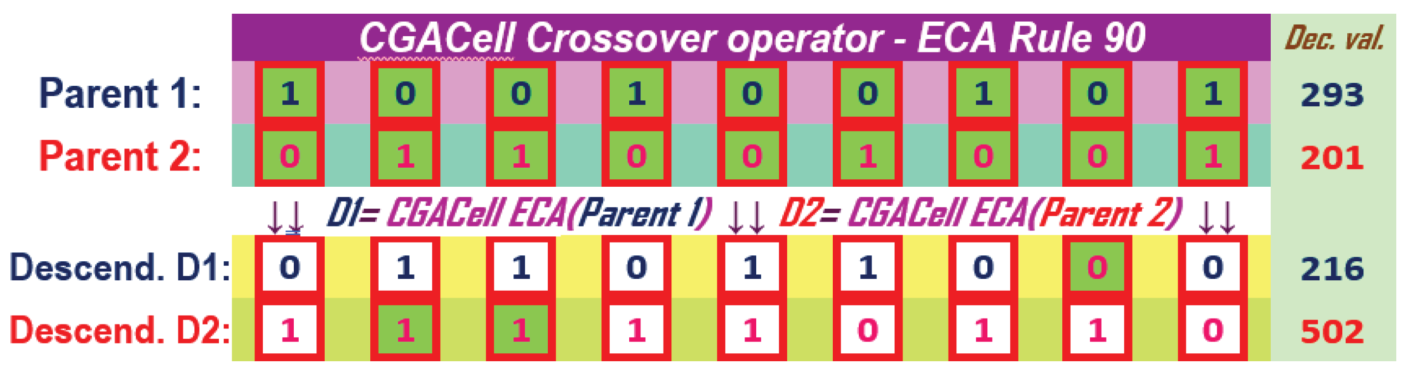
Figure 19.
The CGACell ECA Crossover in the mixed variant for three chromosomes with 9 genes by applying ECA Rule 110.
Figure 19.
The CGACell ECA Crossover in the mixed variant for three chromosomes with 9 genes by applying ECA Rule 110.
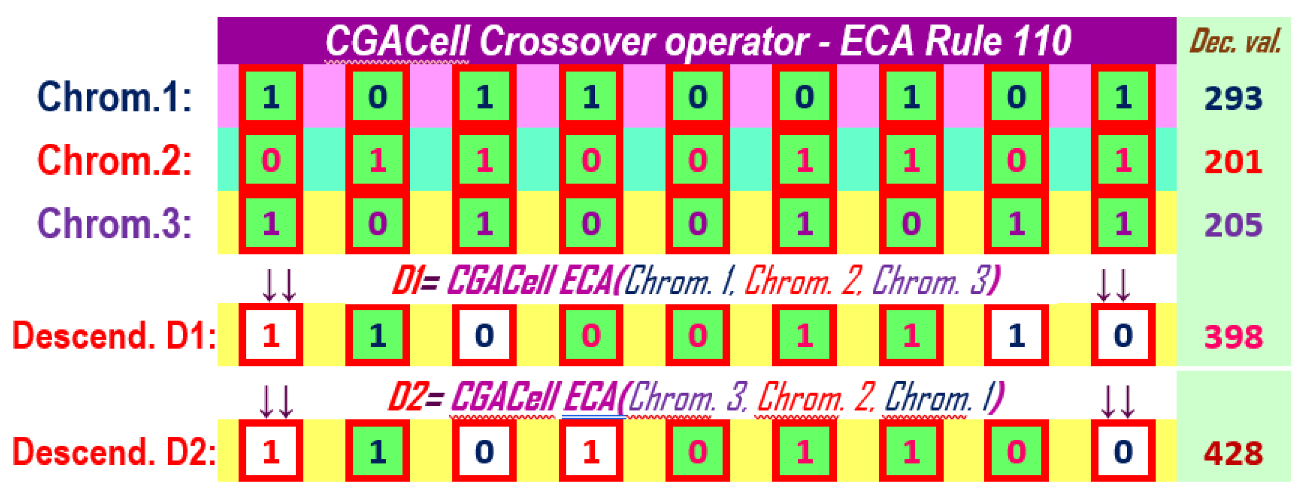
Figure 20.
The CGACell ECA Crossover in the mixed variant for three chromosomes with 9 genes by applying ECA Rule 90.
Figure 20.
The CGACell ECA Crossover in the mixed variant for three chromosomes with 9 genes by applying ECA Rule 90.
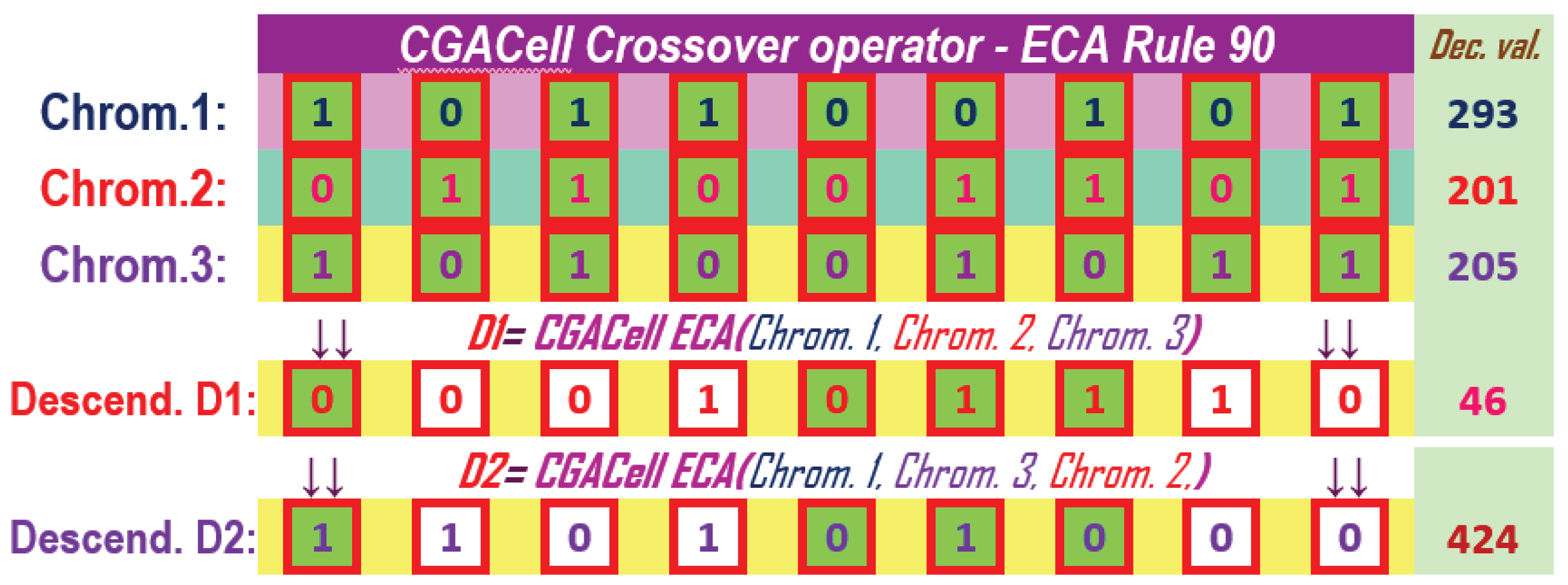
Figure 21.
The CGACell 2D CA Crossover for 10 chromosomes with 20 genes with von Neumann Neighborhood by applying 2D CA Rule 6.
Figure 21.
The CGACell 2D CA Crossover for 10 chromosomes with 20 genes with von Neumann Neighborhood by applying 2D CA Rule 6.
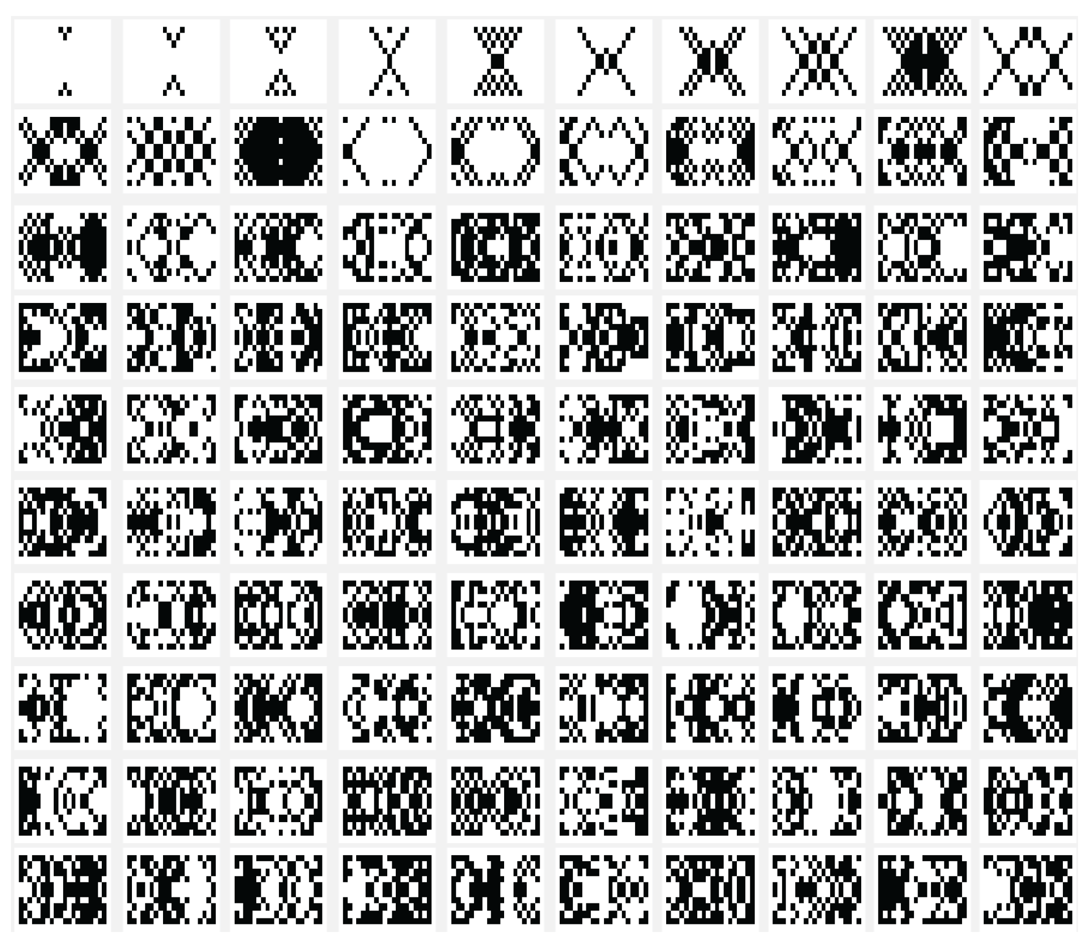
Figure 22.
The CGACell 2D CA Crossover for 10 chromosomes with 20 genes with von Neumann Neighborhood by applying 2D CA Rule 11.
Figure 22.
The CGACell 2D CA Crossover for 10 chromosomes with 20 genes with von Neumann Neighborhood by applying 2D CA Rule 11.
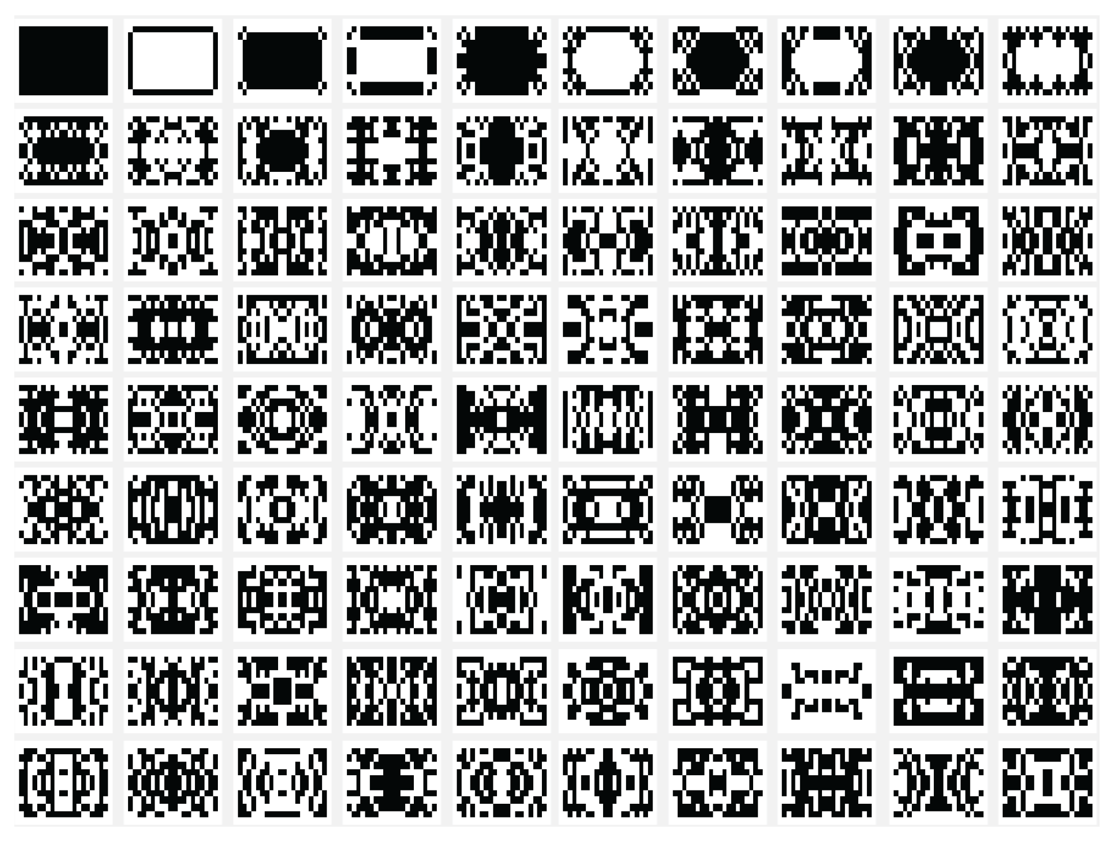
Figure 23.
The CGACell 2D CA Crossover for 10 chromosomes with 20 genes with Moore Neighborhood by applying 2D CA Rule 330.
Figure 23.
The CGACell 2D CA Crossover for 10 chromosomes with 20 genes with Moore Neighborhood by applying 2D CA Rule 330.
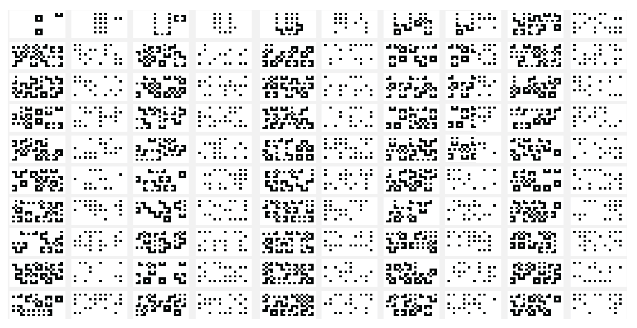
Figure 24.
The CGACell 2D CA Crossover for 10 chromosomes with 20 genes with Moore Neighborhood by applying 2D CA Rule 490.
Figure 24.
The CGACell 2D CA Crossover for 10 chromosomes with 20 genes with Moore Neighborhood by applying 2D CA Rule 490.
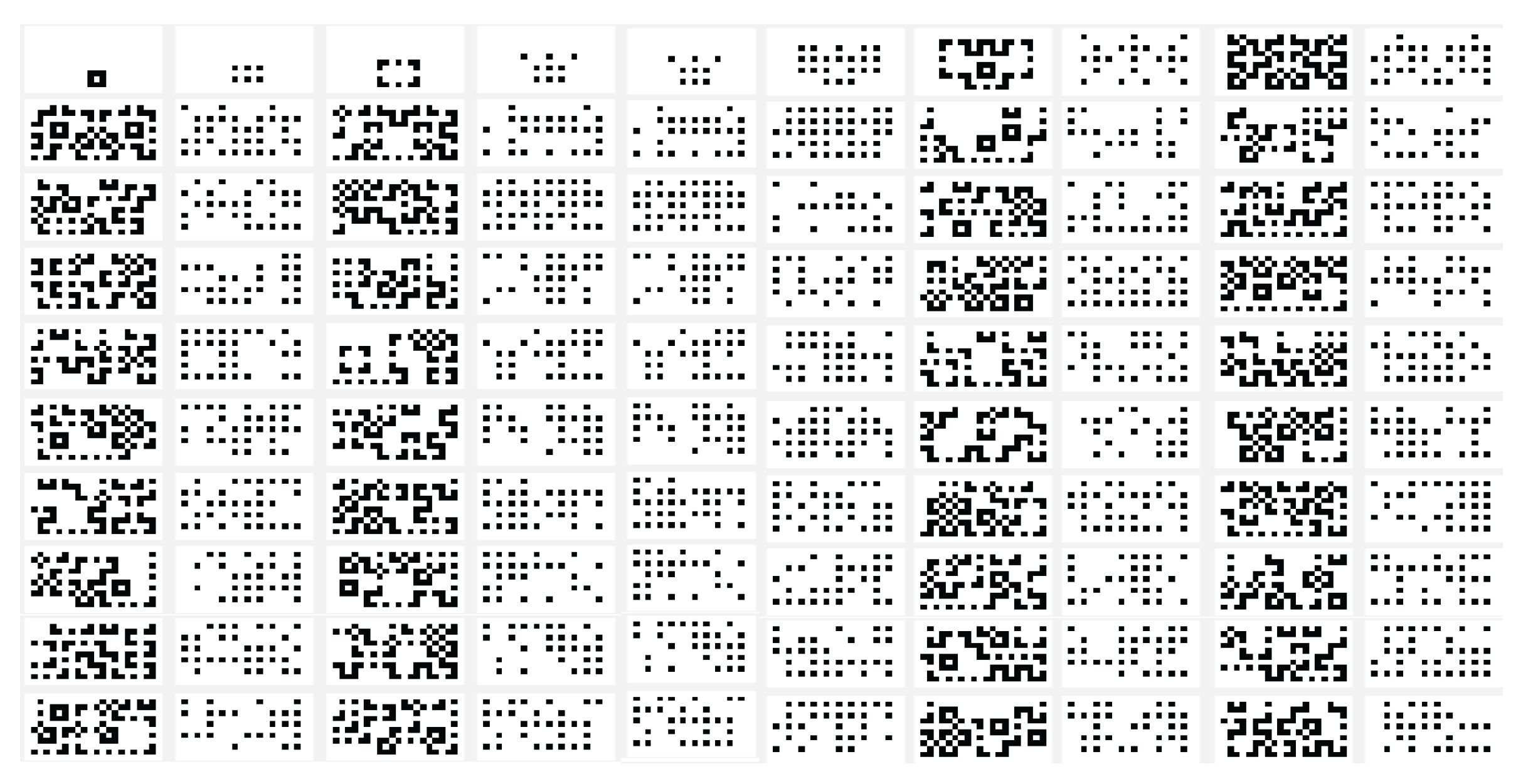
Figure 25.
Case I - Image classification for three face image classes from the Yale face database.
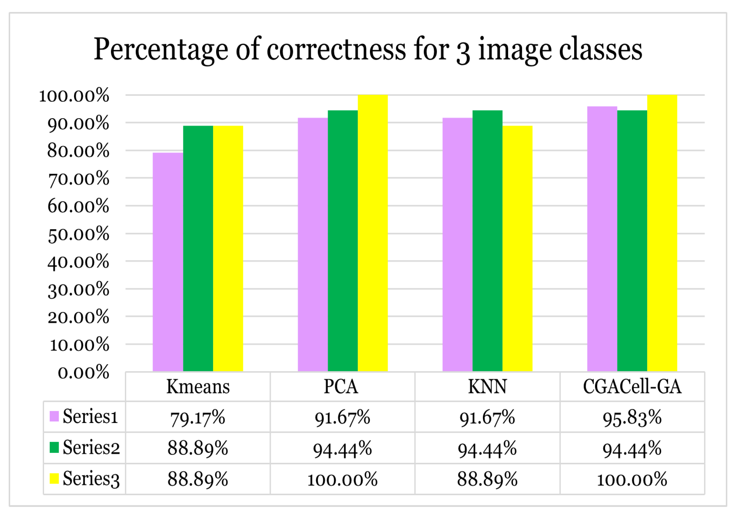
Figure 26.
Case II - Image classification for seven face image classes from the Yale face database.
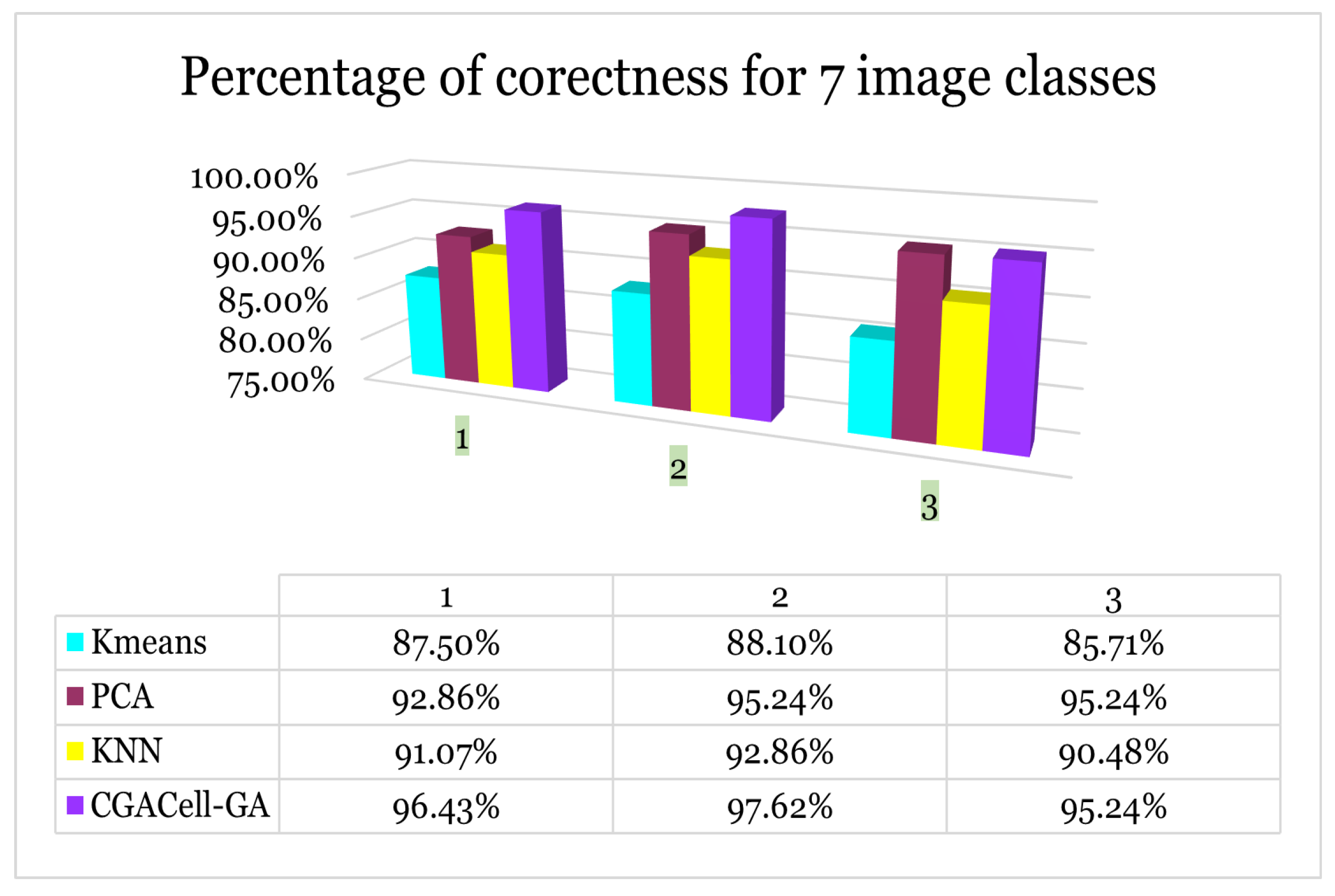
Figure 27.
Case III - Image classification for eleven face image classes from the Yale face database.
Figure 27.
Case III - Image classification for eleven face image classes from the Yale face database.
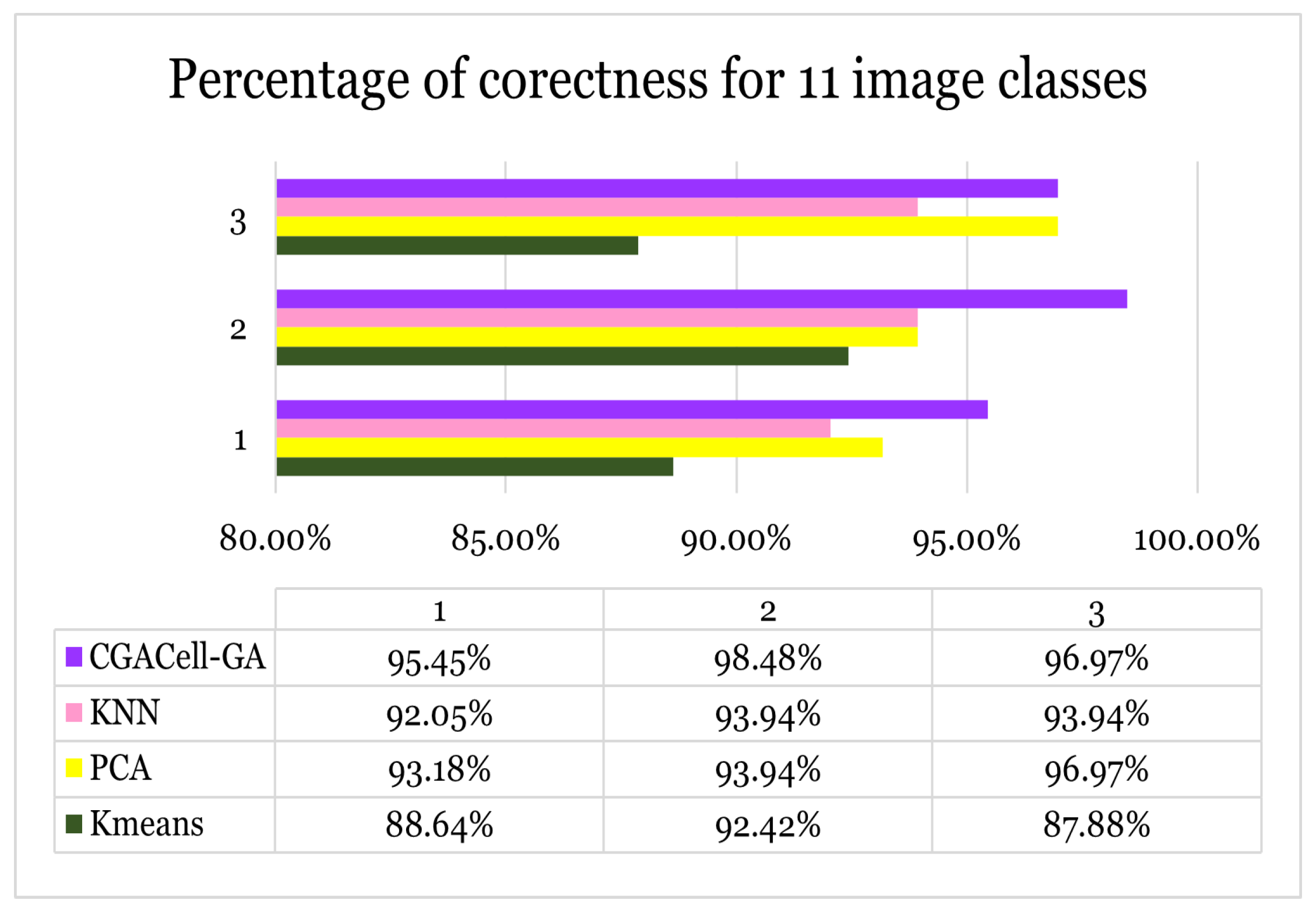
Figure 28.
Graphic representation of correct classification percents of face images for three, seven, and eleven classes of face images, respectively, and having three, five, and eight training images, respectively.
Figure 28.
Graphic representation of correct classification percents of face images for three, seven, and eleven classes of face images, respectively, and having three, five, and eight training images, respectively.
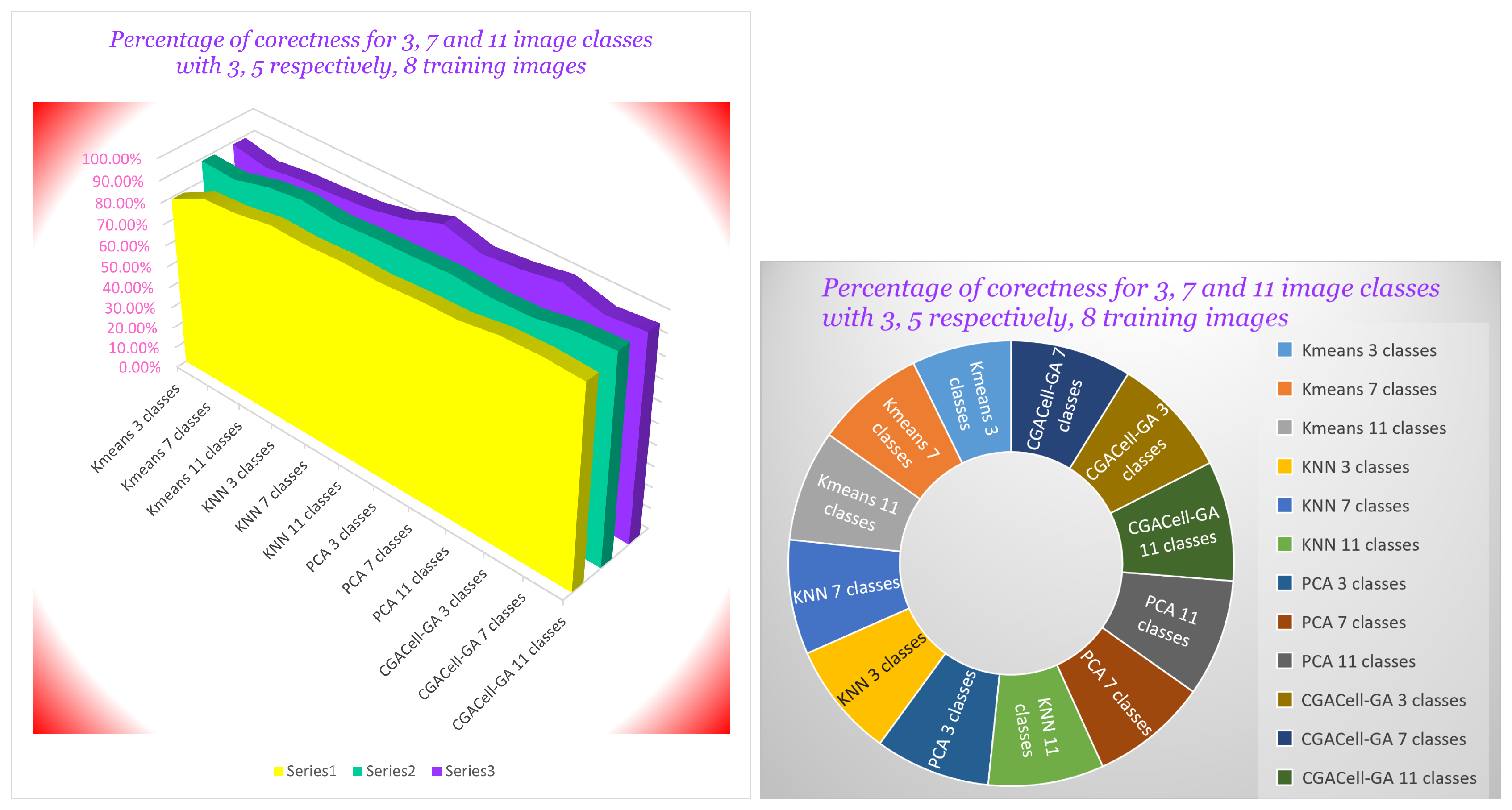

Table 1.
The elementary cellular automaton defined by Rule 110 of the Wolfram code.
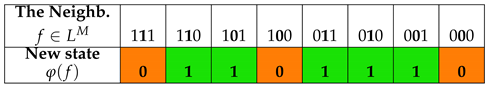
Table 2.
The elementary cellular automaton defined by Rule 90 of the Wolfram code.
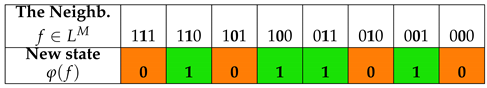
Table 3.
The results of ECA 110 for 10 generations with 16 cells.
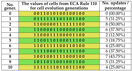
Table 4.
The results of ECA 90 for 10 generations with 16 cells.
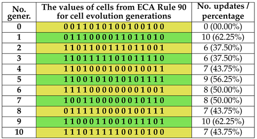
Table 5.
The binary images obtained after 150 generations with 31 cells used for ECAs 30, 90, 99, 110 and 158 - two images for each ECA having different initial sequences of cell state values.
Table 5.
The binary images obtained after 150 generations with 31 cells used for ECAs 30, 90, 99, 110 and 158 - two images for each ECA having different initial sequences of cell state values.
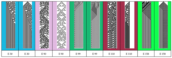
Table 6.
Values of correct classification percents of face images from the Yale database for three, seven, and eleven classes of face images, and having three, five, and eight training images
Table 6.
Values of correct classification percents of face images from the Yale database for three, seven, and eleven classes of face images, and having three, five, and eight training images
Disclaimer/Publisher’s Note: The statements, opinions and data contained in all publications are solely those of the individual author(s) and contributor(s) and not of MDPI and/or the editor(s). MDPI and/or the editor(s) disclaim responsibility for any injury to people or property resulting from any ideas, methods, instructions or products referred to in the content. |
© 2025 by the authors. Licensee MDPI, Basel, Switzerland. This article is an open access article distributed under the terms and conditions of the Creative Commons Attribution (CC BY) license (https://creativecommons.org/licenses/by/4.0/).
Copyright: This open access article is published under a Creative Commons CC BY 4.0 license, which permit the free download, distribution, and reuse, provided that the author and preprint are cited in any reuse.


