
Submitted:
10 July 2025
Posted:
10 July 2025
You are already at the latest version
Abstract
Underestimation of PM2.5 emissions from the agricultural sector persists as a major difficulty for air quality studies, partly because of underutilization of high-resolution observation platform for constructing a global emissions inventory. Coarse-resolution products used for such purpose often miss fine-scale burnt areas created by stubble burning practices, which are primary sources of agricultural PM2.5 emissions. For this study, we used the high-resolution Sentinel-2 observations to examine the spatiotemporal variability of burnt areas in Punjab, a major hotspot of agricultural burning in India, during the post-monsoon fire season (October–December) in 2022–2024. The results highlight the Sentinel-2 capability of detecting more than 34,000 km2 of burnt areas (approx. 68% of Punjab’s total area) as opposed to the less than 7,000 km2 (approx. 12% of Punjab’s total area) detected by MODIS. The study also reveals, in unprecedented detail, multi-annual spatial and temporal shifting of burning events from northern to central and southern Punjab. This detection discrepancy has led to marked disparities in estimated monthly emissions, with approximately 427.5 million tons of PM2.5 emitted in October 2022 compared to 8.7 million tons found by EDGAR v.8.1, underscoring higher resolution observation systems intended to support construction of a global PM2.5 emissions inventory.
Keywords:
burn severity
; burnt area detection
; dNBR
; fire radiative power
; google earth engine
; MODIS
; normalized burn ratio
; PM2.5 emission
; sentinel-2
1. Introduction
Stubble burning is a practice of setting fire to the remaining straw stubble in a cultivated field after the grain or main product has been harvested. Although outcomes are similar, stubble burning is differentiated from wildfires because of the intentional nature of the former and its primary scope of application to the agricultural sector. Despite its benefits as a quick, cheap, and efficient method to prepare soil beds for later crops, stubble burning has been banned in many countries around the globe for decades. In fact, this practice has been cited as a major cause of air pollution and as a driver of climate change by releasing huge quantities of greenhouse gases to the atmosphere [1,2].
For the last two decades, stubble burning in Punjab has emerged as a major environmental issue in India. For instance, post-harvest stubble burning in November engenders nearly 43% aerosol loading over the populous Indo-Gangetic Plain [3]. A recent study revealed that, based on annual particulate matter 2.5 (PM2.5) rankings by city, 35 of the top 50 most polluted cities in the world are in India [4]. Most states, and 76.8% of the population, are exposed to annual population-weighted mean PM2.5 greater than 40 μg/m3, which is the limit recommended by Indian National Ambient Air Quality Standards [5,6]. Air pollution, which has affected the health of Indian residents, has increased mortality and morbidity rates nationwide. In 2017, 1.24 million deaths, fully one-eighth of all deaths recorded in India, were attributed to air pollution, approximately half of which were people younger than 70 years old [5].
For decades, satellite-based remote sensing has been used as a powerful tool for monitoring and detecting physical characteristics over the land, air, and ocean on regional and global scales [7]–[10]. Remote sensing has been used specifically for mapping and planning [11]–[13], weather monitoring [14] and change detection [15,16]. Utilization of remote sensing has proven useful for assessing effects of anthropogenic intervention and landscape changes on the environment, such as those to natural vegetation and hydrological ecosystems [17]. Another popular application of remote sensing technology for change detection is for the monitoring and forecasting of wildfires. Various indices such as Normalized Difference Vegetation Index (NDVI) and Normalized Difference Water Index (NDWI) have been developed to evaluate the relation between remote sensing derived variables and fire danger-related indicators [18]. Vast coverage and data availability of remote sensing observation can be combined further with in-situ observation or static datasets to improve fire forecasting system performance [19]. These sophisticated systems can be improved even further by combining them with state-of-the-art technology such as machine learning and internet of things (IoT) [20,21]. It is noteworthy, however, that most fire monitoring and forecasting systems are using remote sensing observation in the moderate range and coarse spatial resolution.
The Moderate Resolution Imaging Spectrometer (MODIS) and Visible Infrared Imaging Radiometer Suite (VIIRS) have been used particularly and widely for fire monitoring systems, especially to detect active fire hotspot (FHS) and burnt areas, which are the main sources of air pollution [7,8,22,23]. Subsequently, the FHS information from these observations is used to construct global fire emission inventories, which are fundamentally important for models of atmospheric composition to reconstruct and project the effects of biomass burning on the air quality, public health, ecosystem dynamics, climate, and land–atmosphere exchanges [24]. The coarse resolution of MODIS and VIIRS products however, renders them ineffective for the detection of fire hotspots smaller than their grid cells, which engenders underestimation of the total burnt area and erroneous simulation of aerosol emissions over the target region [24,25].
As described herein, we demonstrated the capabilities of Sentinel-2 [26] observations to examine the spatiotemporal variability of stubble burning activity in the state of Punjab, northern India, during post-monsoon fire seasons across the three consecutive years of 2022–2024. Numerous studies have been undertaken during the past 15 years to monitor burnt areas in India. Research using data from advanced wide field sensor (AWiFS) observations has been reported for the Punjab region in 2005, yielding estimation of the extent of burnt areas and greenhouse gas (GHG) emissions from crop residue burning [27]. Similar attempts have been undertaken using fine resolution images of LISS III and Landsat 8 Operational Land Imager (OLI) satellites in 2007 and 2014–2018 [28,29]. Using data from these fine-resolution observations enables burnt area mapping in high detail and with high accuracy, but cloud obstruction and low revisiting frequencies of these satellites have posed difficulties for temporal analysis and prediction, thereby prompting scholars to use data from observations with coarser spatial resolution but with higher revisit frequency [30].
In contrast to MODIS and VIIRS, which were typically used by global fire emission inventories, the high-resolution and five-day revisiting frequency of Sentinel-2 (with two satellites) enable the use of composite images to detect burnt scars left after stubble burning activities, to reduce the obscuring effects of clouds and aerosols, and to detect surface changes with greater detail and higher accuracy. Moreover, the versatility of Sentinel-2 observations has been extended recently by incorporation of machine learning technology to improve the accuracy of burnt area assessment over Punjab [31]. For this study, we opt to use Sentinel-2 observation for burnt area detection using a consistent, interpretable and operationally efficient method of the differenced Normalized Burn Ratio (dNBR), which has proven reliable for capturing areas scarred by burning over various land surfaces [32]. Unlike machine learning approaches, which often require large, spatially diverse training datasets and complex interpretability, the dNBR method offers a physically meaningful index that can be applied easily for large areas and multiple time periods, making it suitable for examining the temporal dynamics of stubble burning to support regional fire management efforts.
Furthermore, we implemented this study using Google Earth Engine (GEE), a state-of-the-art cloud computing platform, which provides access to an extensive geospatial data catalog along with on-the-fly computation for analyzing dynamic changes in agriculture, natural resources, and climate [33]. The GEE allows users to collaborate using data, algorithms, and visualization, thereby enabling this study to be implemented easily in the future, either for research or operational purposes (e.g. monitoring and prediction).
2. Materials and Methods
2.1. Area of Interest
This study specifically examines the state of Punjab, India, with total area of 50,225 km2 and located between 29° 33’N and 32° 30’N, 73° 53’E and 76° 54’E, as shown in Figure 1. This region is well known as a main producer of wheat and rice for the country. Moreover, it has been reported repeatedly in recent years as a major hotspot for stubble burning, a practice commonly adopted by farmers to clear rice residue quickly in preparation for the subsequent wheat crop [2,34]. The agricultural calendar in Punjab typically involves sowing rice (Kharif crop) in May–June, with harvesting during October to mid-November. Immediately thereafter, wheat (Rabi crop) is sown for the winter, which extends from November through April; it is harvested during April–May. This tight cropping cycle allows only a brief window of 10–15 days for field preparation between the rice harvest and wheat sowing. Because of the time and economic constraints, burning of crop residues remains a widely adopted method for land clearing [35,36]. Based on this fact, our study targets the post-monsoon fire season (October–December) during three consecutive years: 2022, 2023, and 2024. That period typically coincides with intense stubble burning activity.
2.2. Data
The workflow of this study is presented in greater detail in Figure 2. To investigate the spatial and temporal characteristics of burnt areas in Punjab, we used high-resolution satellite imagery and conducted a comparative analysis using multiple datasets that are freely available on the Google Earth Engine (GEE) platform (https://earthengine.google.com). Burnt area (BA) detection in this study was conducted using Sentinel-2 Surface Reflectance (S2 SR) imagery acquired from the COPERNICUS/S2_SR_HARMONIZED collection. The dataset provides atmospherically corrected surface reflectance values at spatial resolution of 10–20 m across 13 spectral bands. Images of October–December during 2022–2024 are selected corresponding to the post-monsoon fire season in Punjab. Cloud-contaminated pixels were removed using a combination of the Scene Classification Layer (SCL) and the Sentinel-2 cloud probability dataset (COPERNICUS/S2_CLOUD_PROBABILITY). Specifically, pixels which are classified as cloud, cirrus, or shadow in the SCL were masked out. Then an additional threshold of cloud probability > 70% was applied to exclude high-confidence cloudy pixels.
To ensure that calculations were restricted to agricultural areas, the ESA WorldCover 10m 2021 land cover (ESA/WorldCover/v200/2021) dataset was used to mask non-cropland classes. Only pixels classified as cropland (class value 40) were retained: all other land cover types were excluded from the analysis.
To support the analysis and to provide a broader perspective, we also used MODIS active fire data from both the MOD14A1 (Terra) and MYD14A1 (Aqua) products, which are available on MODIS/061/MOD14A1 and MODIS/061/MYD14A1 collections. These products provide fire pixel detections at 1 km spatial resolution based on thermal anomalies. Fire detection data from both satellites were aggregated over the same two-week periods for comparison with Sentinel-2-derived BA maps.
As a qualitative validation step, we used geo-referenced field photographs of confirmed locations that had been burnt in Ludhiana district, Punjab. The photographs, which had been taken on October 30 and November 6, 2022, were matched with the corresponding Sentinel-2 BA maps to confirm the BA detection accuracy visually. Although field-based observations were only available for part of the study period, they provide valuable evidence supporting the spatial validity of the spectral-based approach used for this study.
To assess the broader atmospheric effects of burning activity, PM2.5 emissions estimated from Sentinel-2-derived burnt areas were compared with anthropogenic PM2.5 data from Emissions Database for Global Atmospheric Research (EDGAR) v.8.1 (https://edgar.jrc.ec.europa.eu/dataset_ap81) global emission inventory, which provides gridded emissions from 1970–2022 at spatial resolution of 0.1° × 0.1°. EDGAR offers sector-specific and total PM2.5 emissions at a global scale, which facilitates direct comparison between satellite-based fire-related estimates and reported anthropogenic emissions over Punjab during the most recent overlapping year.
2.3. Identification of Burnt Areas
2.3.1. Sentinel-2 dNBR
To identify BA over northern India, the Normalized Burn Ratio (NBR) has been used. The NBR index has also been used for several studies [25,29,37]. Reportedly, as an excellent method for assessing burnt areas [38,39], this index can map burnt areas effectively for many different landscapes worldwide using its near infrared (NIR) and short wave infrared (SWIR) bands. The burnt area extent can be estimated by exploiting the distinction between spectral responses of healthy vegetation. A high NBR value represents healthy vegetation, whereas a low value represents bare ground and areas affected by recent burning. The NBR index is calculated using the following equation.
(1)
The NIR band of Sentinel-2 (Band 8) includes wavelengths of 835.1 nm (Sentinel-2A) and 833 nm (Sentinel-2B). Sentinel-2 provides two SWIR bands (Band 11 and 12) with identical resolution (20 m). However, for this study, we chose Band 12 of Sentinel-2, which has longer wavelength (2202.4 nm and 2185.7 nm) than Band 11 (1613.7 nm and 1610.4 nm), to achieve better spectral response for the burnt areas. The difference between prefire and postfire NBR obtained from the images is used to calculate the delta NBR (dNBR or ∆NBR). A higher value of dNBR represents more severe damage, whereas areas with negative dNBR values might denote regrowth following a fire. The formula used to calculate dNBR is presented below.
(2)
A time series of dNBR values can be generated by calculating the NBR indices for certain prefire and postfire periods, for instance, at weekly or monthly intervals. For an interval i, the formula can be rewritten as presented below.
(3)
The tight schedule between the harvest and sowing periods in northern India, especially in Punjab, engenders rapid changes over the land surface. For that reason, using an interval longer than two weeks might hinder burnt area detection. However, using a shorter time interval might engender more missing scenes in the composites. To avoid such outcomes, we examined the burn severity variation during a two-week interval: days 1–15 and 16 to the end of the month, resulting in intervals of 16–31 for October and December, and 16–30 for November. A threshold of dNBR ≥ 0.1 was applied to classify pixels as burnt [32]. For this study, we exclusively emphasize burnt areas and therefore consider dNBR values below 0.1 as unburnt, without accounting for post-fire vegetation growth. The burn severity values calculated from dNBR for this study are presented in Table 1.
2.3.2. MODIS Fire Hotspot
Hotspot data were retrieved by filtering daily MODIS fire detections to include only pixels with a “nominal” confidence level, based on the confidence flag provided in the MOD14A1 (Terra) and MYD14A1 (Aqua) products. The “nominal” confidence class offers a practical balance: it includes detections that are reasonably reliable without excluding moderate-intensity fires; such detections are common in cropland burning scenarios such as those observed in Punjab. Using only the nominal category, we reduced false positives while preserving a representative dataset of actual fire activity that is suitable for comparison with Sentinel-2-derived burnt area patterns.
The data were constrained spatially to the Punjab region and were temporally limited to the October–December period during 2022–2024, which aligns with the S2 SR observation window. Detections from both Terra and Aqua were then merged and aggregated into two-week intervals, corresponding to the compositing periods used for the Sentinel-2 analysis. The total BA derived from MODIS was then estimated by multiplying the number of active fire pixels by the nominal spatial resolution of 1 km2 per pixel, while assuming that each instance of fire detection represents at least one square kilometer of BA. This estimate, which provides an upper-bound approximation of fire-affected surfaces, was used to compare temporal patterns and magnitudes of BA between MODIS and Sentinel-2 datasets.
2.4. Estimated PM2.5 Emissions
To estimate PM2.5 emissions from agricultural burning, we applied the emission factor (EF) approach, which calculates emissions as the products of BA, available fuel load (biomass), and pollutant-specific emissions factors. The total emissions were computed as presented below.
(4)
In that equation, BAkm2 denotes the Sentinel-2-derived BA in square kilometers, B represents the effective dry biomass loading in kilograms/m2, and EF is the emission factor in kilograms of PM2.5 per kilogram of dry biomass that is burnt.
Because rice is the dominant crop in the region, parameter values were selected accordingly. The dry biomass loading for rice residues is typically 4.2–8.0 t/ha (0.42–0.80 kg/m2), depending on local agronomic practices [40,41]. A midpoint value of 1.2 kg/m2 was adopted. With an assumed burning efficiency of 80%, the effective fuel load was set as 0.96 kg/m2. The EF for PM2.5 was taken as 9.1 g/kg (0.0091 kg/kg), which is consistent with measurements for open-field rice straw burning in Southeast Asia [42,43]. This EF value lies within the reported range of 4.2–20.7 g/kg for rice residue combustion. Because the burnt area was derived at a two-week temporal resolution, biweekly PM2.5 emissions estimation was adopted. This estimation allowed us to construct a two-weekly time series of emissions, enabling more detailed assessment of emission dynamics during the peak burning season (October–December).
To assess the representativeness of PM2.5 emissions estimated from Sentinel-2-derived burnt areas, we compared them with anthropogenic emissions from the EDGAR v.8.1. We specifically used the agricultural waste burning sector of the EDGAR dataset, which provides globally consistent, gridded annual emissions of greenhouse gases and air pollutants, including PM2.5. EDGAR emissions are derived using the EF approach, by which total emissions are calculated as the product of activity data (AD) and sector-specific EFs, following guidelines from the Intergovernmental Panel on Climate Change (IPCC). These calculations are harmonized across countries using internationally reported data and are allocated spatially using geospatial proxies.
For comparison with our Sentinel-2 results, we extracted EDGAR PM2.5 emission data for the Punjab region for 2022, which is the latest year currently available. Although EDGAR emissions represent anthropogenic fire activity at national scale, they provide a useful reference for evaluating the magnitude and spatial pattern of PM2.5 released from agricultural burning, as inferred independently from high-resolution satellite-derived burnt area data.
3. Results
3.1. Burnt Area Detection from Sentinel-2
Figure 3 portrays histograms constructed from two-weekly dNBR values across Punjab during October–December in 2022–2024. Each histogram reveals a dominant unimodal pattern of dNBR values for each period of observation. Across all three years, the October 1–15 curves have a peak near zero, suggesting minimal or no burning. However, in later periods (November–December), the histograms flatten and shift rightward with increased dNBR values, indicating the emergence of burn signals. The histograms for 2022 and 2023 have more pronounced right-side tails in November–December curves compared to 2024, which suggests a higher frequency of moderate to high burn severity during those years. The 2024 curves (especially November 16–30) show a less steep rise beyond 0.1, which might indicate lower fire intensity or coverage. By contrast, the 2024 November 16–30 curve represents the only period among those of the same observation time during which dNBR primarily shifts towards values larger than the 0.1 threshold, indicating a prolongation of severe burn signals compared to earlier years. Figure 3 also shows that the 0.1 dNBR threshold line intersects the histograms near the inflection point where the frequency starts declining which indicates that the threshold is empirically reasonable to separate unburnt and burnt areas.
Figure 4(a)–4(c) show the BA maps derived from the dNBR values across Punjab for each two-weekly period of observations. Across all three years, fire activity consistently begins in early October with scattered low-severity burns (dNBR approx. 0.1, green), primarily in the northern and central parts of the state. Fire extent and severity then increase considerably in late October (October 16–31), followed by a peak in both spatial coverage and severity during the first half of November (November 1–15). During this peak period, large areas in southern and eastern Punjab exhibit high burn severity, with numerous pixels exceeding dNBR values of 0.44 (red) and 0.66 (magenta), indicating intense burning. Post-mid-November marks the decline of new fire activity across the region. The November 16–30 and both December intervals show marked reductions in burnt area, with only sparse, isolated pixels detected, often in the central or western districts.
Although the overall spatial pattern remains broadly consistent across years, a subtle westward shift in burn hotspots is observed in 2024 during the latter half of November. Similarly to the histogram, the BA map during this period also confirms the prolonged burning event in southern Punjab at the end of November 2024. The recurrence of intense burn activity in the same districts over multiple years which progress from northern to southern Punjab suggests spatial persistence of agricultural burning practices, which might be influenced by crop harvesting cycles, land use patterns, mechanization or even air pollution management policy in the state. This finding clearly indicates the period of November 1–15 as the crucially important window for both the highest fire activity and the most severe burns in the region.
The total BA and mean burn severity (dNBR) calculated across Punjab during the study period are presented in Figure 5. A distinct peak in both total BA and burn severity occurs during November 1–15 in 2022– 2024, confirming this period as the most active phase of stubble burning in the region. In 2022, this period shows the highest BA, exceeding 35,000 km2, with a mean dNBR exceeding 0.40, which indicates widespread and severe fires. By comparison, both 2023 and 2024 had slightly lower total BA during this peak period, with values just under 30,000 km2, but still maintaining high burn severity (~0.38 for 2023 and ~0.30 for 2024), suggesting continued burn severity.
The pre-peak phase (October 1–31) shows a steady BA increase across all years, with 2022 again showing the largest extent in the late October interval. Mean dNBR values during this period were moderate (from approx. 0.20 to approx. 0.30), suggesting mostly low to moderate severity burns. It is noteworthy that, in 2024, the total BA during October was lower than in preceding years, but the burn severity was more or less stable, possibly indicating fewer but more intense burns. A sharp decline in all BA occurred in all years after mid-November. The intervals of November 16 – December 31 show progressively decreasing fire activity, with total BA dropping to below 10,000 km2. However, the mean burn severity remained around 0.22–0.25, implying that although the number of fires decreases, the severity of individual burns does not diminish drastically.
Overall, Figure 5 reinforces the temporal pattern observed in the BA maps: a buildup of fire activity in October, a pronounced peak in early November, and a rapid decline thereafter. It also highlights 2022 as the most active year in terms of both extent and intensity, whereas 2024 exhibits slightly lower peak values with a more gradual and prolonged severity profile.
3.2. Ground Validation
To assess the reliability of burnt area detection derived from Sentinel-2 observation, we conducted a visual validation of known burnt fields across Punjab. Several ground photographs were taken in the district of Ludhiana, Punjab. However, only two representative examples are included in this manuscript (Figure 6) to illustrate typical post-burnt field conditions and their correspondence with the Sentinel-2-derived burn severity maps. The first validation point is located at the coordinates of 30.950391 N, 76.277263 E, whereas the second one is located at 30.950747 N, 76.282517 E. The photographs were taken respectively on October 30 and November 6, 2022.
The ground photographs (A1 and B1) clearly show post-fire agricultural fields with charred stubble, darkened soil, and absence of crops, which strongly indicate recent burning. The corresponding dNBR values (0.28 in A2 and 0.27 in B2) are within the moderate burn severity range based on typical dNBR classification threshold. These photographs also reveal clear boundaries between burnt and unburnt fields which are detected successfully by Sentinel-2. These characteristics accurately demonstrate the capabilities of Sentinel-2 data to detect and quantify burn severity at fine spatial scales.
3.3. Comparison with MODIS Burnt Area Products
Comparison between Sentinel-2 SR and MODIS-based BA products shows considerable differences in both spatial extent and temporal coverage (Figure 7, Figure 8 and Figure 9). Across all years of 2022–2024, Sentinel-2 detected a markedly higher number of burnt pixels than MODIS, reflecting its higher spatial resolution (10–20 m vs. 1 km). This feature is apparent, especially in fragmented or narrow burnt fields which are visible in Sentinel-2 but which are often completely absent from MODIS detections. Both sensors show the peak burning season in early November, aligning with agricultural residue burning after harvest. However, MODIS misses a large portion of the BA, especially during November 1–15, when Sentinel-2 shows dense burn coverage across central and southern Punjab, whereas MODIS detections appear sparse.
MODIS detections are especially low at the end of November and December, which might result from persistent winter haze, cloud cover, and limited overpass timing. Sentinel-2, despite some cloud masking, still captures a much richer spatial extent of burning, particularly in the December 1–15 interval. MODIS fire pixels also show a tendency to cluster in central and southeastern Punjab, which potentially overemphasizes major clusters while missing small-scale fires. By contrast, Sentinel-2 reveals widespread and spatially continuous burn patterns, including smaller fires in northern and western regions. These results indicate that Sentinel-2 offers a much more detailed and complete picture of burning, whereas MODIS appears to underestimate both the extent and distribution of burnt areas systematically.
As shown in Figure 10, across all three years, Sentinel-2 captured the highest BA during the October 16–31 and November 1–15 windows, exceeding 34,000 km2, which represents more than 68% of the area of interest (AOI). By contrast, MODIS detects only a small fraction: generally below 7,000 km2, even at its maximum, accounting for less than 15% of the AOI, and showing consistent underestimation of fire detection. Figure 10 also reveals clearer interannual differences detected by Sentinel-2, for instance, in 2024, November 1–15 appears to be lower than in 2022 and 2023, both in terms of area and percentage. In contrast, MODIS curves are flatter and less sensitive to year-to-year variation, likely masking subtle fire season intensity shifts.
3.4. Estimated PM2.5 emission from Sentinel-2 derived burnt areas
Based on Sentinel-2’s burnt area data and the EDGAR v.81 dataset, Figure 11 shows the estimated PM2.5 emissions in Punjab for the October–December 2022 period. Estimated Sentinel-2 emissions were 427.5 thousand tons in October, 297.3 thousand tons in November, and 26.3 thousand tons in December. By contrast, EDGAR presented much lower values for the same time period, with monthly totals of 8.7, 5.7, and 2.7 thousand tons, respectively.
Both datasets exhibit a steady declining trend during October–December, despite the marked magnitude differences. EDGAR emissions are gridded monthly values from the agricultural sector at 0.1° × 0.1° resolution, whereas Sentinel-2 emission estimates were calculated using two-weekly burnt area composites with assumptions for fuel load, combustion completeness, and emission factors.
4. Discussion
For this study, after examining the spatiotemporal variability of BA during the post-monsoon fire season in Punjab for 2022–2024 using high-resolution Sentinel-2 observations, we validated the reliability of detection, compared the Sentinel-2-derived BA product with MODIS BA product, estimated the PM2.5 emissions, and compared the findings with the global agricultural PM2.5 emission inventory of EDGAR v.8.1.
The dNBR histograms (Figure 3), burn severity maps (Figure 4), total BA, and mean severity time series (Figure 5) strongly indicated that, across all years, the burning activity started in early October, intensified gradually during late October, and finally reached a peak in early November before diminishing gradually in late November and December. This consistent pattern shows strong agreement with similar studies conducted earlier in northern areas of India [22,28,29,36]. Actually, 2024 shows a slight timing shift, with prolonged burning activity in the end of November. This minor discrepancy however, does not undermine the overall consistency of the BA pattern highlighted earlier.
Another remarkable finding is the clear progression of BA originating in northern Punjab and shifting to central and southern Punjab during the 2022–2024 fire seasons. This striking feature confirms similar results obtained from earlier studies [30,44] and indicates the effect of harvest timing of paddy (rice) and wheat sowing in the state. Cultivation of earlier-maturing basmati varieties in the north, especially in the Majha region (Amritsar, Tarn Taran, Gurdaspur), leads to an earlier harvest time compared to those of the Malwa region in central and southern Punjab (Ludhiana, Sangrur, Bathinda, Patiala). Sentinel-2 observations captured this burnt area progression in sub-field scale of 10–20 m which not only complements the findings of earlier studies, but also offers versatile applications for monitoring and informing agricultural policy with much greater detail. This benefit is evident from validation obtained from ground photographs taken at different locations in Ludhiana on October 30 and November 6, 2022 (Figure 6), which demonstrate the capability of Sentinel-2 to differentiate burnt and unburnt fields with unprecedented accuracy.
Comparison between Sentinel-2 and MODIS BA products (Figure 7, Figure 8, Figure 9 and Figure 10) reveals the benefits of Sentinel-2 observations for providing clearer pictures of BA spatiotemporal variability during the fire season in Punjab. The higher spatial resolution of Sentinel-2 enables the detection of fragmented areas, leading to a considerably higher total BA estimate to reach nearly 70% of the state’s total area during the peak of fire season, compared to MODIS detection, which rarely exceeded 10% of Punjab’s total area. The consistent underestimation of BA estimates by MODIS confirms findings obtained from earlier studies [25,45]. This detection discrepancy between Sentinel-2 and MODIS might derive from differences of detection strategies between those of the two sensors. On the one hand, MODIS uses a contextual algorithm [46,47] which exploits the strong emission of mid-infrared radiation from fires [48,49]. The active fire might be undetected if the fire were too small or too ‘cool’ to be detected in the 1 km2 MODIS footprint. Furthermore, extensive cloud cover, tree canopy, or heavy smoke during the peak of stubble burning period might obscure the fire completely, which makes the likelihood of detection very low [45,50]. On the other hand, Sentinel-2 exploits the spectral reflectance characteristics of the Earth’s surface rather than measuring the fire radiative power directly, thereby enabling the detection of burning scars, even in the absence of an active fire.
Despite the benefits of the Sentinel-2’s high spatial resolution, Figure 8 also reveals sensor limitations under persistent cloud or fog cover. This limitation is evident during November 1–15, 2023, where Sentinel-2 detected considerably fewer BA coverage than in either 2022 or 2024. By stark contrast, MODIS consistently detected a dense fire cluster in central and southern Punjab during this period. Given the Sentinel-2 5-day revisiting frequency and dependence of cloud-free optical observation, the extensive haze, fog or cloud cover might have obscured the sensor’s detection of burn scars, leading to underestimation of burnt pixels. MODIS, with twice-daily overpasses and active fire detection algorithm is often less affected by thin clouds or haze, which might explain its stable fire detection during the period.
A large discrepancy is also evident, as shown in Figure 11, where the Sentinel-2 derived PM2.5 emissions during October–December 2022 were much higher than the EDGAR v.8.1 emission inventory, although exhibiting a similar trend. This marked difference might originate from the methodology used for the EDGAR database, which uses annual data and a consistent EF approach rather than the direct remote sensing approach used for this study. Although the homogeneity of the method is a key point of EDGAR, it might engender uncertainties when similar emission sources are aggregated [51]. For agricultural waste burning in particular, EDGAR estimated the fraction for crop residues removed and/or burnt mainly based on statistical data and from official country reporting [52], instead of using latest in-situ or remote sensing observations. Therefore, the uncertainty is regarded as very high: 50%–100% [53]. Nevertheless, the same uncertainty issue applies for emissions estimated using dNBR method. Although providing detection of the burnt area in high resolution, the estimated emissions depended strongly on assumptions used to determine the PM2.5 emissions, such as the biomass loading and burning efficiency, which might differ for each region of interest. This limitation suggests that future studies particularly addressing crop residue burning parameters obtained from the latest field measurements over Punjab is necessary to achieve more accurate estimates of PM2.5 emissions from the region.
5. Conclusions
Results of this study demonstrate the capability of Sentinel-2 high-resolution observation to detect stubble burning activity and estimating PM2.5 emission in Punjab, India. By analyzing the spatiotemporal variability of the burnt areas during October–December for three consecutive years, we found that Sentinel-2 consistently captures burn scars with greater spatial detail than that provided by coarser resolution products such as MODIS. The two-weekly composites of Sentinel-2 imagery enable us to ascertain more details of the timing of burning events and to identify the phases of burning, which align with regional harvesting cycles and agricultural practices prevailing in Punjab.
Visual validation using ground photographs confirmed the accuracy of Sentinel-2-derived burn severity. Subsequent comparison with MODIS revealed that MODIS underestimated the extent and variability of the burnt areas, especially during the peak of fire season. Despite limitations during extensive cloud cover, the overall performance of Sentinel-2 attests to its versatility for regional fire monitoring and for informing agricultural policy in the region.
Although exhibiting a similar trend, the estimated PM2.5 emissions found from Sentinel-2-derived burnt areas were markedly higher than those found by EDGAR v.8.1. This discrepancy might derive from differences in their respective methodologies: Sentinel-2 provides a direct estimate from remote sensing observations, whereas EDGAR emissions were acquired primarily from global statistics. This finding highlights the importance of assimilation between remote sensing and statistical in-situ observation to improve accuracy for future studies.
Finally, the utilization of cloud-based platform such as Google Earth Engine has been shown to be fundamentally necessary for developing high-resolution fire emission inventory to support air quality monitoring, modeling, environmental policy and land management strategies.
Author Contributions
Conceptualization, A.A.A. and R.I.; methodology, A.A.A; software, A.A.A; validation, A.A.A.; formal analysis, A.A.A. and R.I.; investigation, A.A.A. and R.I.; resources, R.I.; data curation, A.A.A.; writing—original draft preparation, A.A.A.; writing—review and editing, A.A.A. and R.I.; visualization, A.A.A.; supervision, R.I.; project administration, R.I.; funding acquisition, R.I. All authors have read and agreed to the published version of the manuscript.
Funding
This research was partially supported by Research Institute for Humanity and Nature (RIHN: a constituent member of NIHU) Project No. 14200133.
Institutional Review Board Statement
Not applicable.
Informed Consent Statement
Not applicable.
Data Availability Statement
The original data presented in the study are openly available in Google Earth Engine Data Catalog (https://developers.google.com/earth-engine/datasets). This includes Sentinel-2: Surface Reflectivity (“COPERNICUS/S2_SR_HARMONIZED”), Sentinel-2: Cloud Probability (“COPERNICUS/S2_CLOUD_PROBABILITY”), ESA WorldCover 10m v200 (“ESA/WorldCover/v200”), MOD14A1.061: Terra Thermal Anomalies & Fire Daily Global 1km and MYD14A1.061: Aqua Thermal Anomalies & Fire Daily Global 1km (“MODIS/061/MOD14A1” and “MODIS/061/MYD14A1”, respectively). EDGAR Global Agricultural PM2.5 v.8.1 emission dataset is openly available in EDGAR Global Emission Datasets (https://edgar.jrc.ec.europa.eu/dataset_ap81). Ground photos are obtained from the AAKASH project campaign in Punjab during October-November 2022.
Acknowledgments
We are especially grateful to Tanbir Singh, Kamal Vatta, and Kanako Muramatsu for providing on-site images from the AAKASH project campaign. .
Conflicts of Interest
The authors declare no conflicts of interest.
Abbreviations
The following abbreviations are used in this manuscript:
| PM | Particulate Matter |
| NDVI | Normalized Difference Vegetation Index |
| NDWI | Normalized Difference Water Index |
| NBR | Normalized Burn Ratio |
| dNBR | Delta Normalized Burn Ratio |
| MODIS | Moderate Resolution Imaging Spectrometer |
| VIIRS | Visible Infrared Imaging Radiometer Suite |
| FHS | Fire Hotspot |
| BA | Burnt Area |
| GEE | Google Earth Engine |
| S2 SR | Sentinel-2 Surface Reflectance |
| SCL | Scene Classification Layer |
| EDGAR | Emissions Database for Global Atmospheric Research |
| AD | Activity Data |
| NIR | Near Infrared |
| SWIR | Short Wave Infrared |
| EF | Emission Factor |
| AOI | Area of Interest |
References
- M. I. Abdurrahman, S. Chaki, and G. Saini, “Stubble burning: Effects on health & environment, regulations and management practices,” Environ. Adv., vol. 2, no. September, p. 10 0011, 2020. [CrossRef]
- L. Kumar, Parmod; Kumar, Surender; Joshi, Socioeconomic and Environmental Implications of Agricultural Residue Burning. 2015.
- H. Jethva, O. H. Jethva, O. Torres, R. D. Field, A. Lyapustin, R. Gautam, and V. Kayetha, “Connecting Crop Productivity, Residue Fires, and Air Quality over Northern India,” Sci. Rep. 2019. [Google Scholar] [CrossRef]
- IQAir, “World Air Quality Report,” 2019 World Air Qual. Rep., no. August, pp. 1–35, 2019.
- K. Balakrishnan et al., “The impact of air pollution on deaths, disease burden, and life expectancy across the states of India: the Global Burden of Disease Study 2017,” Lancet Planet. Heal., vol. 3, no. 1, pp. 2019; e39. [CrossRef]
- T. Singh et al., “Very high particulate pollution over northwest India captured by a high-density in situ sensor network,” Sci. Rep., vol. 13, no. 1, pp. 2023; 11. [CrossRef]
- K. A. Murphy, J. H. K. A. Murphy, J. H. Reynolds, and J. M. Koltun, “Evaluating the ability of the differenced Normalized Burn Ratio (dNBR) to predict ecologically significant burn severity in Alaskan boreal forests,” Int. J. Wildl. Fire, vol. 17, no. 4, pp. 2008. [Google Scholar] [CrossRef]
- S. Escuin, R. Navarro, and P. Fernández, “Fire severity assessment by using NBR (Normalized Burn Ratio) and NDVI (Normalized Difference Vegetation Index) derived from LANDSAT TM/ETM images,” Int. J. Remote Sens., vol. 29, no. 4, pp. 1053– 1073, 2008. [CrossRef]
- S. Pradhan, “Crop area estimation using GIS, remote sensing and area frame sampling,” Int. J. Appl. Earth Obs. Geoinf., vol. 2001, no. 1, pp. 86–92, 2001.
- E. Chuvieco, M. P. Martín, and A. Palacios, “Assessment of different spectral indices in the red-near-infrared spectral domain for burned land discrimination,” Int. J. Remote Sens., vol. 23, no. 23, pp. 5103– 5110, 2002. [CrossRef]
- N. Xia, L. N. Xia, L. Cheng, and M. C. Li, “Mapping urban areas using a combination of remote sensing and geolocation data,” Remote Sens., vol. 11, no. 2019; 12. [Google Scholar] [CrossRef]
- T. Wellmann et al., “Remote sensing in urban planning: Contributions towards ecologically sound policies?,” Landsc. Urban Plan., vol. 204, no. June, p. 10 3921, 2020. [CrossRef]
- S. M. B. Dos Santos, A. S. M. B. Dos Santos, A. Bento-Gonçalves, and A. Vieira, “Research on wildfires and remote sensing in the last three decades: A bibliometric analysis,” Forests, vol. 12, no. 2021; 5. [Google Scholar] [CrossRef]
- B. Thies and J. Bendix, “Satellite based remote sensing of weather and climate: Recent achievements and future perspectives,” Meteorol. Appl., vol. 18, no. 3, pp. 2011. [CrossRef]
- Y. You, J. Y. You, J. Cao, and W. Zhou, “A survey of change detection methods based on remote sensing images for multi-source and multi-objective scenarios,” Remote Sens., vol. 12, no. 2020; 15. [Google Scholar] [CrossRef]
- A. Ziemann, C. X. A. Ziemann, C. X. Ren, and J. Theiler, “Multi-sensor anomalous change detection in remote sensing imagery,” J. Appl. Remote Sens., vol. 15, no. 04, pp. 2021; 19. [Google Scholar] [CrossRef]
- H. Yohannes, T. Soromessa, M. Argaw, and A. Dewan, “Impact of landscape pattern changes on hydrological ecosystem services in the Beressa watershed of the Blue Nile Basin in Ethiopia,” Sci. Total Environ., vol. 793, p. 14 8559, 2021. [CrossRef]
- E. H. Chowdhury and Q. K. Hassan, “Operational perspective of remote sensing-based forest fire danger forecasting systems,” ISPRS J. Photogramm. Remote Sens., vol. 104, pp. 2015. [CrossRef]
- M. Abdollahi, T. M. Abdollahi, T. Islam, A. Gupta, and Q. K. Hassan, “An advanced forest fire danger forecasting system: Integration of remote sensing and historical sources of ignition data,” Remote Sens., vol. 10, no. 2018; 6. [Google Scholar] [CrossRef]
- R. Jain, S. R. Jain, S. Saboo, and A. Techkchandani, “Crop Stubble Burning: Can modern technology trigger a new revolution?,” 2021 Innov. Energy Manag. Renew. Resour. 2021. [Google Scholar] [CrossRef]
- A. Sharma et al., “IoT and deep learning-inspired multi-model framework for monitoring Active Fire Locations in Agricultural Activities,” Comput. Electr. Eng., vol. 93, no. October 2020, p. 10 7216, 2021. [CrossRef]
- K. P. Vadrevu, E. Ellicott, K. V. S. Badarinath, and E. Vermote, “MODIS derived fire characteristics and aerosol optical depth variations during the agricultural residue burning season, north India,” Environ. Pollut., vol. 159, no. 6, pp. 1560– 1569, 2011. [CrossRef]
- R. Smith, M. R. Smith, M. Adams, S. Maier, R. Craig, A. Kristina, and I. Maling, “Estimating the area of stubble burning from the number of active fires detected by satellite,” Remote Sens. Environ., vol. 109, no. 1, pp. 2007. [Google Scholar] [CrossRef]
- T. Liu et al., “Diagnosing spatial biases and uncertainties in global fire emissions inventories: Indonesia as regional case study,” Remote Sens. Environ., vol. 237, no. November 2019, p. 11 1557, 2020. [CrossRef]
- R. Ramo et al., “African burned area and fire carbon emissions are strongly impacted by small fires undetected by coarse resolution satellite data,” Proc. Natl. Acad. Sci. U. S. A., vol. 118, no. 9, pp. 2021; 7. [CrossRef]
- M. Drusch et al., “Sentinel-2: ESA’s Optical High-Resolution Mission for GMES Operational Services,” Remote Sens. Environ., vol. 120, pp. 2012; 36. [CrossRef]
- K. V. S. Badarinath, T. R. K. V. S. Badarinath, T. R. Kiran Chand, and V. Krishna Prasad, “Agriculture crop residue burning in the Indo-Gangetic Plains - A study using IRS-P6 AWiFS satellite data,” Curr. Sci., vol. 91, no. 8, pp. 1085–1089, 2006.
- P. Chawala and H. A. S. Sandhu, “Stubble burn area estimation and its impact on ambient air quality of Patiala & Ludhiana district, Punjab, India,” Heliyon, vol. 6, no. 2020; 1. [CrossRef]
- G. Singh, Y. G. Singh, Y. Kant, and V. K. Dadhwal, “Remote sensing of crop residue burning in Punjab (India): A study on burned area estimation using multi-sensor approach,” Geocarto Int., vol. 24, no. 4, pp. 2009. [Google Scholar] [CrossRef]
- R. Kumar and N. Kaur, “Spatial Patterns of Stubble Burning during Kharif Season : A Geographical Analysis of Punjab,” Indian J. Sustain. Dev., vol. 9(1), no. February, pp. 29–42, 2024.
- A. Anand, R. A. Anand, R. Imasu, S. K. Dhaka, and P. K. Patra, “Domain Adaptation and Fine-Tuning of a Deep Learning Segmentation Model of Small Agricultural Burn Area Detection Using High-Resolution Sentinel-2 Observations: A Case Study of Punjab, India,” Remote Sens., vol. 17, no. 2025; 6. [Google Scholar] [CrossRef]
- C. H. Key and N. C. Benson, “Landscape Assessment (LA) sampling and analysis methods,” USDA For. Serv. - Gen. Tech. Rep. RMRS-GTR, no. 164 RMRS-GTR, 2006.
- N. Gorelick, M. N. Gorelick, M. Hancher, M. Dixon, S. Ilyushchenko, D. Thau, and R. Moore, “Google Earth Engine: Planetary-scale geospatial analysis for everyone,” Remote Sens. Environ. 2017. [Google Scholar] [CrossRef]
- Y. Punia, Mulap; Nautiyal, Vinot Prasad, Ed.; Kant, “Identifying biomass burned patches of agriculture residue using satellite remote sensing data Author ( s ): Milap Punia, Vinod Prasad Nautiyal and Yogesh Kant Published by : Current Science Association Stable URL : https://www.jstor.org/stable/24100700 I,” Curr. Sci., vol. 94, no. 9, pp. 1185–1190, 2008. [Google Scholar]
- T. Ahmed, B. T. Ahmed, B. Ahmad, and W. Ahmad, “Why do farmers burn rice residue? Examining farmers’ choices in Punjab, Pakistan,” Land use policy, vol. 47, pp. 2015. [Google Scholar] [CrossRef]
- YY. Keil et al., “Changing agricultural stubble burning practices in the Indo-Gangetic plains: is the Happy Seeder a profitable alternative?,” Int. J. Agric. Sustain. 2020. [CrossRef]
- S. Bar, B. R. Parida, and A. C. Pandey, “Landsat-8 and Sentinel-2 based Forest fire burn area mapping using machine learning algorithms on GEE cloud platform over Uttarakhand, Western Himalaya,” Remote Sens. Appl. Soc. Environ., vol. 18, no. March, p. 10 0324, 2020. [CrossRef]
- L. Schepers, B. Haest, S. Veraverbeke, T. Spanhove, J. Vanden Borre, and R. Goossens, “Burned area detection and burn severity assessment of a heathland fire in belgium using airborne imaging spectroscopy (APEX),” Remote Sens., vol. 6, no. 3, pp. 1803– 1826, 2014. [Google Scholar] [CrossRef]
- M. A. Tanase et al., “Burned area detection and mapping: Intercomparison of Sentinel-1 and Sentinel-2 based algorithms over tropical Africa,” Remote Sens., vol. 12, no. 2020; 2. [CrossRef]
- B. Gadde, S. Bonnet, C. Menke, and S. Garivait, “Air pollutant emissions from rice straw open field burning in India, Thailand and the Philippines,” Environ. Pollut., vol. 157, no. 5, pp. 1554– 1558, 2009. [CrossRef]
- Y. Zhou et al., “A comprehensive biomass burning emission inventory with high spatial and temporal resolution in China,” Atmos. Chem. Phys., vol. 17, no. 4, pp. 2839– 2864, 2017. [CrossRef]
- S. K. Akagi et al., “Emission factors for open and domestic biomass burning for use in atmospheric models,” Atmos. Chem. Phys., vol. 11, no. 9, pp. 4039– 4072, 2011. [CrossRef]
- K. Lasko and K. Vadrevu, “Improved rice residue burning emissions estimates: Accounting for practice-specific emission factors in air pollution assessments of Vietnam,” Environ. Pollut., vol. 236, pp. 2018. [CrossRef]
- P. Kumar, S. K. P. Kumar, S. K. Rajpoot, V. Jain, S. Saxena, Neetu, and S. S. Ray, “MONITORING OF RICE CROP IN PUNJAB AND HARYANA WITH RESPECT TO RESIDUE BURNING,” Int. Arch. Photogramm. Remote Sens. Spat. Inf. Sci., vol. XLII-3/W6, pp. 2019; 36. [Google Scholar] [CrossRef]
- S. Hantson, M. S. Hantson, M. Padilla, D. Corti, and E. Chuvieco, “Strengths and weaknesses of MODIS hotspots to characterize global fire occurrence,” Remote Sens. Environ., vol. 131, pp. 2013. [Google Scholar] [CrossRef]
- L. Giglio, J. L. Giglio, J. Descloitres, C. O. Justice, and Y. J. Kaufman, “An enhanced contextual fire detection algorithm for MODIS,” Remote Sens. Environ., vol. 87, no. 2–3, pp. 2003. [Google Scholar] [CrossRef]
- L. Giglio, W. L. Giglio, W. Schroeder, and C. O. Justice, “The collection 6 MODIS active fire detection algorithm and fire products,” Remote Sens. Environ., vol. 178, pp. 2016; 41. [Google Scholar] [CrossRef]
- J. Dozier, “Satellite identification of surface radiant temperature fields of subpixel resolution ( Planck function).,” vol. 229, 1980.
- M. Matson and J. Dozier, “Identification of subresolution high temperature sources using a thermal IR sensor.,” Photogramm. Eng. Remote Sensing, vol. 47, no. 9, pp. 1311–1318, 1981.
- L. Giglio, “MODIS Collection 4 Active Fire Product User ’ s Guide Table of Contents. Revisión B,” Nasa, vol. 1, no. June, p. 64, 2018.
- E. Solazzo, M. Crippa, D. Guizzardi, M. Muntean, M. Choulga, and G. Janssens-Maenhout, “Uncertainties in the Emissions Database for Global Atmospheric Research (EDGAR) emission inventory of greenhouse gases,” Atmos. Chem. Phys., vol. 21, no. 7, pp. 5655– 5683, 2021. [CrossRef]
- R. Yevich and J. A. Logan, “An assessment of biofuel use and burning of agricultural waste in the developing world,” Global Biogeochem. Cycles, vol. 17, no. 2003; 4. [CrossRef]
- J. Olivier, On The Quality of Global Emission Inventories. Approached, Methodologies and Uncertainty. Wilco BV Amersfoort, the Netherlands, 2002.
Figure 1.
Map of the study area in Punjab, India showing district boundaries and cropland distribution. Cropland areas are highlighted in green. (Data source: ESA WorldCover 2021; projection: EPSG:4326).
Figure 1.
Map of the study area in Punjab, India showing district boundaries and cropland distribution. Cropland areas are highlighted in green. (Data source: ESA WorldCover 2021; projection: EPSG:4326).
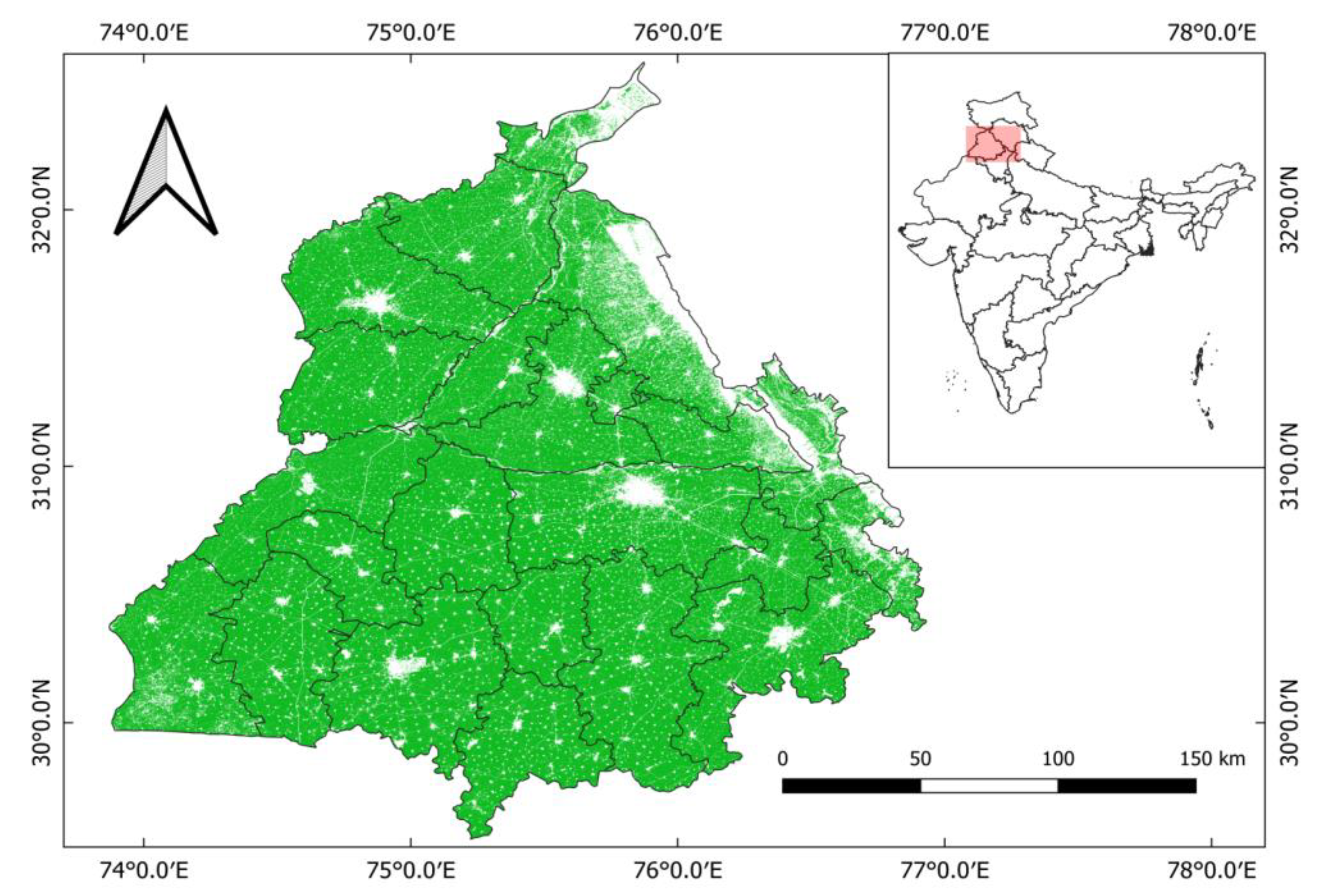
Figure 2.
Workflow for burnt area detection in Punjab.
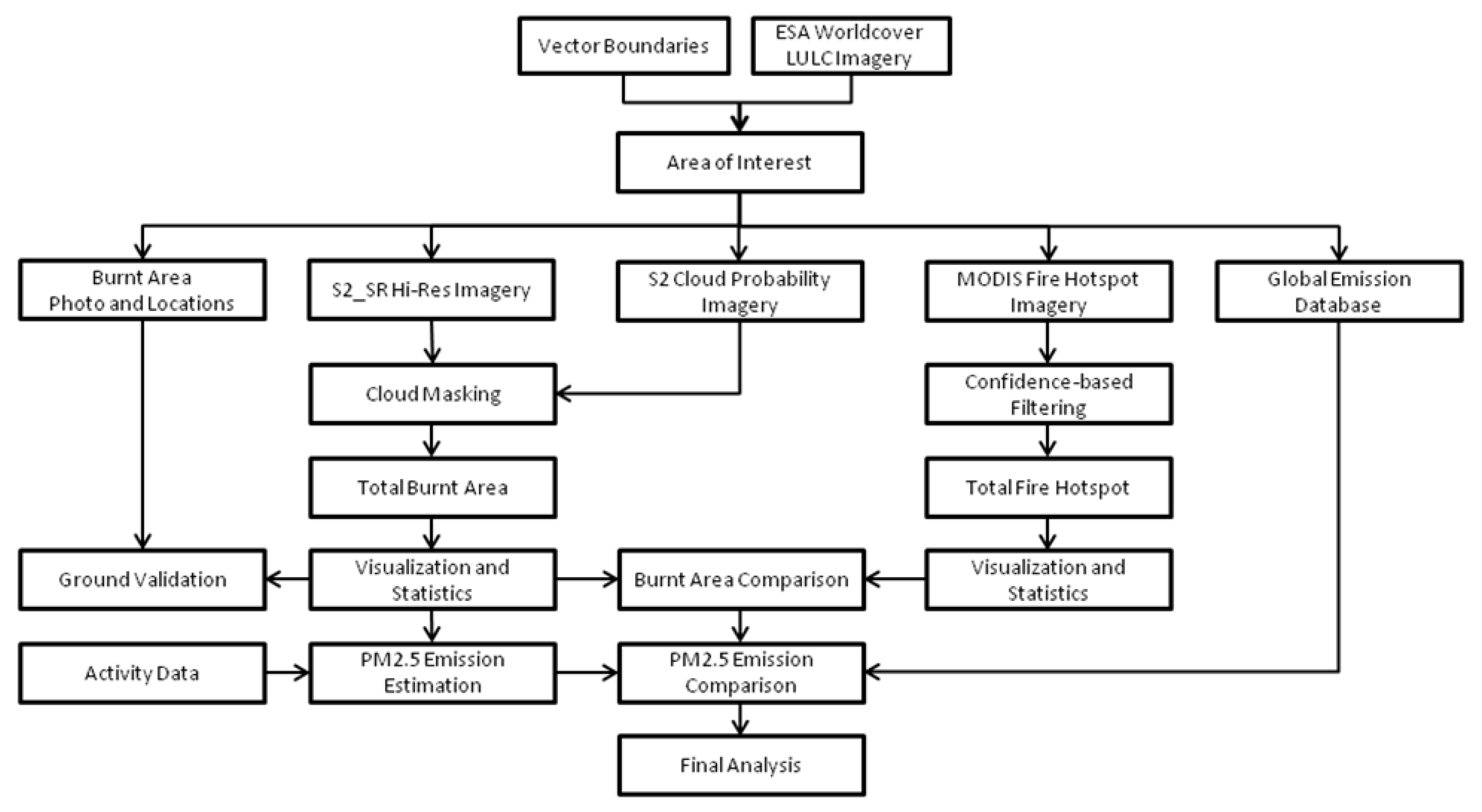
Figure 3.
dNBR histograms across Punjab for multiple time periods during 2022–2024. Each curve represents the frequency of pixels per bin (bin width = 0.04), as computed using consistent bin edges. Histograms are visualized as line graphs for clarity. The vertical black line at a dNBR value of 0.1 represents the threshold used to classify burnt pixels.
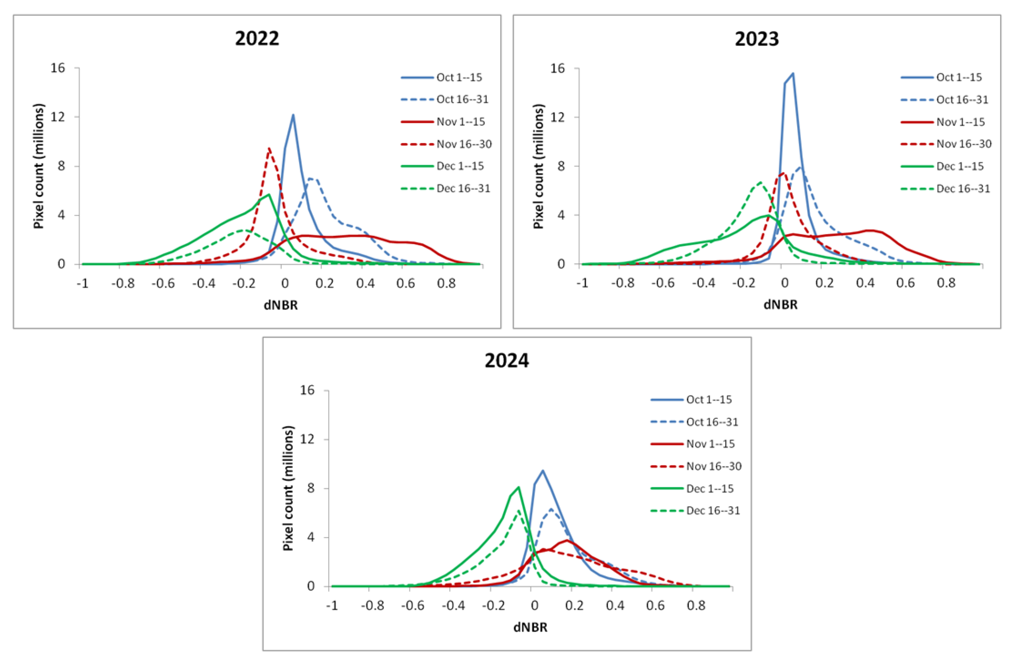
Figure 4.
Burn severity maps of Punjab for October–December from 2022 (a), 2023 (b), and 2024 (c). White areas represent unburnt regions, non-cropland areas, and regions omitted because of cloud masking.
Figure 4.
Burn severity maps of Punjab for October–December from 2022 (a), 2023 (b), and 2024 (c). White areas represent unburnt regions, non-cropland areas, and regions omitted because of cloud masking.
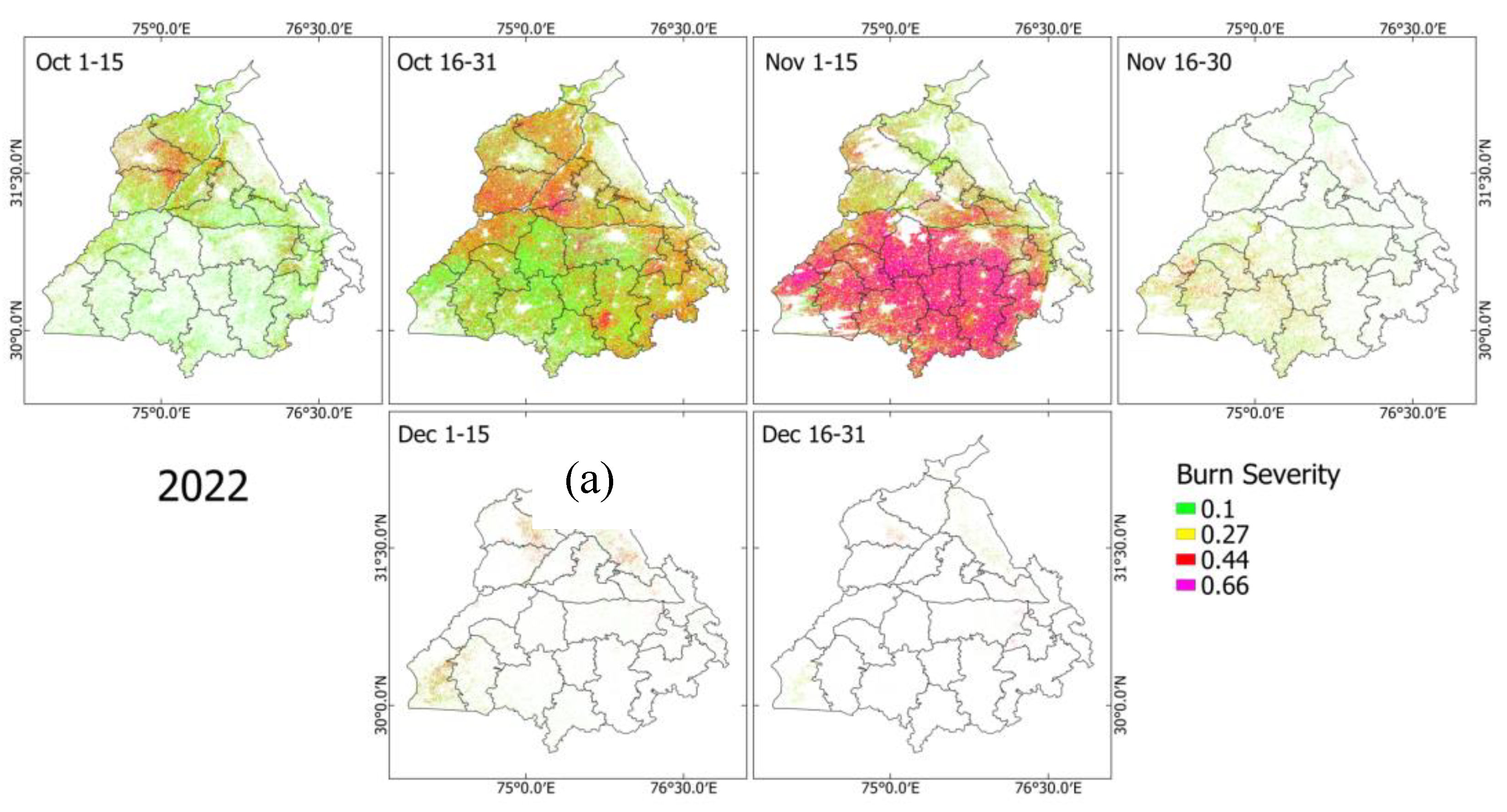

Figure 4.
continued from previous page.
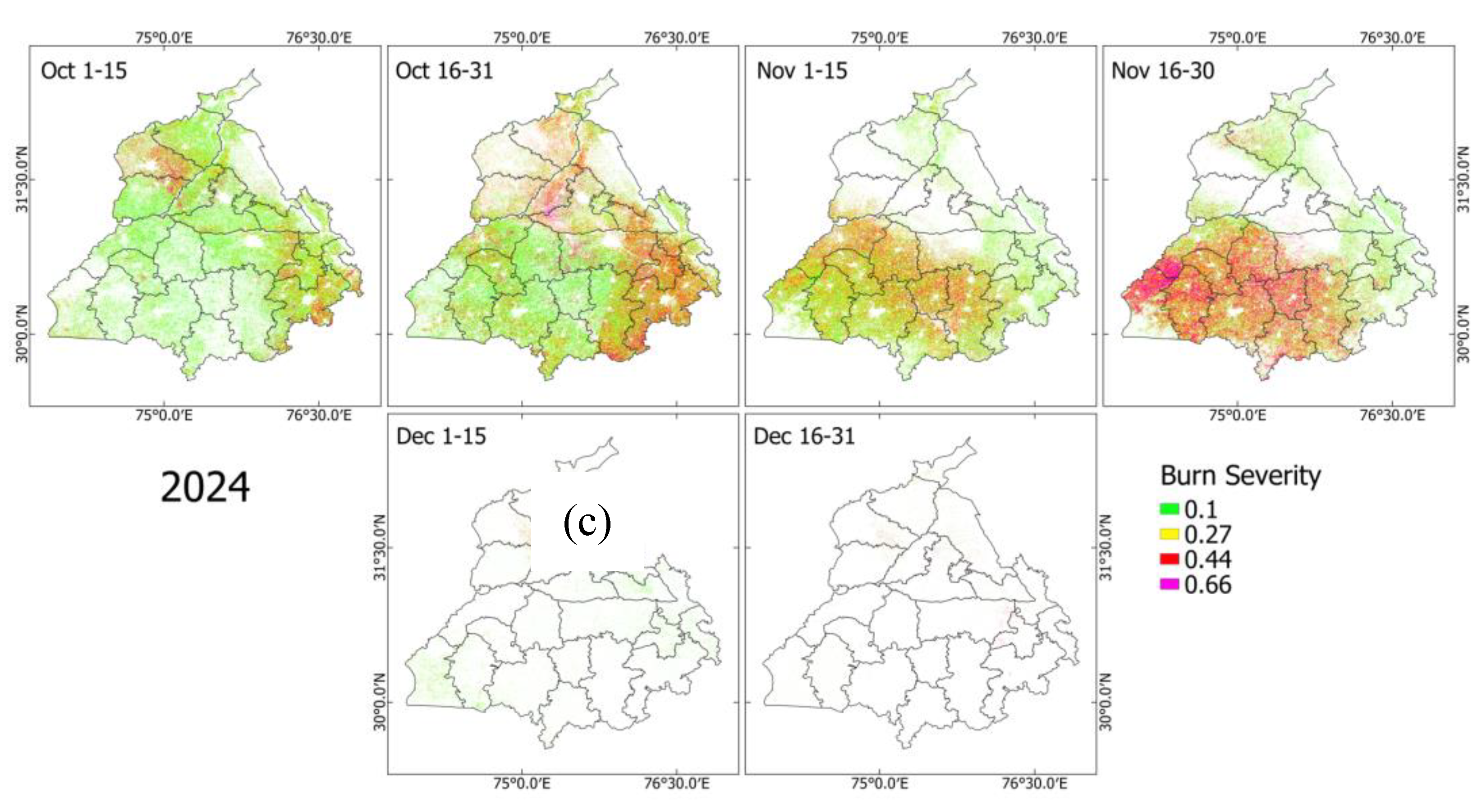
Figure 5.
Total burnt areas (BA), shown as colored bar charts, and mean burn severity (dNBR), shown as colored dashed lines, across Punjab during October–December in 2022–2024.
Figure 5.
Total burnt areas (BA), shown as colored bar charts, and mean burn severity (dNBR), shown as colored dashed lines, across Punjab during October–December in 2022–2024.
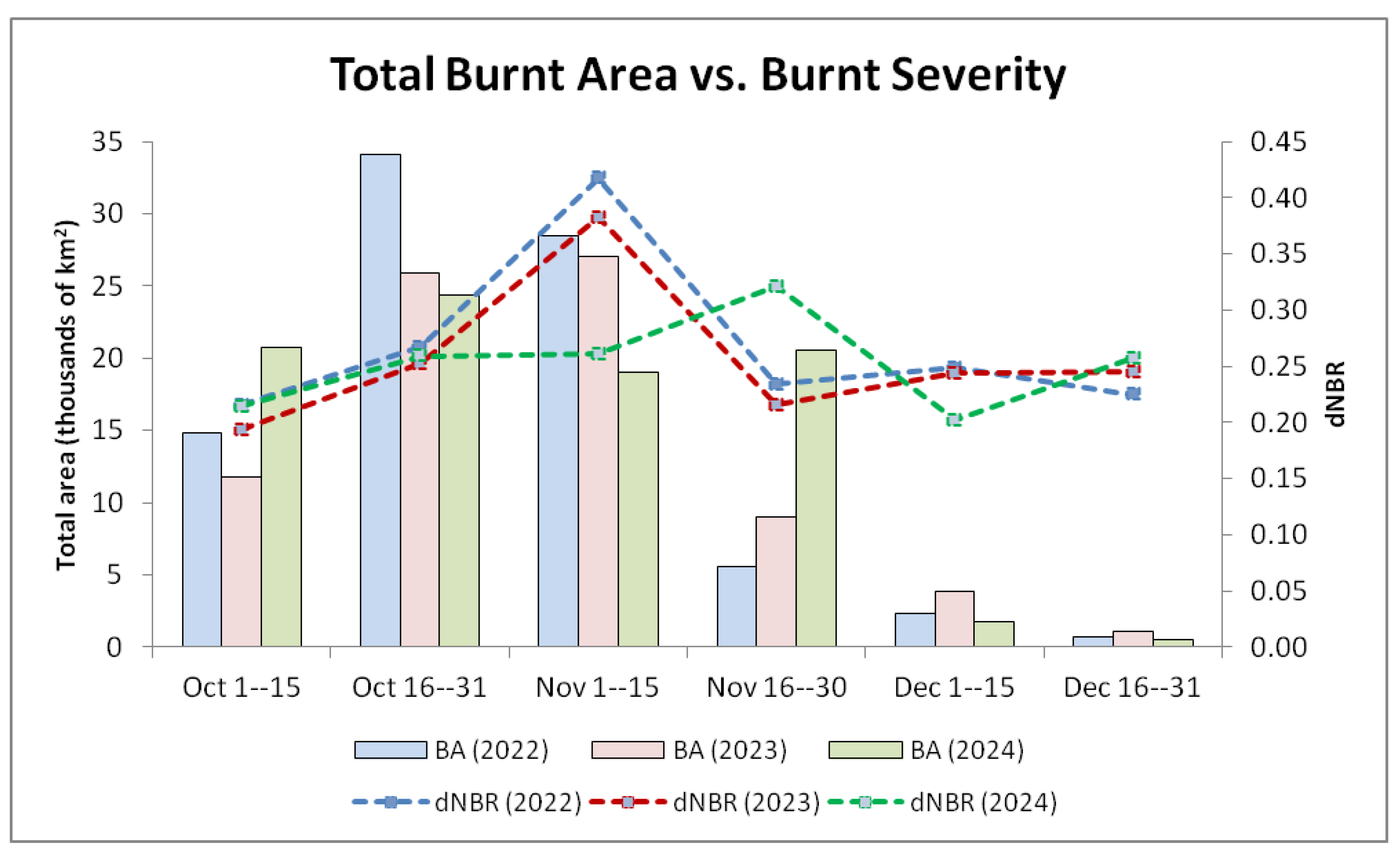
Figure 6.
Ground photographs of post-fire fields at two locations in Ludhiana, Punjab, taken on October 30, 2022 (A1) and November 6, 2022 (B1). BA maps of the corresponding area are presented in the bottom panels (A2 and B2, respectively) with each exact location denoted as a black circle. The burn severity value of each location is shown at the bottom left corner of the BA maps. White areas in BA maps represent unburnt regions, non-cropland areas, and regions omitted because of cloud masking.
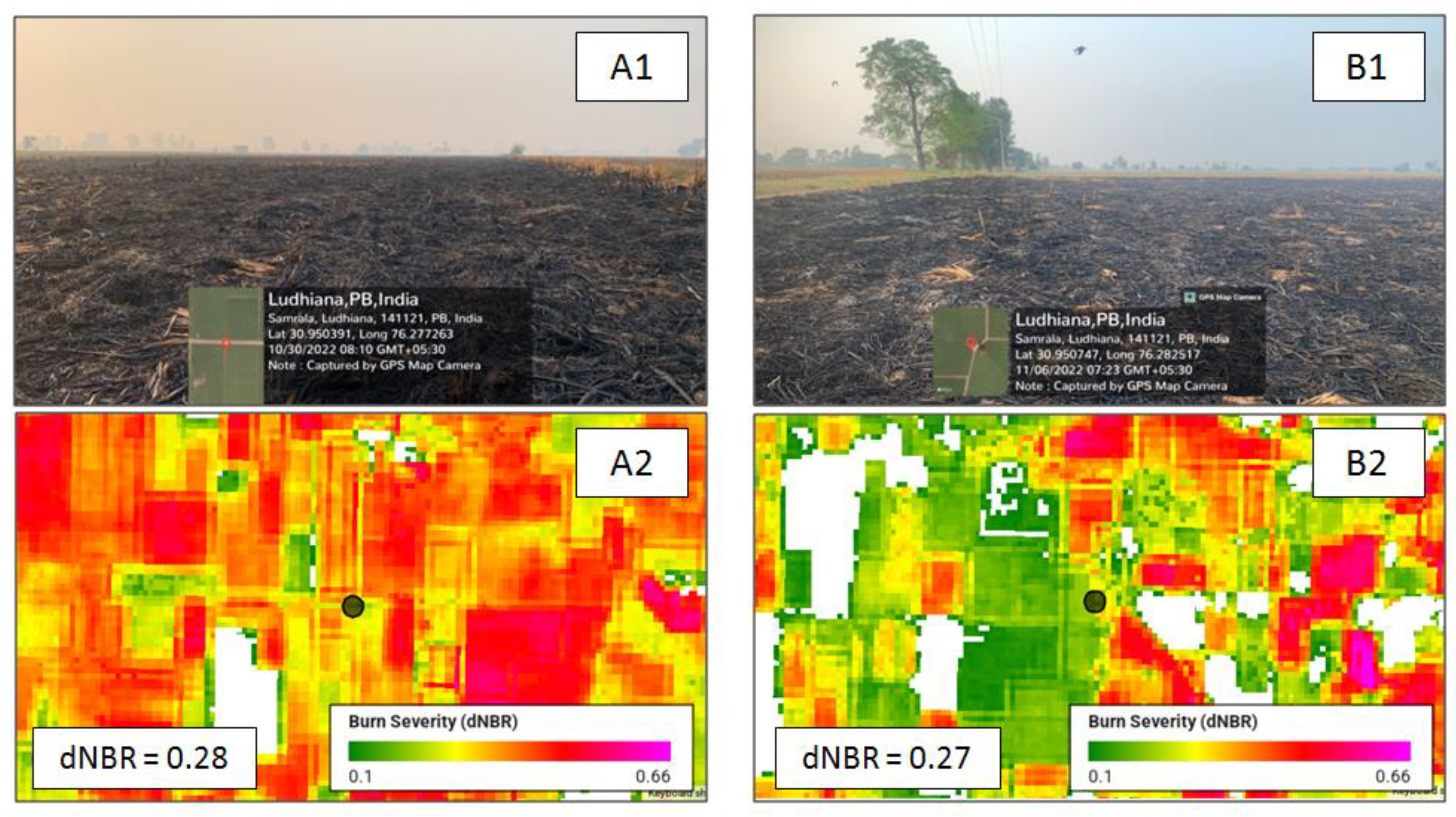
Figure 7.
Burnt areas (BA) detected by Sentinel-2 Surface Reflectance (S2 SR) (columns 1 and 2) and MODIS (columns 3 and 4) in 2022. Each row represents a different month of observation, with corresponding dates shown at the top-right corner of each map.
Figure 7.
Burnt areas (BA) detected by Sentinel-2 Surface Reflectance (S2 SR) (columns 1 and 2) and MODIS (columns 3 and 4) in 2022. Each row represents a different month of observation, with corresponding dates shown at the top-right corner of each map.
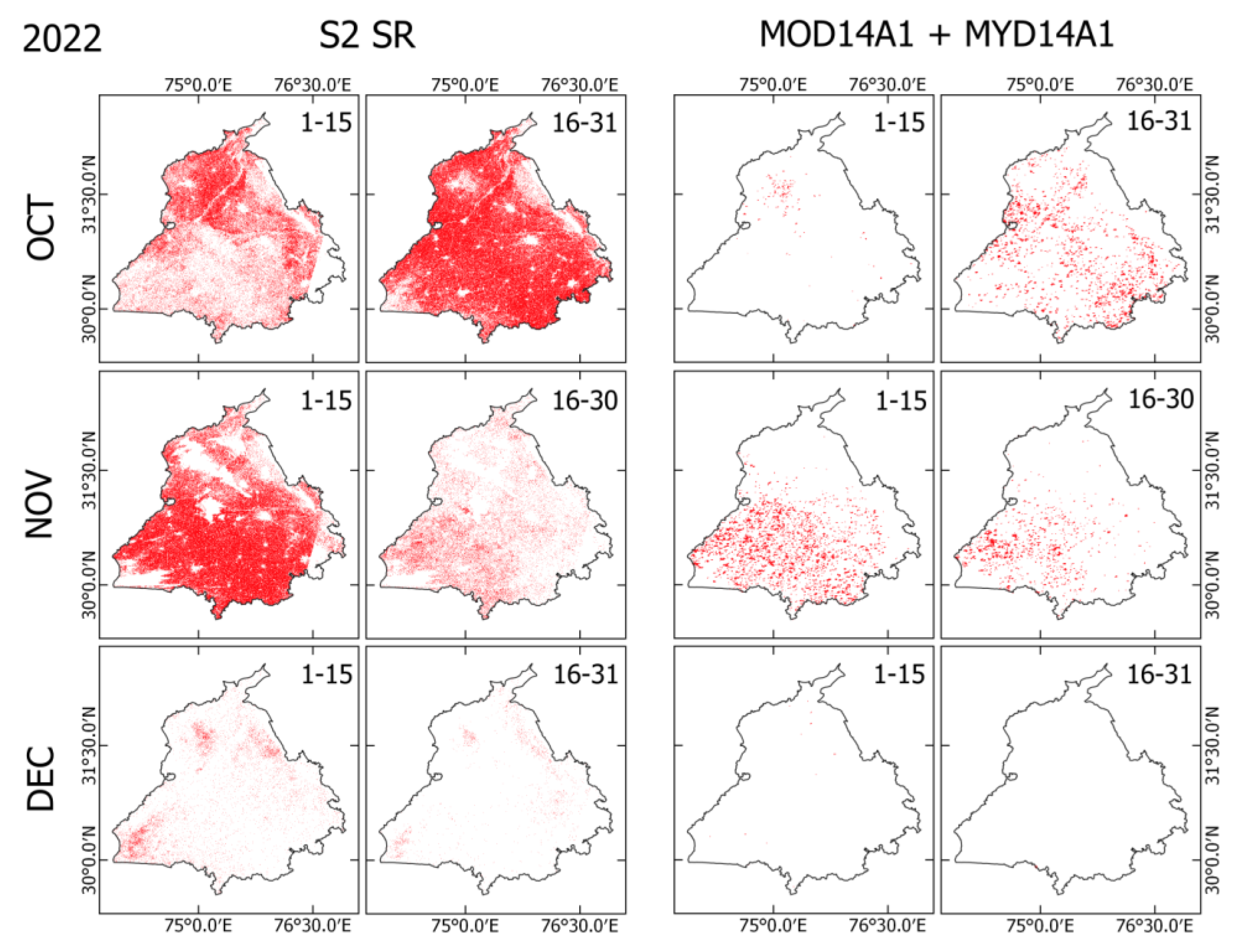
Figure 8.
Burnt areas (BA) detected by Sentinel-2 Surface Reflectance (S2 SR) (columns 1 and 2) and MODIS (columns 3 and 4) in 2023. Each row represents a different month of observation, with corresponding dates shown at the top-right corner of each map.
Figure 8.
Burnt areas (BA) detected by Sentinel-2 Surface Reflectance (S2 SR) (columns 1 and 2) and MODIS (columns 3 and 4) in 2023. Each row represents a different month of observation, with corresponding dates shown at the top-right corner of each map.

Figure 9.
Burnt areas (BA) detected by Sentinel-2 Surface Reflectance (S2 SR) (columns 1 and 2) and MODIS (columns 3 and 4) in 2024. Each row represents a different month of observation, with corresponding dates shown at the top-right corner of each map.
Figure 9.
Burnt areas (BA) detected by Sentinel-2 Surface Reflectance (S2 SR) (columns 1 and 2) and MODIS (columns 3 and 4) in 2024. Each row represents a different month of observation, with corresponding dates shown at the top-right corner of each map.
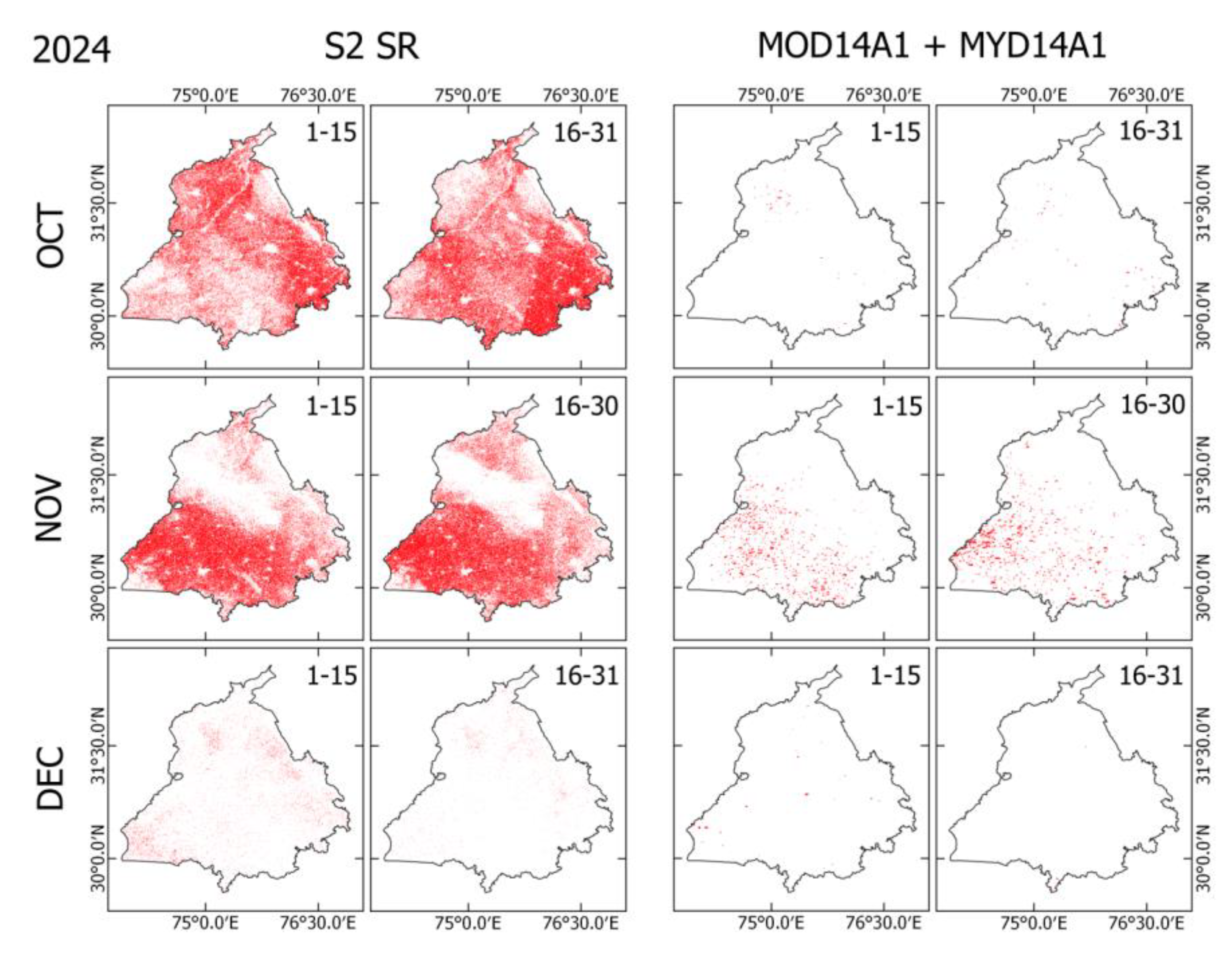
Figure 10.
Total burnt areas (BA) detected by Sentinel-2 Surface Reflectance (S2 SR) and MODIS during October–December in 2022–2024, shown as colored bar charts. BA percentages of corresponding periods for each sensor are presented as colored dashed lines.
Figure 10.
Total burnt areas (BA) detected by Sentinel-2 Surface Reflectance (S2 SR) and MODIS during October–December in 2022–2024, shown as colored bar charts. BA percentages of corresponding periods for each sensor are presented as colored dashed lines.
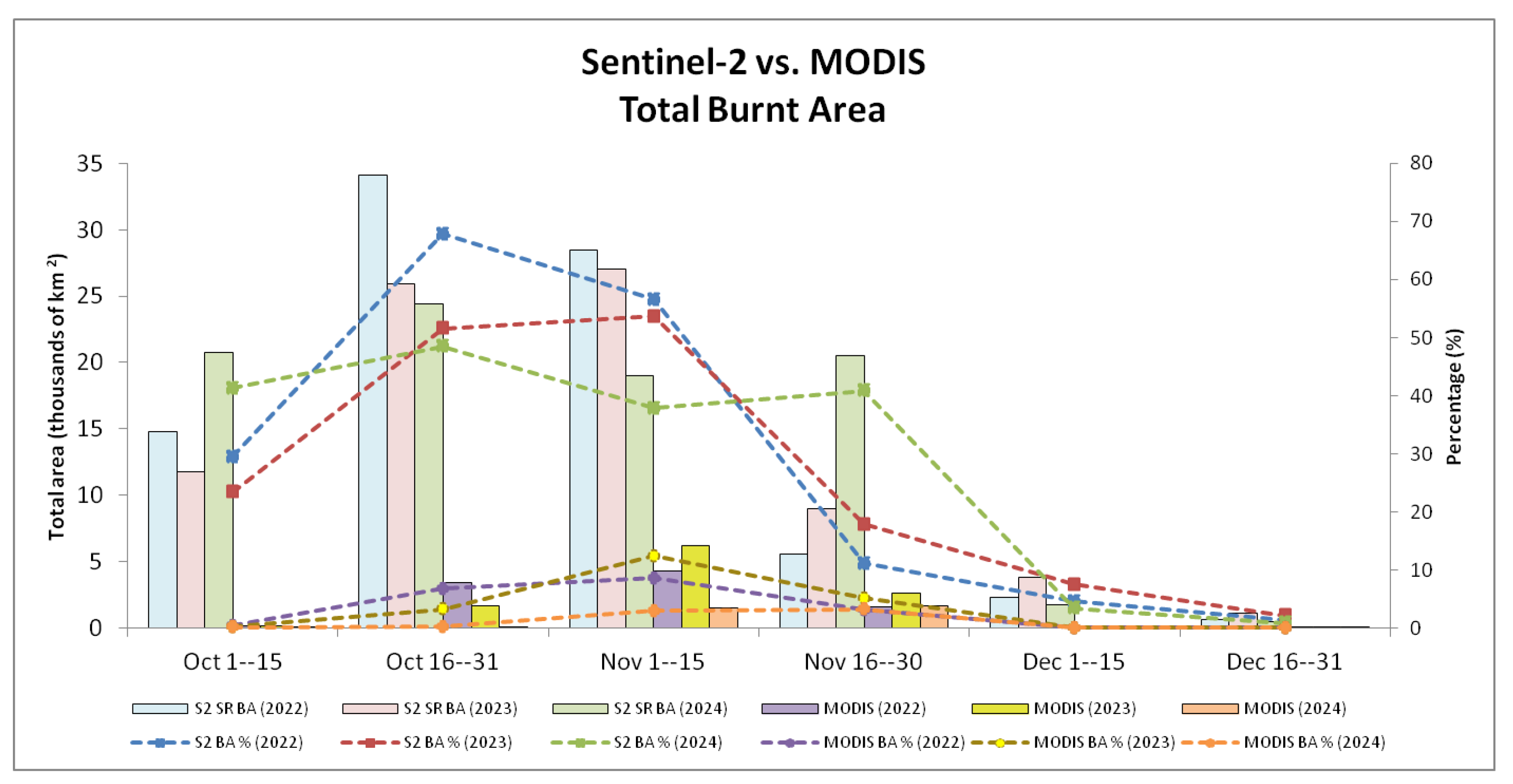
Figure 11.
Chart diagram of PM2.5 emission estimated by Sentinel-2-derived burnt area (BA) compared to EDGARv.8.1 agricultural PM2.5 emission during October–December 2022.
Figure 11.
Chart diagram of PM2.5 emission estimated by Sentinel-2-derived burnt area (BA) compared to EDGARv.8.1 agricultural PM2.5 emission during October–December 2022.
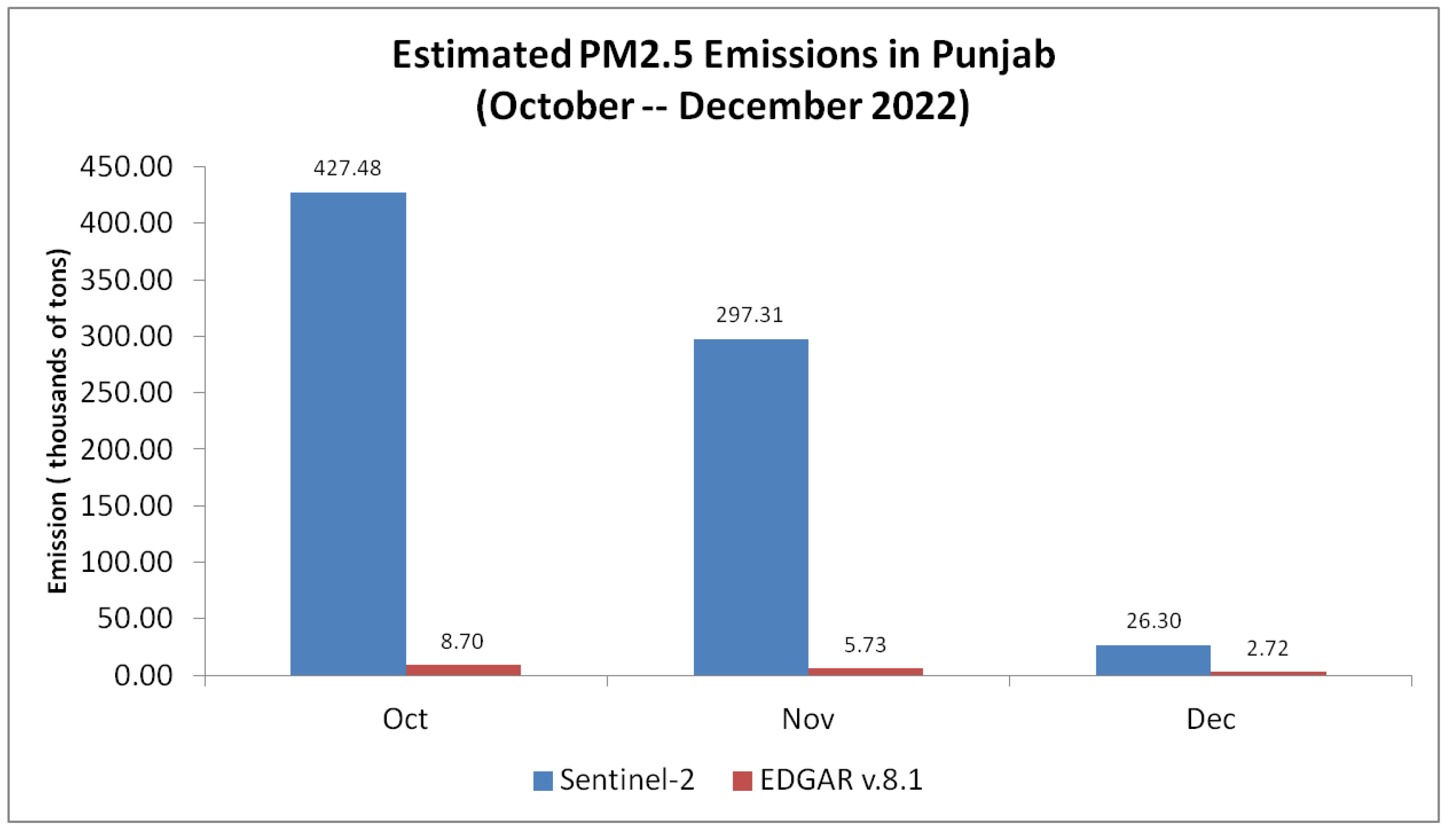

Table 1.
Burn severity values calculated from dNBR.
| Severity Level | dNBR Range (Scaled by 103) |
|---|---|
| Unburnt | Less than 100 |
| Low severity | +100 — +269 |
| Moderate severity (low) | +270 — +439 |
| Moderate severity (high) | +440 — +659 |
| High severity | +660 — +1300 |
Disclaimer/Publisher’s Note: The statements, opinions and data contained in all publications are solely those of the individual author(s) and contributor(s) and not of MDPI and/or the editor(s). MDPI and/or the editor(s) disclaim responsibility for any injury to people or property resulting from any ideas, methods, instructions or products referred to in the content. |
© 2025 by the authors. Licensee MDPI, Basel, Switzerland. This article is an open access article distributed under the terms and conditions of the Creative Commons Attribution (CC BY) license (http://creativecommons.org/licenses/by/4.0/).
Copyright: This open access article is published under a Creative Commons CC BY 4.0 license, which permit the free download, distribution, and reuse, provided that the author and preprint are cited in any reuse.


