Submitted:
09 July 2025
Posted:
10 July 2025
You are already at the latest version
Abstract
Spacecraft imaging of planetary surfaces often suffers from motion-induced blur when the relative velocity between the spacecraft and target is high. We present an automated deblurring framework that derives a one-dimensional point spread function (PSF) directly from the spacecraft’s imaging geometry—without relying on star-field calibration—and applies Wiener deconvolution to restore image sharpness. We validate our method on fourteen sub-meter-per-pixel SRC images of Phobos acquired by Mars Express over four distinct orbits. With an approximately 40-pixel linear PSF and an assumed 16 dB noise level, our pipeline significantly enhances surface feature visibility, enabling fine-scale geological analysis. This technique is readily transferable to other motion-degraded planetary datasets.
Keywords:
Phobos
; Mars Express
; motion blur
; image restoration
; Wiener deconvolution
; point spread function
; spacecraft imagery
; Super Resolution Channel
1. Introduction
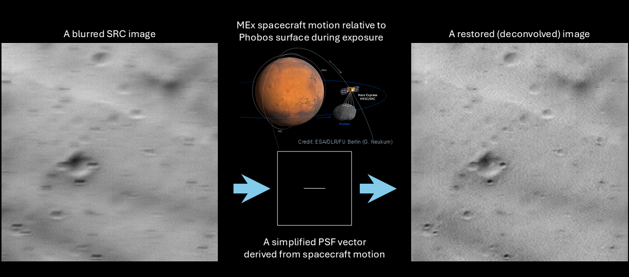
Motion-induced blur (“motion smear”) degrades spacecraft imagery when the relative motion between the sensor and target is substantial, hindering detailed surface characterization. Notable cases include Mars Express’s Super-Resolution Channel (SRC) images of both Phobos [1] and Deimos [2], Viking Orbiter 2’s VIS captures of Deimos [3,4], New Horizons Long Range Reconnaissance Imager (LORRI) images of Arrokoth [5], and both Rosetta’s NAC and Philae’s ROLIS observations of comet 67P/Churyumov–Gerasimenko [6,7]. Although SRC can achieve sub-meter sampling and may offer the highest resolution images currently available for Phobos, residual “pepper” noise and severe smear have limited its scientific exploitation [1,8]. By modeling the blur as a linear PSF determined purely from spacecraft ephemeris and exposure timing, and applying Wiener filtering, we deliver a reproducible, one-shot deconvolution workflow that restores sub-meter detail across diverse imaging conditions.
2. Materials and Methods
2.1. Dataset Selection and Pre-Processing
As the spacecraft approaches a target body, the resulting images would become both more blurred and higher in resolution. Thus, using the European Space Agency (ESA) Planetary Science Archive (PSA) web interface, we first listed Mars Express High Resolution Stereo Camera (HRSC) [9] Super Resolution Channel (SRC) level 3 data products that were obtained with a slant distance of less than 300 km to Phobos. We browsed all publicly accessible datasets acquired within observation dates since 2003 to the latest release (as of June 2025). After that, we manually selected SRC image IDs whose boresight intersects visible (not dark) surfaces of Phobos by visual inspection. This finally achieved a list of fourteen highest-resolution (better than a few meters per pixel) SRC images which were observed during orbits 5851 (23 July 2008), orbit 7926 (10 March 2010), orbit 8974 (9 January 2011), and orbit 14776 (26 August 2015) (Table 1), three of which are consistent with those listed by Witasse, et al. [10].
Based on that, we acquired Planetary Data System (PDS) IMG data sets of HRSC radiometric Reduced Data Record (RDR) Extension series (EXT2, EXT3, EXT5, and EXT7) Version 4.0 [11,12,13,14] from the PDS Geosciences Node server (https://pds-geosciences.wustl.edu/mex). Also, we downloaded the MEx-related Spacecraft, Planet, Instrument, C-matrix, Events (SPICE) kernels [15] by running the Integrated Software for Imagers and Spectrometers (ISIS) version 8.3.0 developed by United States Geological Survey (USGS) [16], as well as an extra SPK kernel, MEX_STRUCT_V01.BSP, from the SPICE datasets in the ESA PSA server (MEX-E-M-SPICE-6-V2.0) [17].
We first converted their PDS IMG files to ISIS cubes, and attached MEx SPICE kernels to the cubes by running both "hrsc2isis" and "spiceinit" commands of ISIS 8.3.0 (Figure 1). To obtain better shift of surface intercept points to be required in the following image restoration, during "spiceinit", we add MEX_STRUCT_V01.BSP as an extra kernel and the latest, finest (~18-m mean spacing) shape model [8] as a DSK kernel that was converted from phobos_g_018m_spc_0000n00000_v002.obj (available at https://sbmt.jhuapl.edu/shared-files/) by using the Navigation and Ancillary Information Facility (NAIF) SPICE utility program MKDSK (https://naif.jpl.nasa.gov/pub/naif/toolkit_docs/C/ug/mkdsk.html).
2.2. Denoising
The MEx SRC level 3 data products are already calibrated as the MEx team has officially reduced most of the pepper (dark) noise left in the level 2 products. However, a few pepper pixels still remain in the level 3 products. We regarded these residual pepper pixels as NULL pixels using the ISIS ”specpix”, which would cause problematic errors when subsequent processing in frequency-domain. Also, each PDS label contains the parameter "LINE_FIRST_PIXEL = 3", which is intended to indicate that the first two lines do not contain valid data. However, this assumption does not always hold because several of the individual cubes have data lines within the first three lines. Thus, we marked the pixels having DNs less than 200 within the first three lines as Low Representation Saturation (LRS), and completely removed them as well as dark pixels (75 NULL pixels per cube) by replacing the mean of their surrounding pixels by running ISIS “noisefilter” (third and fourth boxes in Figure 1). We repeated this noise filtering process until no LRS pixels remained in the resulting cube (twice for h5851_0003_sr3 and three times for h5851_0004_sr3). Moreover, any pixel whose raw DN value was ≤ –200 was considered anomalously dark and substituted with the average DN of its eight neighboring pixels. As exemplified in Figure 2, the NULL and dark pixels are removed from all SRC cubes.
2.3. PSF Estimation
The motion-induced blur can be modeled as a one-dimensional linear point spread function (PSF), parameterized by the spacecraft’s instantaneous ground-track velocity and the detector exposure time. These parameters are effectively determined by the spacecraft’s positions in body-fixed coordinate at the start and end of the exposure. Therefore, the resulting PSF’s length and its orientation (along the projected motion vector over Phobos) can be derived directly from spacecraft telemetry.
After collecting values regarding the IMG/cube labels "START_TIME" (UTC1), "STOP_TIME" (UTC2), and "EXPOSURE_DURATION" (exposure) with the USGS Abstraction Layer for Ephemerides (ALE) library [18,19,20], we first performed calculation of “high-accuracy” observation start and stop timings in forms of ephemeris time (ET) with microsecond precisions (ET’1 and ET’2,) based on:
where ET1 and ET2 are the ET expressions of UTC1 and UTC2, respectively.
Conversions from ET to UTC and vice versa were implemented by uses of SpiceyPy et2utc and utc2et, respectively. The resulted UTC′1 and UTC′2 (UTC expressions of the resulted ET’1 and ET’2) about the selected SRC images are listed in Table 2.
For PSF estimation, we started calculating the SRC boresight intersections with the Phobos surface DSK in the Phobos’ body-fixed reference frame “IAU_PHOBOS”. Using SpiceyPy [21] sincpt function with the aberration correction option of “CN+S” (both light time and stellar correction) gives two positional vectors at ET1’ simultaneously: one from observer (obs; the origin of SRC boresight, “MEX_HRSC” whose SPICE body code is -41200) to the surface intercept point (spt) ( in Figure 3) and another from Phobos center (bod) to the same spt ( in Figure 3). Taking their vector difference gives (as shown in Figure 3):
Similarly, using SpiceyPy spkpos function with the “CN+S” aberration correction, we obtain a positional vector at ET2’ from obs to bod ( in Figure 3) as well. Then, using it with the resulted from equation (3), we can calculate the vector directing from obs at ET2’ to obs at ET1’:
Using derived from equation (4) and , we finally gain the positional vector at ET2’ from obs to spt ( in Figure 3):
The two resulting position vectors from obs to spt at ET1’ and ET2’, and , are expressed in the Phobos-body fixed frame “IAU_PHOBOS” (SPICE FK ID: 10021). We thus translated these vectors into the ones in the instrument frame “MEX_HRSC_SRC” (SPICE FK ID: -41220) by multiplying the frame-to-frame (“IAU_PHOBOS” to “MEX_HRSC_SRC”) transformation matrices at ET1’ and ET2’ that were generated by SpiceyPy function pxform. Using two obs-to-spt vectors expressed in the “MEX_HRSC_SRC” frame, we derived image coordinates of the two corresponding points on the SRC image plane:
where (X1, Y1) and (X2, Y2) are respectively the coordinates of the projected point at ET1’ and ET2’, (x1, y1, z1) and (x2, y2, z2) are respectively the components of and expressed in the “MEX_HRSC_SRC” frame; focal length is 9.8476e+5 μm (= 984.76 mm [22]), pixel sizex is 9.0 μm/pixel, and pixel sizey is 9.0 μm/pixel [9], each of which is stored in SPICE IK MEX_HRSC_V09.TI.
Finally, we obtained the shift of the projected points during exposure on the SRC image plane by calculating their differences:
The obtained PSF geometries are summarized in Table 3. By using longer exposures—values matching the SRC observation durations—our pipeline extracted extended PSFs, which is consistent with the initial expectation of this study. Most of the vertical components of the shifts are close to zero relative to horizontal components, so that the resulting PSF can be approximated to be a horizontally flat line (See Figure 4 for a typical case).
2.4. Wiener Deconvolution
There are two major deconvolution methods to restore degraded images: Wiener deconvolution [23] and Lucy–Richardson (or Richardson–Lucy) deconvolution [24,25]. Wiener deconvolution uses a linear, closed-form filter in the frequency domain, which has achieved restoration of planetary images, such as the Near Earth Asteroid Rendezvous (NEAR) Shoemaker spacecraft Multispectral Imager (MSI) images of asteroid Eros [26,27].
Wiener algorithm computes a single “optimal” filter that, when applied to the blurred image’s Fourier transform , yields an estimate of the true image’s transform :
where are the frequency coordinates corresponding to the spatial coordinates , (and hence ) is the transfer function (Fourier-domain PSF), is complex conjugate of , and are the noise and signal power spectra, respectively (that is, is the noise-to-signal power ratio), Signal-to-Noise Ratio (SNR)?a dimensionless quantity?is given by , and is the estimate of the true image’s Fourier spectrum.
Lucy–Richardson deconvolution uses an iterative, non-linear algorithm in the spatial domain, and has been applied to planetary images, including MEx/SRC images of Phobos [28] and Mars [22] (but not so high resolution and terribly blurred as those addressed in this study). Lucy–Richardson deconvolution is based on maximum-likelihood estimation assuming Poisson (photon) noise. Starting from an initial guess , it refines via
where “∗” denotes convolution and h is the PSF reversed. Each pass sharpens details and suppresses noise according to the Poisson likelihood.
Either would work for restoring SRC images; however, we selected Wiener deconvolution for the restoration in this study. This is because the PSF can be computed a priori from precise motion and exposure data, the closed-form Wiener filter offers a direct, non-iterative solution that (i) fully exploits the known kernel, (ii) minimizes noise amplification via the noise term, and (iii) avoids iteration-dependent artifacts and convergence issues associated with Lucy–Richardson (Table 4). Therefore, we used Wiener deconvolution, using with the linear PSFs aforementioned and an empirically determined SNR = 16 dB (i.e., in linear scale) that works well regardless of a variety of SRC observation conditions. To mitigate serious ringing artifacts of output boundaries after deconvolution [29], we also used edge tapering algorithm (Gaussian-weighted taper at the edges) with the width of 81 pixels on both right- and left-sides (and no tapering at top and bottom sides) of each input image beforehand.
Although MATLAB offers built-in routines for Wiener deconvolution and edge tapering (e.g., deconvwnr and edgetaper), we chose to avoid reliance on proprietary software by reimplementing these methods in OpenCV. Specifically, we extended OpenCV’s deconvolution sample (https://github.com/opencv/opencv/blob/master/samples/python/deconvolution.py) to include edge tapering, yielding a fully open-source solution. Our Python implementation will be made available at https://github.com/ryodohemmi/public upon publication.
3. Results
We successfully restored motion-blurred SRC images of the four MEx orbits, significantly reducing blur and enhancing geological feature visibility. Our pipeline establishes a robust and objective framework for future restoration and analysis of motion-blurred planetary imagery.
3.1. Orbit 5851
Within the four selected MEx orbits (and most of all MEx orbits), the orbit 5851 has observed SRC images with the second highest resolutions (~0.86 m/pixel; Table 1) and the shortest exposure duration (~14 milliseconds; Table 2), which caused severe motion blurs with lengths of ~44 pixels (Table 3) in resulting images. However, unclear surface features, such as impact craters and portions of lineaments, have appeared unequivocally after restoration, as shown in Figure 5. Noisy artifacts in images are still visible, but ringing artifacts at edges are minimized in restored images. As for small-scale craters, a diversity of their depths, rims, floors, and degradational states is also identifiable, which is consistent with morphologies of sub-kilometer-scale craters on Phobos [30]. Based on the above inspection, we conclude that our restoration pipeline restored the SRC images in orbit 5851 to a satisfying level of quality.
3.2. Orbit 7926
The SRC image of MEx orbit 7926 has the lowest resolution and the longest slant distance (~2.7 m/pixel and ~292 km; Table 1) among all the SRC images selected in this study. With an exposure duration as short as that of orbit 5851, the shortest PSF only~11 pixels in length (Table 3) caused a slight motion smear to the original image, which is consistent with its appearance in Figure 6a. After our restoration process, we obtained the image that exhibits the well-defined craters and grooves on Phobos. Although the imaging distance to the surface would be proximal on the left side and distal to the right side of the figure, the restoration appears successful on both sides. A few noises are identified on the resulting image; however, the edge tapering effect has not reduced the original image’s quality seriously. As a result, we determined the SRC image of the orbit 7926 was successfully restored.
3.3. Orbit 8974
Seven images acquired in the MEx orbit 8974 have similar resolutions and slant distances to those of the orbit 5851 and a slightly longer exposure duration (~16.1 milliseconds; Table 2) with their PSF lengths of ~46 pixels (Table 3), which cover the southern hemisphere of anti-Mars surface of Phobos (Table 1). As shown in Figure 7, all SRC images captured a wide range of craters sizes and morphologies, and some of them observed lineaments (Figure 7a) and slopes (Figure 7g), which would be significant for analyses in surface irregularity (e.g., [31]). After the deconvolution, the resultant images show well-defined outlines of surface features much better than those of original images. Furthermore, we can identify several-pixel-scale, positive relief features (most likely boulders; Figure 7d, f) that were difficult to identify from original blurred images. Regardless of diverse landscapes, the deconvolved images show few noises and edge-tapered pixels at negligible levels. We express deblurring the orbit 8974 was quite achieved successfully.
3.1. Orbit 14776
Among the selected (and probably all available) MEx SRC images, those acquired in the MEx orbit 14776 are the worst motion-blurred, due to exposures of ~20 milliseconds (Table 2), the closest distance (~52 km), and the highest resolution (~0.47 meter/pixel ; Table 1), which is the hardest to recover by deconvolution. However, as shown in Figure 8, we performed restoration and acquired the images showing identifiable surface features, such as small impact craters and boulder-like positive reliefs. Even though there are noticeable noises and edge-tapering effects left in the resulting images, given the initial bad imaging conditions, we conclude our efforts made them as restored as possible, from a theoretical viewpoint.
4. Discussion
Our motion-blur restoration pipeline?based on an a priori, geometry-derived linear PSF and Wiener deconvolution?robustly recovers sub-meter Phobos surface details under diverse imaging conditions. By computing the PSF directly from spacecraft ephemeris and exposure data, we bypass the need for star-field references or manual kernel tuning, while the closed-form Wiener filter provides built-in noise regularization and avoids iteration-dependent artifacts. The extracted PSFs ranged from ~11 to ~119 pixels in length (reflecting ground-track speed and slant distance) with negligible vertical components, justifying their one-dimensional horizontal approximation.
In the high-resolution, short-exposure case (orbit 5851; 0.86 m/pixel, 14 milliseconds), deconvolution revealed crater morphologies, rim and floor textures, and linear features that were indiscernible in the raw images (Figure 5). Even at the coarsest resolution (orbit 7926; ~2.7 m/pixel, 14 milliseconds), grooves and crater edges sharpened with minimal ringing, demonstrating the method’s resilience to low SNR and large slant distances. For intermediate cases (orbit 8974; ~0.92 m/pixel, 16 milliseconds), deblurred images expose lineaments, slopes, and meter-scale boulders consistent with known Phobos morphologies. Even the most challenging dataset (orbit 14776; 0.47 m/pixel, 20 milliseconds) yielded clear views of small impact craters and positive reliefs, pushing the theoretical restoration limit under severe motion smear.
Compared to spatial-domain, iterative approaches like Lucy–Richardson?which have been applied to SRC and other planetary imagery [22]?our frequency-domain Wiener deconvolution delivers a one-shot solution with explicit control over the noise–sharpness trade-off and guaranteed convergence. Because the PSF is derived from precise SPICE kernels and shape models, our framework is completely reproducible and readily adaptable to other spacecraft instruments suffering motion-induced blur.
Scientifically, recovering sub-meter features enables improved crater counting, regolith maturity analysis, and the generation of high-fidelity digital elevation models on Phobos. This approach can be extended to data from missions with similar blur challenges, and will be especially valuable for the forthcoming MMX mission [32,33]. Integrating our deblurring pipeline into photogrammetric and stereophotoclinometry workflows promises significant gains in topographic precision and geological interpretation.
Nevertheless, our treatment assumes a spatially invariant, linear PSF dominated by along-track motion. In reality, additional blur may arise from cross-track jitter, optical aberrations, or attitude fluctuations. We also adopted a fixed SNR of 16 dB; future work should explore adaptive noise estimation to further suppress residual artifacts. Extending the model to 2D, spatially varying PSFs, and hybridizing Wiener with iterative methods may yield further improvements. Finally, automating noise-term selection based on image statistics will enhance applicability across a broader range of planetary datasets.
5. Conclusions
We have demonstrated an end-to-end pipeline for restoring motion-blurred, high-resolution SRC images of Phobos by automatically deriving a linear PSF from SPICE-based geometry and applying Wiener deconvolution with built-in noise regularization. Across fourteen images spanning four orbits, our method consistently recovers sub-meter surface features and dramatically enhances scientific usability (e.g., elucidating the origins and evolutionary history of small-scale structures and their association with spectral units [34,35]). Notably, this includes the restoration of the highest-resolution SRC images of Phobos acquired to date, which had previously been severely blurred. This approach is fully reproducible, requires no star-field calibration, and is readily extendable to other planetary missions facing motion-induced blur.
Supplementary Materials
The following supporting information can be downloaded at the website of this paper posted on Preprints.org. Data S1: ISIS cube inputs, PSFs, and deblurred outputs.
Author Contributions
Conceptualization, R.H. and H.K.; methodology, R.H.; software, R.H.; validation, R.H; formal analysis, R.H.; investigation, R.H.; resources, R.H. and H.K.; data curation, R.H.; writing—original draft preparation, R.H.; writing—review and editing, R.H. and H.K.; visualization, R.H.; supervision, R.H.; project administration, R.H.; funding acquisition, R.H. All authors have read and agreed to the published version of the manuscript.
Funding
This work was supported by JSPS KAKENHI Grant Number 23H00279.
Data Availability Statement
Datasets of the HRSC instrument have been downloaded from the ESA Planetary Science Archive (https://psa.esa.int) [36]. PDS IMG datasets of SRC level3 products were available at https://pds-geosciences.wustl.edu/mex. We acquired MEx SPICE kernels via ISIS data server and additional SPK from https://archives.esac.esa.int/psa/ftp/MARS-EXPRESS/SPICE/MEX-E-M-SPICE-6-V2.0 as well as those. The Python codes used to denoise and deblur an ISIS cube will be available in the author’s repository, https://github.com/ryodohemmi/public.
Acknowledgments
The authors acknowledge the Principal Investigator G. Neukum (Freie Universitaet, Berlin, Germany) of the HRSC instrument onboard the Mars Express mission for providing datasets in the archive.
Conflicts of Interest
The authors declare no conflicts of interest.
Abbreviations
The following abbreviations are used in this manuscript:
| ALE | Abstraction Layer for Ephemerides |
| DN | Digital Number |
| ESA | European Space Agency |
| MEx | Mars Express |
| NAIF | Navigation and Ancillary Information Facility |
| HRSC | High Resolution Stereo Camera |
| ID | Identifier |
| ISIS | Integrated Software for Imagers and Spectrometers |
| PDS | Planetary Data System |
| PSA | Planetary Science Archive |
| PSF | Point Spread Function |
| RDR | Reduced Data Record |
| SNR | Signal-to-Noise Ratio |
| SPICE | Spacecraft, Planet, Instrument, C-matrix, Events |
| SRC | Super Resolution Channel |
| USGS | United States Geological Survey |
References
- Oberst, J.; Schwarz, G.; Behnke, T.; Hoffmann, H.; Matz, K.D.; Flohrer, J.; Hirsch, H.; Roatsch, T.; Scholten, F.; Hauber, E.; et al. The imaging performance of the SRC on Mars Express. Planetary and Space Science 2008, 56, 473–491. [Google Scholar] [CrossRef]
- Pasewaldt, A.; Oberst, J.; Willner, K.; Wählisch, M.; Hoffmann, H.; Matz, K.D.; Roatsch, T.; Hussmann, H.; Lupovka, V. New astrometric observations of Deimos with the SRC on Mars Express. A&A 2012, 545. [Google Scholar] [CrossRef]
- Veverka, J. The surfaces of Phobos and Deimos. Vistas in Astronomy 1978, 22, 163–192. [Google Scholar] [CrossRef]
- Thomas, P. Surface features of Phobos and Deimos. Icarus 1979, 40, 223–243. [Google Scholar] [CrossRef]
- Spencer, J.R.; Stern, S.A.; Moore, J.M.; Weaver, H.A.; Singer, K.N.; Olkin, C.B.; Verbiscer, A.J.; McKinnon, W.B.; Parker, J.W.; Beyer, R.A.; et al. The geology and geophysics of Kuiper Belt object (486958) Arrokoth. Science 2020, 367, eaay3999. [Google Scholar] [CrossRef]
- Keller, H.U.; Barbieri, C.; Lamy, P.; Rickman, H.; Rodrigo, R.; Wenzel, K.P.; Sierks, H.; A’Hearn, M.F.; Angrilli, F.; Angulo, M.; et al. OSIRIS – The Scientific Camera System Onboard Rosetta. Space Science Reviews 2007, 128, 433–506. [Google Scholar] [CrossRef]
- Schröder, S.E.; Mottola, S.; Arnold, G.; Grothues, H.G.; Jaumann, R.; Keller, H.U.; Michaelis, H.; Bibring, J.P.; Pelivan, I.; Koncz, A.; et al. Close-up images of the final Philae landing site on comet 67P/Churyumov-Gerasimenko acquired by the ROLIS camera. Icarus 2017, 285, 263–274. [Google Scholar] [CrossRef]
- Ernst, C.M.; Daly, R.T.; Gaskell, R.W.; Barnouin, O.S.; Nair, H.; Hyatt, B.A.; Al Asad, M.M.; Hoch, K.K.W. High-resolution shape models of Phobos and Deimos from stereophotoclinometry. Earth, Planets and Space 2023, 75, 103. [Google Scholar] [CrossRef]
- Neukum, G.; Jaumann, R. HRSC: The High Resolution Stereo Camera of Mars Express. In Mars Express: The Scientific Payload; ESA: 2004; Volume SP-1240, pp. 17-35.
- Witasse, O.; Duxbury, T.; Chicarro, A.; Altobelli, N.; Andert, T.; Aronica, A.; Barabash, S.; Bertaux, J.L.; Bibring, J.P.; Cardesin-Moinelo, A.; et al. Mars Express investigations of Phobos and Deimos. Planetary and Space Science 2014, 102, 18–34. [Google Scholar] [CrossRef]
- European Space Agency, R. , Thomas. 'MEX-M-HRSC-3-RDR-EXT2', V4.0. 2022. [Google Scholar] [CrossRef]
- European Space Agency, R. , Thomas. 'MEX-M-HRSC-3-RDR-EXT3', V4.0. 2022. [Google Scholar] [CrossRef]
- European Space Agency, R. , Thomas. 'MEX-M-HRSC-3-RDR-EXT5', V4.0. 2022. [Google Scholar] [CrossRef]
- European Space Agency, R. , Thomas. 'MEX-M-HRSC-3-RDR-EXT7', V4.0. 2022. [Google Scholar] [CrossRef]
- Acton, C.; Bachman, N.; Semenov, B.; Wright, E. A look towards the future in the handling of space science mission geometry. Planetary and Space Science 2018, 150, 9–12. [Google Scholar] [CrossRef]
- USGS-Astrogeology <i>ISIS 8.3.0 Public Release</i>, 8.3. USGS-Astrogeology ISIS 8.3.0 Public Release, 8.3.0; 2024.
- European Space Agency, E.L. , Alfredo. 'MEX-E-M-SPICE-6', V2.0. 2024. [Google Scholar] [CrossRef]
- USGS-Astrogeology <i>Abstraction Layer for Ephemerides (ALE) 0.10.0</i>, 0.10. USGS-Astrogeology Abstraction Layer for Ephemerides (ALE) 0.10.0, 0.10.0; 2024.
- Laura, J.R.; Mapel, J.; Hare, T. Planetary Sensor Models Interoperability Using the Community Sensor Model Specification. Earth and Space Science 2020, 7, e2019EA000713. [Google Scholar] [CrossRef]
- Mapel, J.A.; Berry, K.; Paquette, A.; Rodriguez, K.; Stapleton, S.; Hare, T.M.; Laura, J.R. The Abstraction Layer for Ephemerides Library. In Proceedings of the 4th Planetary Data Workshop, Flagstaff, Arizona; 2019. [Google Scholar]
- Annex, A.M.; Pearson, B.; Seignovert, B.; Carcich, B.T.; Eichhorn, H.; Mapel, J.A.; Von Forstner, J.L.F.; McAuliffe, J.; Del Rio, J.D.; Berry, K.L. SpiceyPy: a Pythonic Wrapper for the SPICE Toolkit. Journal of Open Source Software 2020, 5, 2050. [Google Scholar] [CrossRef]
- Gwinner, K.; Jaumann, R.; Hauber, E.; Hoffmann, H.; Heipke, C.; Oberst, J.; Neukum, G.; Ansan, V.; Bostelmann, J.; Dumke, A.; et al. The High Resolution Stereo Camera (HRSC) of Mars Express and its approach to science analysis and mapping for Mars and its satellites. Planetary and Space Science 2016, 126, 93–138. [Google Scholar] [CrossRef]
- Wiener, N. Extrapolation, Interpolation, and Smoothing of Stationary Time Series: With Engineering Applications; The MIT Press: 1949.
- Richardson, W.H. Bayesian-Based Iterative Method of Image Restoration. J. Opt. Soc. Am. 1972, 62, 55–59. [Google Scholar] [CrossRef]
- Lucy, L.B. An iterative technique for the rectification of observed distributions. The Astronomical Journal 1974, 79, 745–754. [Google Scholar] [CrossRef]
- Li, H.; Robinson, M.S.; Murchie, S. Preliminary Remediation of Scattered Light in NEAR MSI Images. Icarus 2002, 155, 244–252. [Google Scholar] [CrossRef]
- Golish, D.R.; DellaGiustina, D.N.; Becker, K.J.; Bennett, C.A.; Robinson, M.; Crombie, M.K. Blur remediation in NEAR MSI images. Icarus 2023, 400, 115536. [Google Scholar] [CrossRef]
- Pasewaldt, A.; Oberst, J.; Willner, K.; Beisembin, B.; Hoffmann, H.; Matz, K.D.; Roatsch, T.; Michael, G.; Cardesín-Moinelo, A.; Zubarev, A.E. Astrometric observations of Phobos with the SRC on Mars Express. A&A 2015, 580. [Google Scholar] [CrossRef]
- Liu, R.; Jia, J. Reducing boundary artifacts in image deconvolution. In Proceedings of the 15th IEEE International Conference on Image Processing, New York, 2008, 12-15 Oct. 2008; pp. 505–508. [Google Scholar]
- Hemmi, R.; Miyamoto, H. Morphology and Morphometry of Sub-kilometer Craters on the Nearside of Phobos and Implications for Regolith Properties. Transactions of the Japan Society for Aeronautical and Space Sciences 2020, 63, 124–131. [Google Scholar] [CrossRef]
- Takemura, T.; Miyamoto, H.; Hemmi, R.; Niihara, T.; Michel, P. Small-scale topographic irregularities on Phobos: image and numerical analyses for MMX mission. Earth, Planets and Space 2021, 73, 213. [Google Scholar] [CrossRef]
- Kuramoto, K.; Kawakatsu, Y.; Fujimoto, M.; Araya, A.; Barucci, M.A.; Genda, H.; Hirata, N.; Ikeda, H.; Imamura, T.; Helbert, J.; et al. Martian moons exploration MMX: sample return mission to Phobos elucidating formation processes of habitable planets. Earth, Planets and Space 2022, 74, 12. [Google Scholar] [CrossRef]
- Kameda, S.; Ozaki, M.; Enya, K.; Fuse, R.; Kouyama, T.; Sakatani, N.; Suzuki, H.; Osada, N.; Kato, H.; Miyamoto, H.; et al. Design of telescopic nadir imager for geomorphology (TENGOO) and observation of surface reflectance by optical chromatic imager (OROCHI) for the Martian Moons Exploration (MMX). Earth, Planets and Space 2021, 73, 218. [Google Scholar] [CrossRef]
- Kikuchi, H. Simulating re-impacts from craters at the deepest location of Phobos to generate its blue spectral units. Icarus 2021, 354, 113997. [Google Scholar] [CrossRef]
- Kuramoto, K. Origin of Phobos and Deimos Awaiting Direct Exploration. Annual Review of Earth and Planetary Sciences 2024, 52, 495–519. [Google Scholar] [CrossRef]
- Besse, S.; Vallat, C.; Barthelemy, M.; Coia, D.; Costa, M.; De Marchi, G.; Fraga, D.; Grotheer, E.; Heather, D.; Lim, T.; et al. ESA's Planetary Science Archive: Preserve and present reliable scientific data sets. Planetary and Space Science 2018, 150, 131–140. [Google Scholar] [CrossRef]
Figure 1.
Workflow of the whole pipeline of our SRC image deblurring processing.
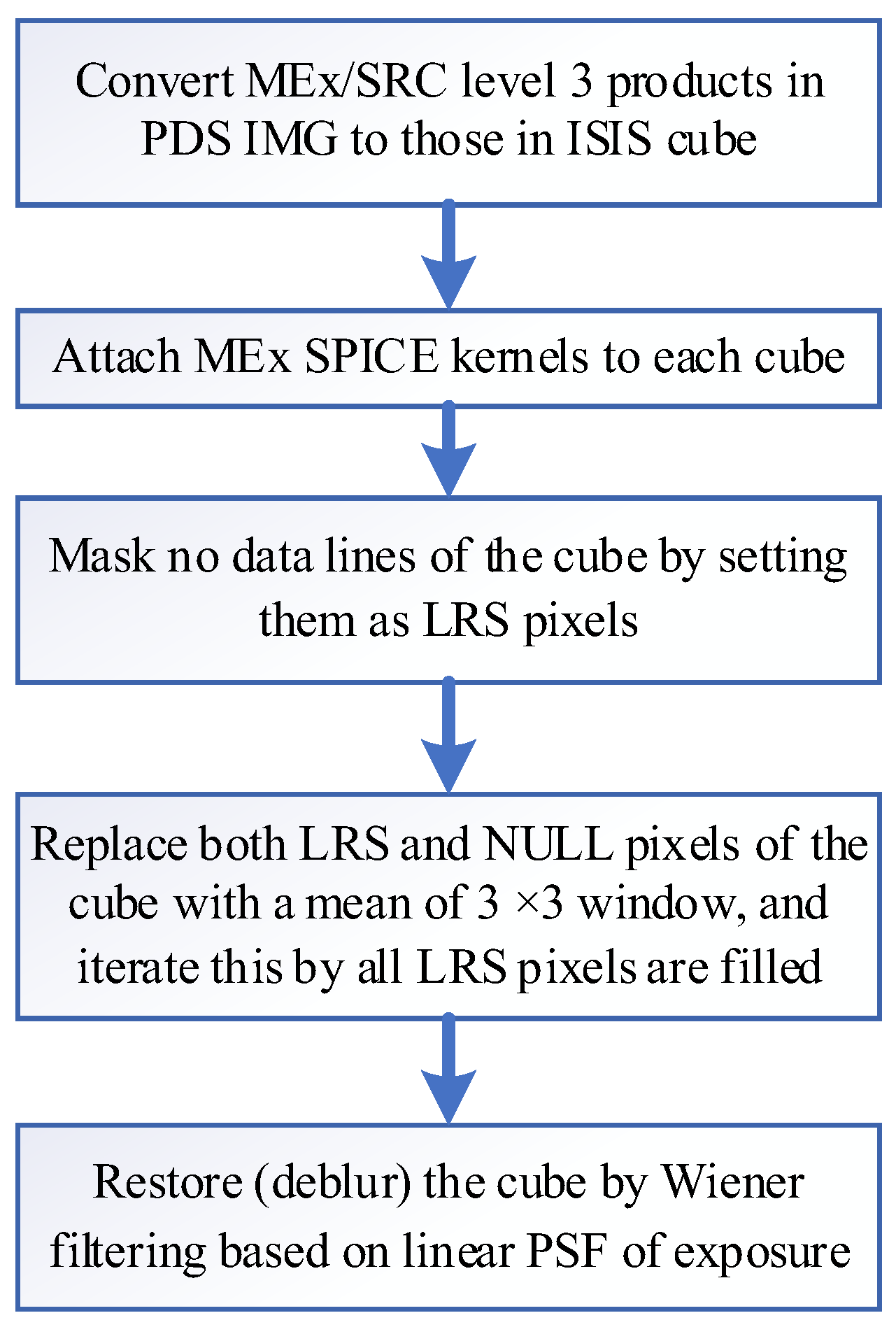
Figure 2.
An SRC image example (a) before and (b) after denoising processing. Red pixels in the panel (a) represent the pepper pixels having NULL values (DN = −1; A close-up view of a digitized PDF version is recommended for readers). The first two dark lines of LRS pixels in (a) are also cleaned after this processing (see panel b). For comparison with the pre-processed image in (a), the denoised image in (b) is shown in a range from 0 to +1195, while its actual range is from +334 to +1195. The SRC image ID is h5851_0003_sr3.
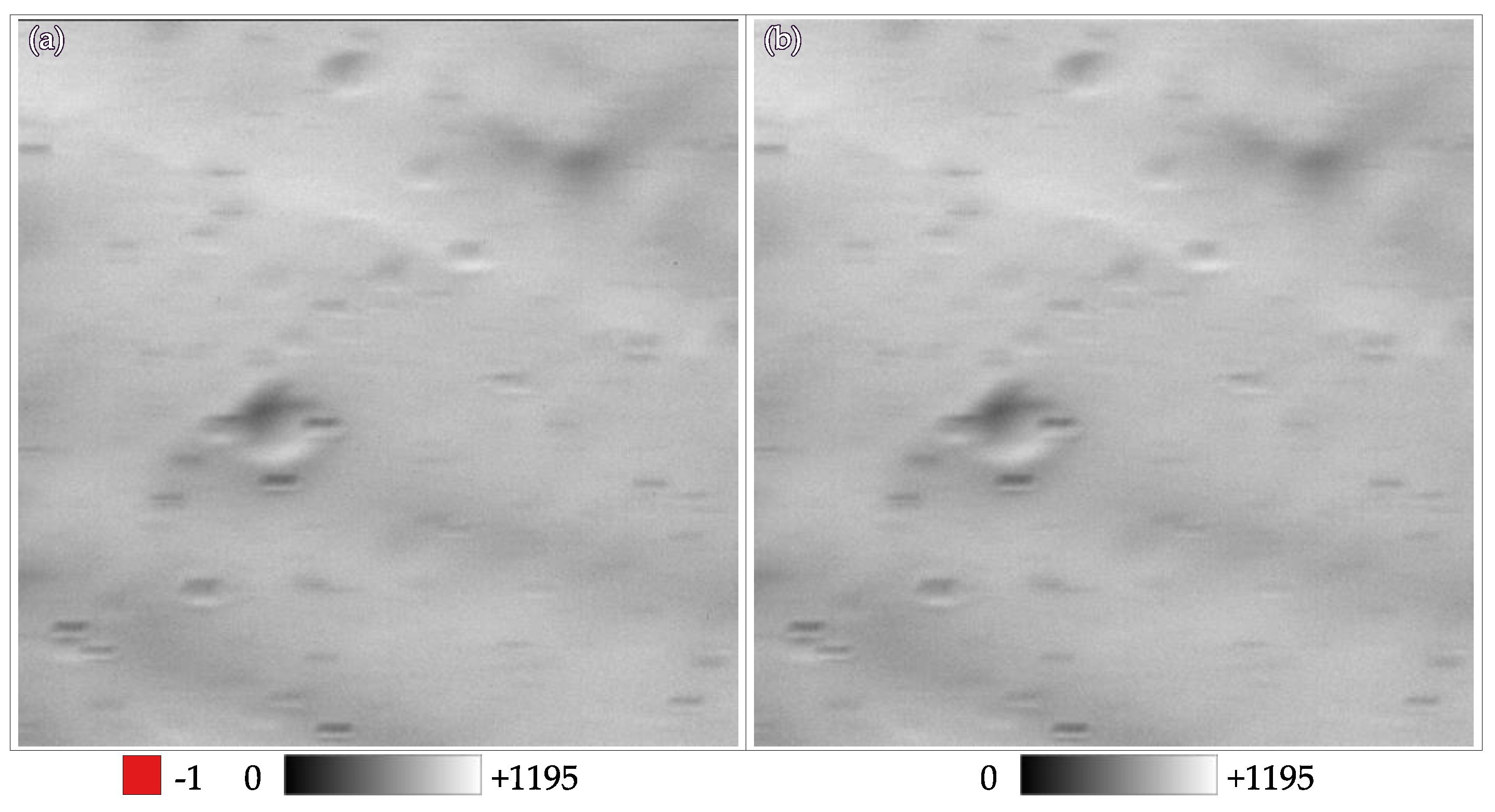
Figure 3.
Schematic illustration of the SRC onboard the MEx spacecraft (S/C) in motion from its side view (top) and the resulting view of the SRC image plane (bottom) during the same SRC exposure duration. (top) Two red arrows show vectors from observer (obs; SPICE name: "MEX_HRSC") to the same surface intercept point (spt) in the IAU_PHOBOS frame. The left and right sides show the observation start time (t1 = ET1′, or UTC1′) and stop time (right side: t2 = ET2′, or UTC2′), respectively. (bottom) The red circle on the both sides shows the spt position on the image plane before/after exposure duration. The red arrow shows the vector of a linear shift of spt whose length and orientation will be used as a component of the linear PSF of the subsequent deconvolution process.
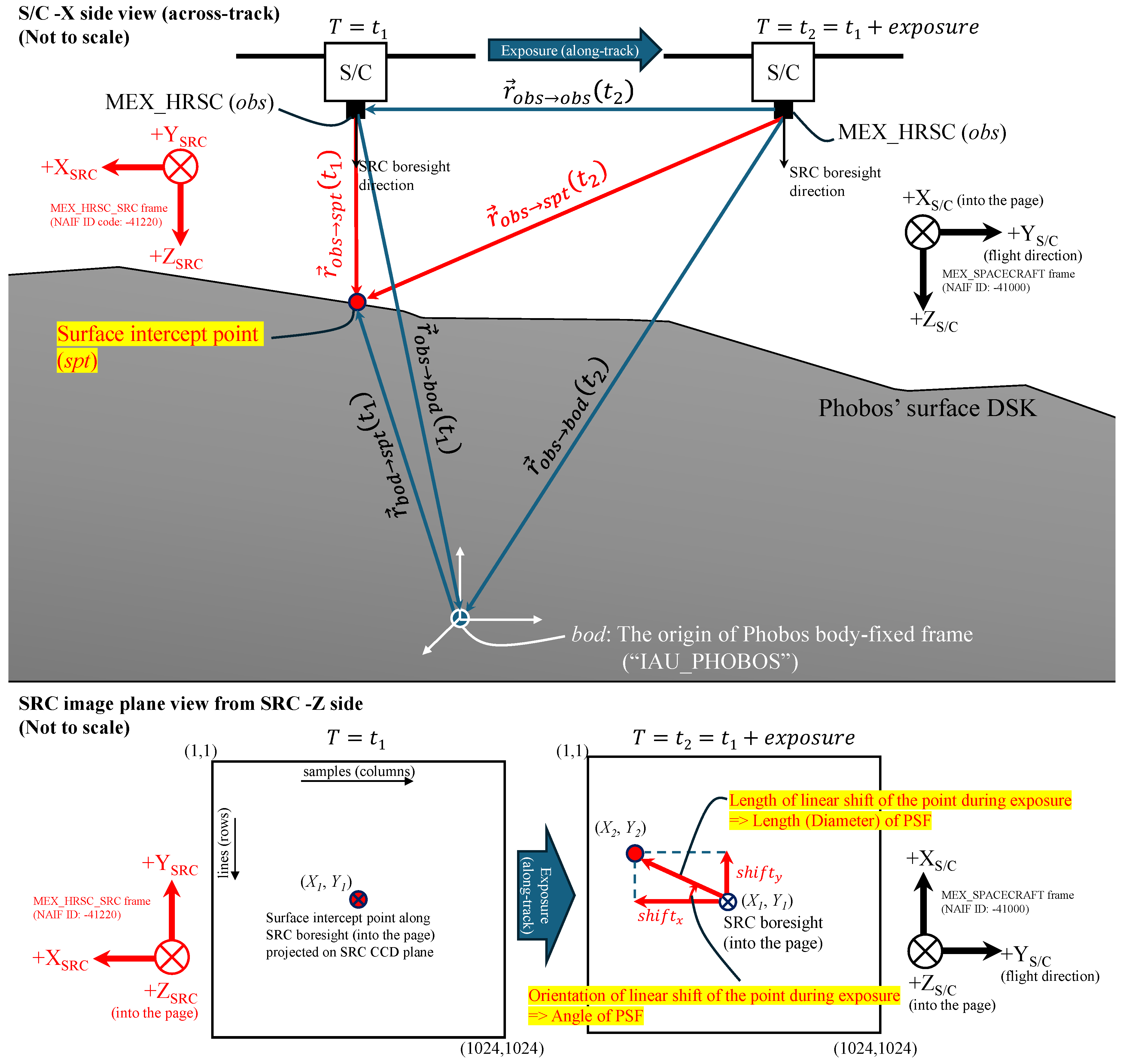
Figure 4.
Results of spatial-domain intensity of phase-shifted PSFs, calculated for each of the selected SRC images. The intensity per pixel is color-coded by intervals defined by the color bar on the right. Mostly, the highest intensity pixels lie horizontally at the center of each PSF, suggesting the along-track shift of the SRC boresight during exposure. All pixels comprising each of the PSFs are normalized so that its total energy = 1. Each window size is 150×150 pixels.
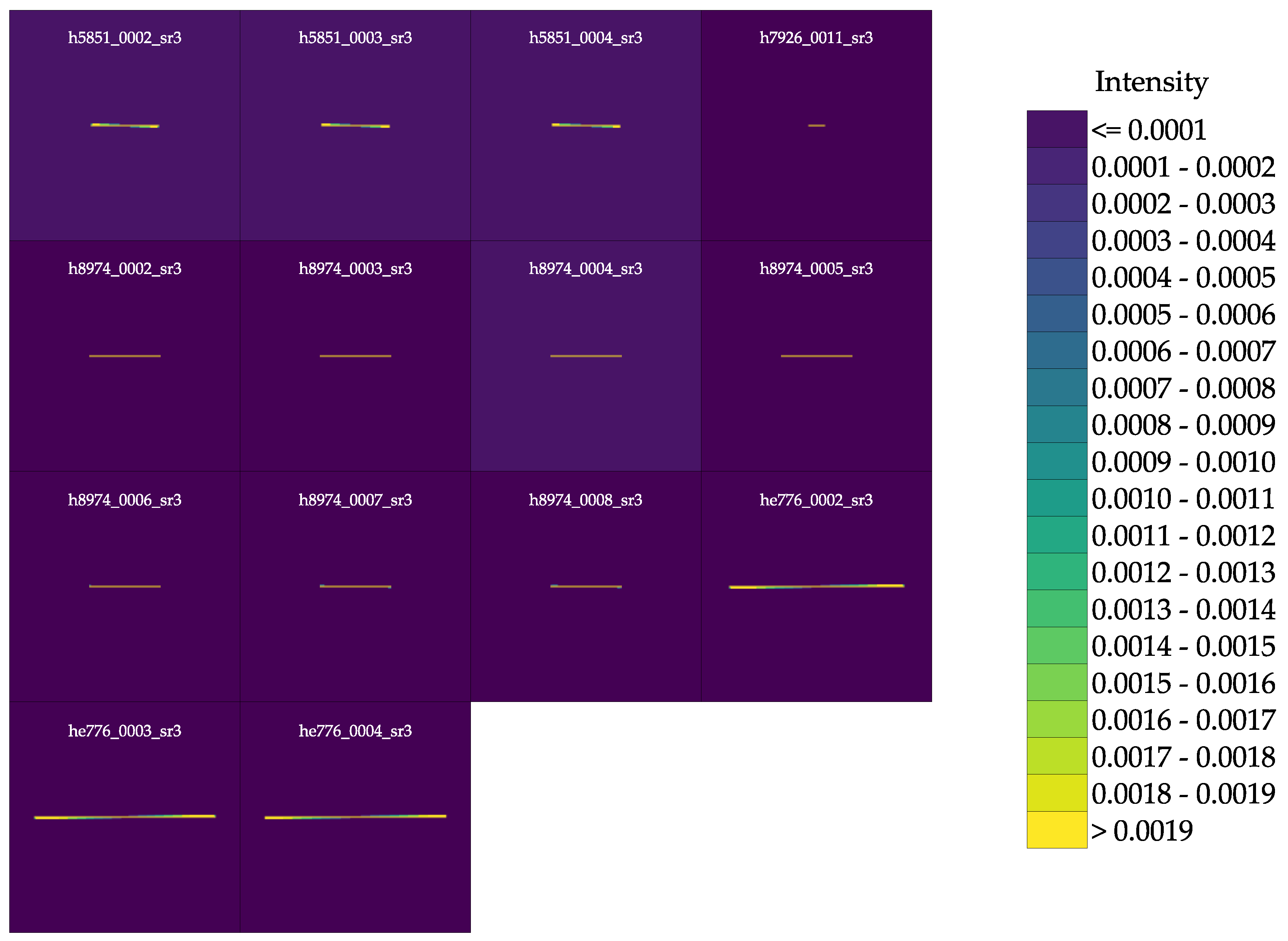
Figure 5.
The result of deconvolution about three SRC images taken in MEx orbit 5851. (a, c, e) denoised images before restoration, (b, d, f) deblurred images after restoration. Images are ordered by SRC image ID (Table 1).
Figure 5.
The result of deconvolution about three SRC images taken in MEx orbit 5851. (a, c, e) denoised images before restoration, (b, d, f) deblurred images after restoration. Images are ordered by SRC image ID (Table 1).
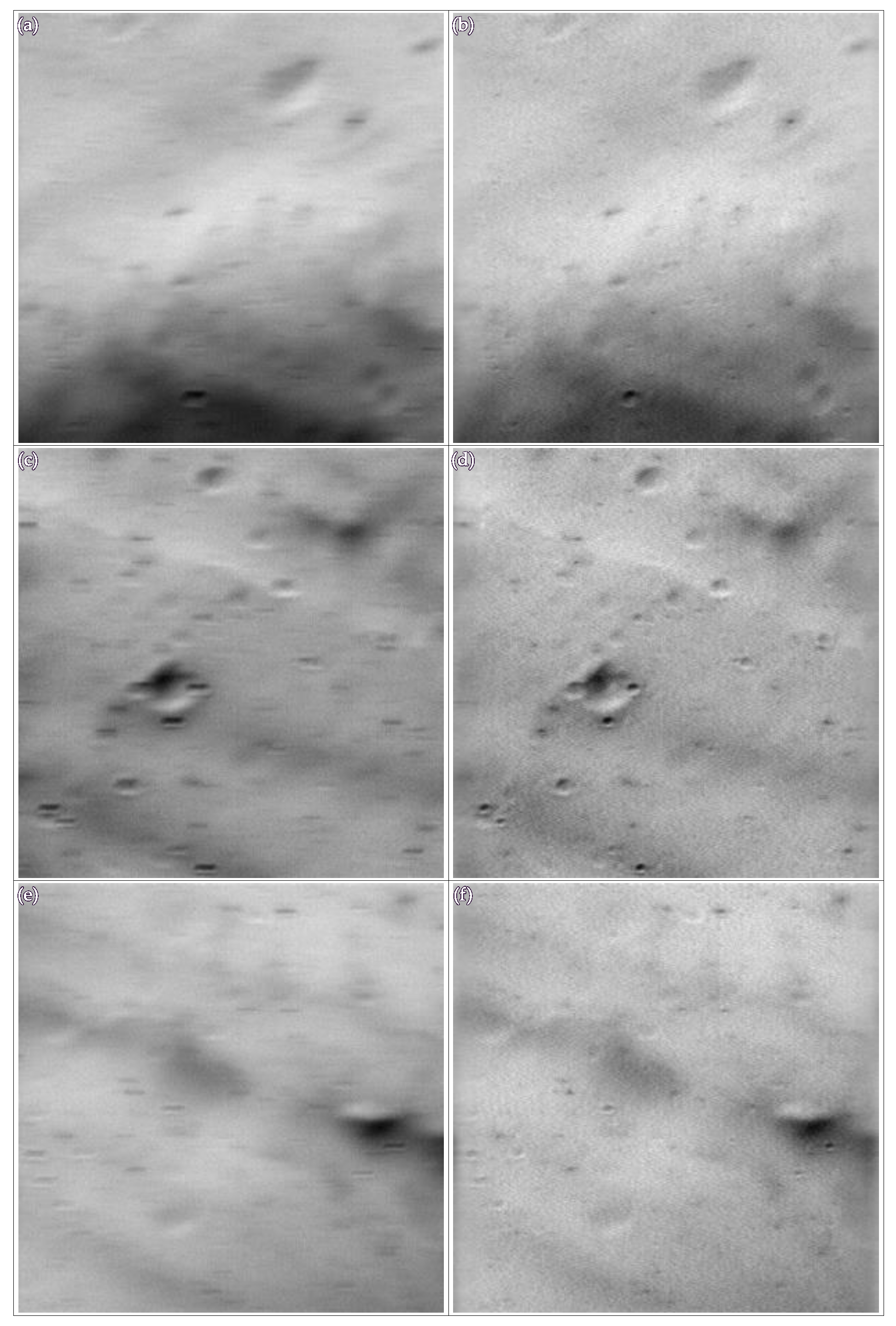
Figure 6.
The result of deconvolution about one SRC image taken in MEx orbit 7926. (a) a denoised image before restoration, (b) a deblurred image after restoration.
Figure 6.
The result of deconvolution about one SRC image taken in MEx orbit 7926. (a) a denoised image before restoration, (b) a deblurred image after restoration.
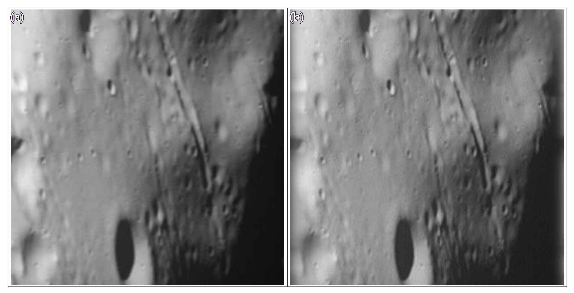
Figure 7.
The result of deconvolution about seven SRC images taken in MEx orbit 8974. (a, c, e, g, i, k, m) denoised images before restoration, (b, d, f, h, j, l, n) deblurred images after restoration. Images are ordered by SRC image ID (Table 1).
Figure 7.
The result of deconvolution about seven SRC images taken in MEx orbit 8974. (a, c, e, g, i, k, m) denoised images before restoration, (b, d, f, h, j, l, n) deblurred images after restoration. Images are ordered by SRC image ID (Table 1).
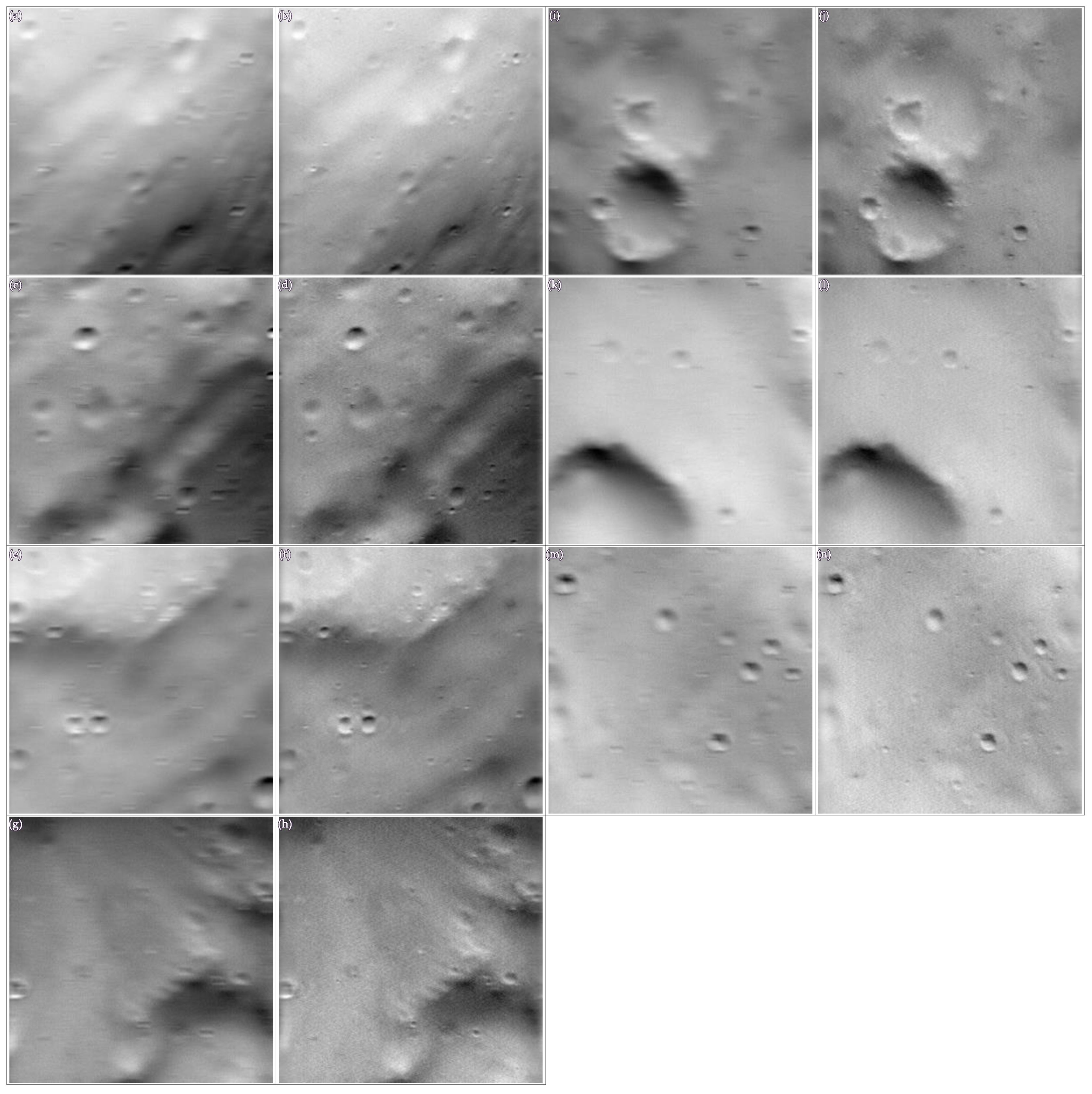
Figure 8.
The result of deconvolution about three SRC images taken in MEx orbit 14776. (a, c, e) denoised images before restoration, (b, d, f) deblurred images after restoration. Images are ordered by SRC image ID (Table 1).
Figure 8.
The result of deconvolution about three SRC images taken in MEx orbit 14776. (a, c, e) denoised images before restoration, (b, d, f) deblurred images after restoration. Images are ordered by SRC image ID (Table 1).
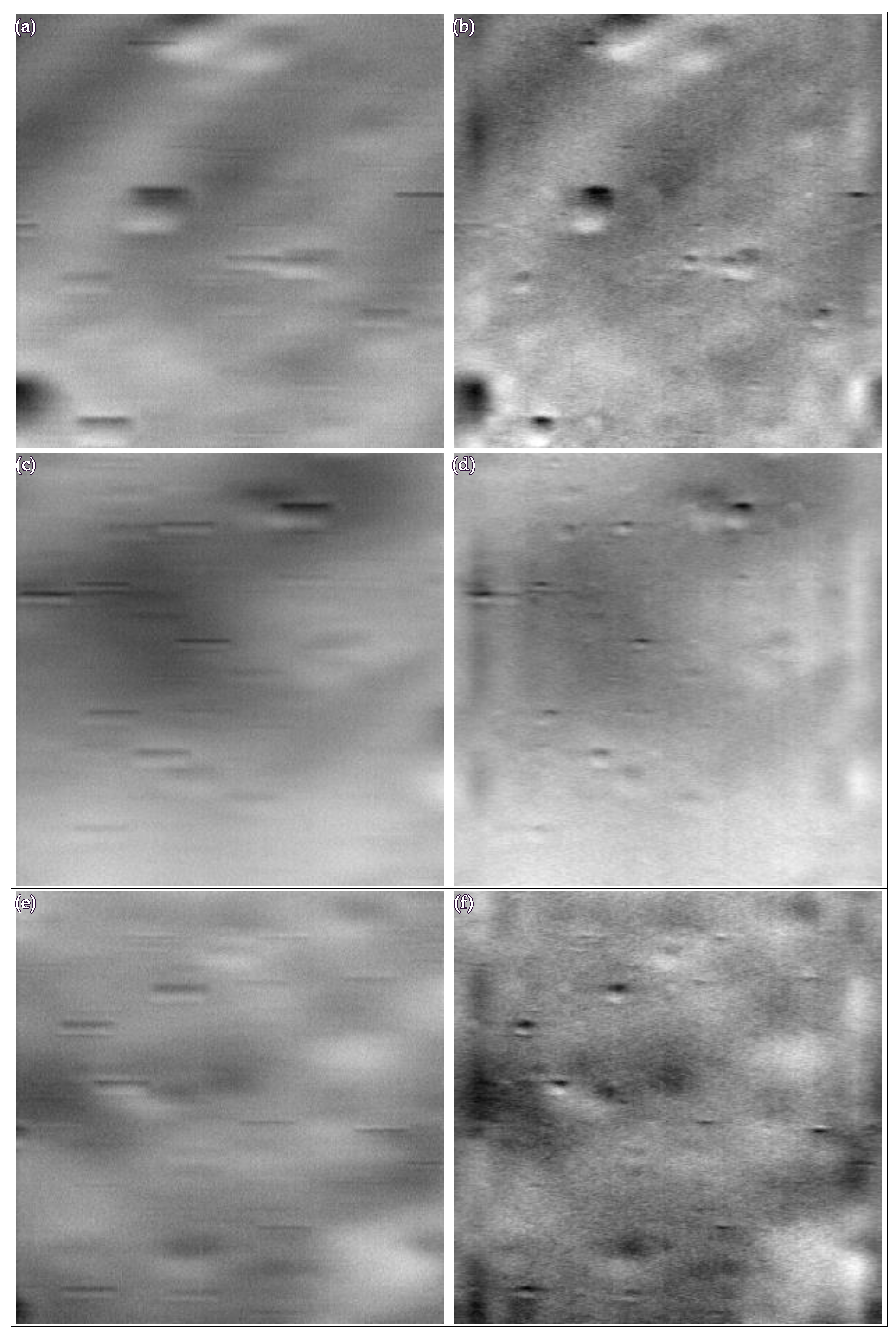

Table 1.
The list of selected MEx SRC level 3 products.
| Image ID | Longitude (°E)* | Planetocentric latitude (°N)* |
Sample resolution (meters/pixel)* |
Slant distance (km)* |
| h5851_0002_sr3 | -167.870 | 72.56 | 0.875 | 95.69 |
| h5851_0003_sr3 | 145.575 | 61.96 | 0.858 | 93.91 |
| h5851_0004_sr3 | 135.587 | 46.11 | 0.856 | 93.62 |
| h7926_0011_sr3 | 153.746 | -10.81 | 2.671 | 292.30 |
| h8974_0002_sr3 | -151.928 | -55.20 | 0.931 | 101.87 |
| h8974_0003_sr3 | -164.088 | -50.72 | 0.923 | 101.03 |
| h8974_0004_sr3 | -173.283 | -45.66 | 0.917 | 100.30 |
| h8974_0005_sr3 | 179.642 | -40.60 | 0.915 | 100.09 |
| h8974_0006_sr3 | 173.645 | -35.28 | 0.914 | 100.06 |
| h8974_0007_sr3 | 168.288 | -29.68 | 0.917 | 100.30 |
| h8974_0008_sr3 | 162.914 | -23.32 | 0.924 | 101.06 |
| he776_0002_sr3 | -29.989 | 57.82 | 0.490 | 53.66 |
| he776_0003_sr3 | 6.246 | 40.81 | 0.473 | 51.73 |
| he776_0004_sr3 | 15.872 | 31.14 | 0.468 | 51.19 |
* Values were calculated at the image center of each cube by using ISIS campt application.
Table 2.
The selected MEx SRC level 3 products with high-precision observation timings.
| Image ID |
UTC1′ ("START_TIME"with microsecond precision)* |
UTC2′ ("STOP_TIME"with microsecond precision)* |
Exposure (milliseconds) |
| h5851_0002_sr3 | 2008-07-23T04:49:59.834944 | 2008-07-23T04:49:59.849056 | 14.112 |
| h5851_0003_sr3 | 2008-07-23T04:50:00.924944 | 2008-07-23T04:50:00.939056 | 14.112 |
| h5851_0004_sr3 | 2008-07-23T04:50:02.014944 | 2008-07-23T04:50:02.029056 | 14.112 |
| h7926_0011_sr3 | 2010-03-10T05:59:39.782944 | 2010-03-10T05:59:39.797056 | 14.112 |
| h8974_0002_sr3 | 2011-01-09T14:06:28.284936 | 2011-01-09T14:06:28.301064 | 16.128 |
| h8974_0003_sr3 | 2011-01-09T14:06:28.829936 | 2011-01-09T14:06:28.846064 | 16.128 |
| h8974_0004_sr3 | 2011-01-09T14:06:29.374936 | 2011-01-09T14:06:29.391064 | 16.128 |
| h8974_0005_sr3 | 2011-01-09T14:06:29.919936 | 2011-01-09T14:06:29.936064 | 16.128 |
| h8974_0006_sr3 | 2011-01-09T14:06:30.464936 | 2011-01-09T14:06:30.481064 | 16.128 |
| h8974_0007_sr3 | 2011-01-09T14:06:31.009936 | 2011-01-09T14:06:31.026064 | 16.128 |
| h8974_0008_sr3 | 2011-01-09T14:06:31.554936 | 2011-01-09T14:06:31.571064 | 16.128 |
| he776_0002_sr3 | 2015-08-26T13:18:49.613920 | 2015-08-26T13:18:49.634080 | 20.16 |
| he776_0003_sr3 | 2015-08-26T13:18:51.248920 | 2015-08-26T13:18:51.269080 | 20.16 |
| he776_0004_sr3 | 2015-08-26T13:18:52.090920 | 2015-08-26T13:18:52.111080 | 20.16 |
* A prime symbol (′) shows a time including a microsecond precision.
Table 3.
Results of the PSF geometries as the length and orientation of spt shifts during exposure on the SRC image plane.
Table 3.
Results of the PSF geometries as the length and orientation of spt shifts during exposure on the SRC image plane.
| Image ID | shiftx (pixels) | shifty (pixels) | Length of PSF (pixels)1 | Angle of PSF (degrees)2 |
| h5851_0002_sr3 | -43.5937 | 0.2034 | 43.5942 | 179.7327 |
| h5851_0003_sr3 | -44.582 | 0.2079 | 44.5825 | 179.7328 |
| h5851_0004_sr3 | -44.8592 | 0.2016 | 44.8596 | 179.7426 |
| h7926_0011_sr3 | -11.3116 | 0.0071 | 11.3116 | 179.964 |
| h8974_0002_sr3 | 45.8297 | -0.0092 | 45.8297 | 359.9885 |
| h8974_0003_sr3 | 46.2751 | -0.0155 | 46.2751 | 359.9809 |
| h8974_0004_sr3 | 46.6702 | -0.0215 | 46.6702 | 359.9736 |
| h8974_0005_sr3 | 46.8149 | -0.0265 | 46.8149 | 359.9676 |
| h8974_0006_sr3 | 46.8688 | -0.031 | 46.8688 | 359.9621 |
| h8974_0007_sr3 | 46.7906 | -0.0348 | 46.7907 | 359.9573 |
| h8974_0008_sr3 | 46.4568 | -0.0375 | 46.4568 | 359.9538 |
| he776_0002_sr3 | 113.9898 | 0.5825 | 113.9913 | 0.2928 |
| he776_0003_sr3 | 117.8935 | 0.643 | 117.8953 | 0.3125 |
| he776_0004_sr3 | 118.8855 | 0.5837 | 118.8869 | 0.2813 |
Table 4.
Practical implications of the two deconvolution methods.
| Aspect | Wiener Deconvolution | Lucy–Richardson Deconvolution |
| Domain | Frequency | Spatial (iterative) |
| Speed | Fast: one filter application | Slower: many iterations |
| Regularization | Built-in via noise term SN/SF | Implicit via stopping rule (iterations) |
| Image Priors | Requires power spectral density estimates | Implicit Poisson model + positivity |
| Result Control | Trade-off set by noise term | Trade-off by number of iterations |
| Typical Use-case | When noise is Gaussian and PSF known | When photon-limited or low-SNR imagery |
Disclaimer/Publisher’s Note: The statements, opinions and data contained in all publications are solely those of the individual author(s) and contributor(s) and not of MDPI and/or the editor(s). MDPI and/or the editor(s) disclaim responsibility for any injury to people or property resulting from any ideas, methods, instructions or products referred to in the content. |
© 2025 by the authors. Licensee MDPI, Basel, Switzerland. This article is an open access article distributed under the terms and conditions of the Creative Commons Attribution (CC BY) license (https://creativecommons.org/licenses/by/4.0/).
Copyright: This open access article is published under a Creative Commons CC BY 4.0 license, which permit the free download, distribution, and reuse, provided that the author and preprint are cited in any reuse.


