

Submitted:
08 July 2025
Posted:
11 July 2025
You are already at the latest version
Abstract
Wireless Sensor Networks (WSNs) are a key enabling technology for modern e-Health applications. However, their deployment in clinical environments faces critical challenges due to dynamic network topologies, signal interference, and stringent energy constraints. Static resource allocation schemes often prove inadequate in these mission-critical settings, leading to communication failures that can compromise data integrity and patient safety. This paper proposes a novel hybrid framework for intelligent, dynamic resource allocation that addresses these challenges. The framework combines classical graph-coloring heuristics—Greedy and Recursive Largest First (RLF) for efficient initial channel assignment with the adaptive power of metaheuristics, specifically Simulated Annealing and Genetic Algorithms, for localized refinement. Unlike conventional approaches that require costly, network-wide reconfigurations, our method performs targeted adaptations only in interference-affected regions, thereby optimizing the trade-off between network reliability and energy efficiency. Comprehensive simulations modeled on dynamic, hospital-scale WSNs demonstrate the effectiveness of various hybrid strategies. Notably, the combination of RLF with a Genetic Algorithm achieves near-perfect interference mitigation and high data reliability while maintaining minimal adaptation latency. These results validate the proposed framework as a scalable, energy-aware solution for resilient, real-time healthcare telecommunication infrastructures.
Keywords:
Wireless Sensor Networks
; genetic algorithm
; e-health
; Recursive Largest First.
1. Introduction
Wireless Sensor Networks (WSNs) have become a fundamental technology in modern eHealth applications, enabling real-time monitoring of patients through wearable devices, bedside sensors, and ambient hospital systems. The paradigm of e-Health is rapidly transforming healthcare delivery, with recent market analyses projecting the global telehealth market to exceed $280 billion by 2025, driven by an aging global population and the rising prevalence of chronic diseases requiring continuous oversight. These networks form the backbone of a multi-tiered medical data infrastructure. At the first tier, wearable and ambient sensors such as ECG monitors, SpO2 oximeters, and glucose meters collect raw physiological data directly from the patient. This data is then transmitted to a second-tier personal server, often a smartphone or a dedicated bedside aggregator, before being relayed to third-tier cloud servers at a medical facility for analysis by healthcare professionals [1, 2]. This architecture supports continuous data collection and wireless transmission of vital health information, facilitating remote patient monitoring, chronic disease management, and timely emergency responses.
However, the clinical environments where these systems are deployed are highly dynamic. In settings like hospitals or assisted living facilities, frequent topology changes are the norm, caused by patient and staff mobility, the repositioning of medical equipment, and fluctuating environmental factors that affect radio frequency propagation [3]. These dynamics frequently disrupt network communication, causing wireless interference that corrupts data packets and leads to communication failures. The consequences of such failures in a clinical context are severe. A single lost data packet from a cardiac monitor is not merely a technical glitch; it could represent a missed arrhythmia event, delaying a life-saving intervention. Similarly, intermittent connectivity for a continuous glucose monitor could mask a dangerous hypoglycemic episode.
The "hidden cost" of this unreliability extends beyond the immediate clinical risk. Packet retransmissions, the primary mechanism to combat data loss from interference, elevate energy usage significantly a critical issue, as energy is a precious and finite resource in battery-powered sensor nodes. This directly compromises the operational lifetime of monitoring systems, necessitating more frequent battery replacements and increasing maintenance overhead [4]. Furthermore, the act of retransmitting packets increases network latency and congestion. This is particularly perilous for e-Health applications that depend on sub-200 millisecond response times for critical alerts, such as automated fall detection or cardiac distress alarms [5, 6]. The limited computational capacity of individual sensor nodes further compounds the problem, restricting their ability to rapidly adapt to network changes.
The technical heart of this challenge lies in the efficient allocation of wireless channels to minimize interference. This resource allocation problem can be formally modeled as a graph coloring problem, where sensor nodes are vertices, potential interference links between nodes are edges, and the available wireless channels are colors. The objective is to assign distinct colors (channels) to any two adjacent vertices (interfering nodes) while minimizing the total number of colors used. Determining the minimum number of colors required (the chromatic number) is a well-known NP-hard problem, making it computationally infeasible to find a perfect solution for large networks in real-time. This necessitates the use of advanced heuristic and metaheuristic methods [7, 8].
Classic graph-coloring heuristics, such as the Greedy algorithm and Recursive Largest First (RLF), offer fast and straightforward methods for an initial channel assignment. However, their static nature renders them ineffective in the face of constant network changes. They require a complete and energy-intensive re-computation for every significant topology change, making them unsuitable for real-time, dynamic WSN environments [9, 10].
To enhance adaptability, this research introduces a hybrid framework that integrates these fast graph-coloring heuristics with adaptive metaheuristics—namely Simulated Annealing (SA) and Genetic Algorithms (GA) [11, 12]. SA introduces a stochastic, "temperature-guided" exploration of the solution space, allowing it to escape local minima, while GAs evolve a population of potential channel assignments through processes of crossover and mutation, guiding the overall solution toward optimal interference reduction.
In this proposed framework, the initial channel assignment is performed using either the Greedy or RLF heuristic to establish a strong baseline configuration. Subsequently, dynamic adjustments triggered by topology changes detected by a centralized base station employ SA or GA for localized recoloring. This targeted adaptation avoids the need for a full, network-wide recalculation of the channel map. By combining these strategies, the system aims to strike a crucial balance between initial efficiency, adaptive robustness, and energy conservation, all of which are essential for the demanding conditions of densely populated and highly mobile e-Health environments [13].
The framework's performance is evaluated through a comprehensive, simulation-driven approach that models a 50×50-meter hospital ward with 100 sensor nodes, 20% of which are mobile. Key performance indicators including energy consumption, interference rate, packet loss, and adaptation latency are meticulously tracked over multiple mobility events to assess the efficacy of each algorithmic combination. This methodology ensures the practical relevance of the findings by reflecting the conditions of real-world e-Health deployments.
2. Literature Review
This section provides a comprehensive review of the existing literature pertinent to resource allocation in dynamic Wireless Sensor Networks (WSNs), with a specific focus on applications in e-Health. It begins by examining the fundamental challenges posed by dynamic network environments and establishes graph coloring as a classical approach to interference management. It then delves into the application of various metaheuristic algorithms for WSN optimization, offers a comparative analysis, and justifies the selection of Simulated Annealing (SA) and Genetic Algorithms (GA) for this research. Additionally, it discusses the importance of Quality of Service (QoS) and scalability in healthcare contexts, identifies critical gaps in the current body of research, and situates the contribution of this research within the broader academic landscape.
The successful deployment of WSNs in healthcare settings is contingent upon their ability to operate reliably in environments characterized by constant change. Authors at [14] highlight that node mobility, whether from ambulatory patients or mobile medical equipment, is a primary source of network instability. Their work surveys various bio-inspired algorithms for managing dynamic resource allocation, concluding that adaptability is the most critical feature for maintaining network performance. Similarly, authors at [3] provide a thorough survey on mobility management protocols in Wireless Body Area Networks (WBANs), a subset of WSNs. They categorize mobility into predictable (e.g., a patient walking down a hallway) and unpredictable (e.g., erratic movements during a medical emergency) patterns, emphasizing that MAC protocols must be robust enough to handle both without significant degradation in data delivery. A key takeaway from their analysis is that frequent topology changes lead to a cascade of problems, including route invalidation, increased control overhead, and a surge in co-channel interference.
The problem of assigning wireless channels to nodes to minimize interference is canonically modeled as a graph coloring problem. The foundational work by [8] provides a comprehensive review of this technique's application in both wired and wireless networks. They establish the formal equivalence between channel assignment and graph coloring, where nodes are vertices, an interference link is an edge, and channels are colors. Their review confirms that graph coloring provides an elegant and mathematically rigorous framework for abstracting this complex engineering problem. While exact solutions are NP-hard, they note the widespread use and effectiveness of heuristics.
Building on this, authors at [10] have applied graph coloring to real-world WiFi scenarios, demonstrating tangible performance improvements. Their approach combined graph contraction techniques with an SA-based coloring algorithm, which resulted in a measurable increase in network throughput and a reduction in interference. However, their work primarily focused on semi-static WiFi networks and did not fully address the continuous, small-scale mobility found in dense WSNs. Furthermore, authors at [9] explore energy-aware scheduling in the Internet of Medical Things (IoMT) using coloring heuristics. Their findings indicate that while heuristics like Greedy and RLF are computationally efficient for initial setup, their performance degrades sharply in dynamic scenarios, necessitating frequent, energy-intensive network-wide re-colorings, thus motivating the need for more adaptive solutions.
Given the limitations of static heuristics, researchers have increasingly turned to metaheuristics high-level problem-independent algorithmic frameworks that provide a set of guidelines or strategies to develop heuristic optimization algorithms. Simulated Annealing (SA) is a probabilistic technique for approximating the global optimum of a given function. Its strength lies in its ability to escape local optima by accepting worse solutions with a probability that decreases over time, governed by a "temperature" parameter. In the context of WSNs, authors at [15] proposed an efficient hybrid SA-DSATUR method. Their model used SA to refine the channel assignments produced by the DSATUR heuristic, achieving a better balance between the number of channels used and computational overhead. Their results showed a significant reduction in conflicts compared to DSATUR alone. The primary limitation noted was the sensitivity of SA to its cooling schedule, a schedule that is too fast may cause the algorithm to converge prematurely to a suboptimal solution. Furthermore, Genetic Algorithm (Gas) is a class of evolutionary algorithms that use principles of natural selection to find optimal solutions. They operate on a population of potential solutions, applying operators like selection, crossover, and mutation. Authors in [16] provide a comprehensive survey on the use of GAs in wireless networks, highlighting their flexibility in handling dynamic and multi-objective optimization problems, such as balancing energy consumption and network coverage. More recently, authors at [17] developed a GA-based self-healing mechanism for WSNs in mission-critical healthcare. Their GA dynamically re-routes traffic and re-establishes connectivity in response to node failures, demonstrating the algorithm's robustness. A key challenge with GAs is parameter tuning (e.g., population size, mutation rate), which can significantly impact performance and convergence speed.
While this research work focuses on SA and GA, other nature-inspired algorithms are prominent in WSN literature. Particle Swarm Optimization (PSO) is a population-based stochastic optimization technique inspired by the social behavior of bird flocking or fish schooling. Each "particle" in the swarm adjusts its trajectory based on its own best-known position and the best-known position of the entire swarm. PSO is known for its fast convergence but can sometimes converge prematurely to local optima in highly complex, multi-modal search spaces. Additionally, Ant Colony Optimization (ACO) is inspired by the foraging behavior of ants, who deposit pheromones on the ground to mark favorable paths for the colony. It is particularly well-suited for finding optimal paths in graphs and has been extensively applied to routing problems in WSNs. However, for a channel assignment problem, which is less about pathfinding and more about constraint satisfaction, the mapping to an ACO framework is less direct than with GA or SA. For the dynamic channel assignment problem, SA and GA were chosen for specific reasons. Simulated Annealing was selected for its simplicity and its proven ability to perform effective local searches. In our hybrid model, where a good solution from a heuristic is already in place, SA is ideally suited to explore the immediate neighborhood of that solution for incremental improvements. Genetic Algorithms were chosen for their strength in parallel exploration of the solution space. When a localized adaptation is needed, the GA can maintain a diverse population of potential new channel configurations for the affected nodes, increasing the likelihood of finding a robust solution that does not just solve the immediate conflict but is also resilient to future changes. In contrast, PSO's rapid convergence was seen as a potential drawback, while ACO was deemed a less natural fit for a constraint-based assignment problem compared to a routing problem.
The literature strongly suggests that hybrid models often outperform standalone algorithms. Authors at [18] demonstrated this by using SA as part of a hybrid model for cluster head selection in WSNs. By using SA to refine the clustering decisions, they significantly extended network lifetime compared to traditional hierarchical protocols. Authors in [19] explicitly combined SA and GA for dynamic channel allocation, showing that the hybrid approach could adapt to heterogeneous network conditions more effectively than either algorithm alone. The core insight from this body of work is that hybridization allows a system to leverage the complementary strengths of different algorithms for instance, using a fast heuristic for an initial solution and a more computationally intensive metaheuristic for refinement. This is the central premise of the framework proposed in this research work.
Another important aspect is related to quality of Services (QoS) in e-Health where WSNs refers to the network's ability to provide a guaranteed level of performance, which is critical when dealing with medical data [20-25]. Key QoS metrics include:
- Reliability: The guarantee that data packets are delivered successfully. High interference directly degrades reliability.
- Timeliness (Latency): The time taken for a packet to travel from sensor to sink. As noted by [26], some critical medical alerts require latency below 200ms.
- Data Accuracy: Ensuring the delivered data is not corrupted.
Any resource allocation strategy must be evaluated against these QoS requirements. A low-energy solution is useless if it cannot deliver data reliably and in a timely manner.
Scalability is another critical concern. As hospitals and healthcare facilities deploy more sensor devices, the network size can grow to hundreds or even thousands of nodes. A resource allocation strategy that works for 20 nodes may fail completely at a scale of 200. This is where the concept of localized adaptation becomes essential. Strategies that require a global, network-wide recalculation of channels for every minor change will not scale. They create a massive communication overhead and drain network energy. The research gap in developing scalable, localized adaptation mechanisms is a key area this research work aims to address.
Based on this comprehensive review, several critical research gaps have been identified:
- Lack of Focus on Interference-Centric Hybrid Models: While hybrid models exist, they often focus on energy conservation in the context of routing or clustering. Few studies have developed hybrid models specifically targeting the dynamic channel assignment problem using a combination of classical graph-coloring heuristics and adaptive metaheuristics.
- Predominance of Full-Network Adaptation: Most existing models, when faced with a topology change, resort to a full reassignment of resources across the entire network. The concept of lightweight, localized recoloring where only the nodes directly affected by a change are adapted is significantly underexplored.
- Limited Comparative Analysis: There is a scarcity of comprehensive, side-by-side comparisons of different hybrid combinations (e.g., Greedy+SA vs. RLF+GA) evaluated under realistic, dynamic mobility patterns and assessed across a balanced set of metrics including conflict rate, energy, latency, and packet loss.
This literature review confirms that managing interference in dynamic e-Health WSNs is a complex, multi-faceted challenge. Graph coloring provides a solid theoretical foundation, while metaheuristics like SA and GA offer powerful tools for optimization. However, existing research has not adequately addressed the need for a scalable, energy-efficient, and low-latency solution that can adapt to the continuous mobility inherent in clinical environments. This research work positions itself to fill these identified gaps by proposing and evaluating a novel hybrid framework. By combining the speed of RLF and Greedy coloring for initial setup with the intelligent, localized adaptation of SA and GA, this research aims to provide a practical and robust solution that explicitly balances the competing demands of performance, energy, and latency, thereby advancing the development of reliable communication infrastructures for next-generation e-Health systems.
3. Methodology
This section details the systematic methodology employed to design, implement, and evaluate the proposed hybrid framework for dynamic resource allocation. The approach is rooted in a robust, custom-built simulation environment that allows for the controlled comparison of various algorithmic strategies under realistic e-Health operational conditions. The methodology is presented in several parts: first, an overview of the hybrid simulation framework and its architecture; second, a detailed specification and justification of the simulation parameters and models; third, an in-depth explanation of the graph-coloring and metaheuristic algorithms implemented; fourth, a discussion of the software design principles used; and finally, a definition of the performance metrics used for evaluation.
3.1. Hybrid Simulation Framework Architecture
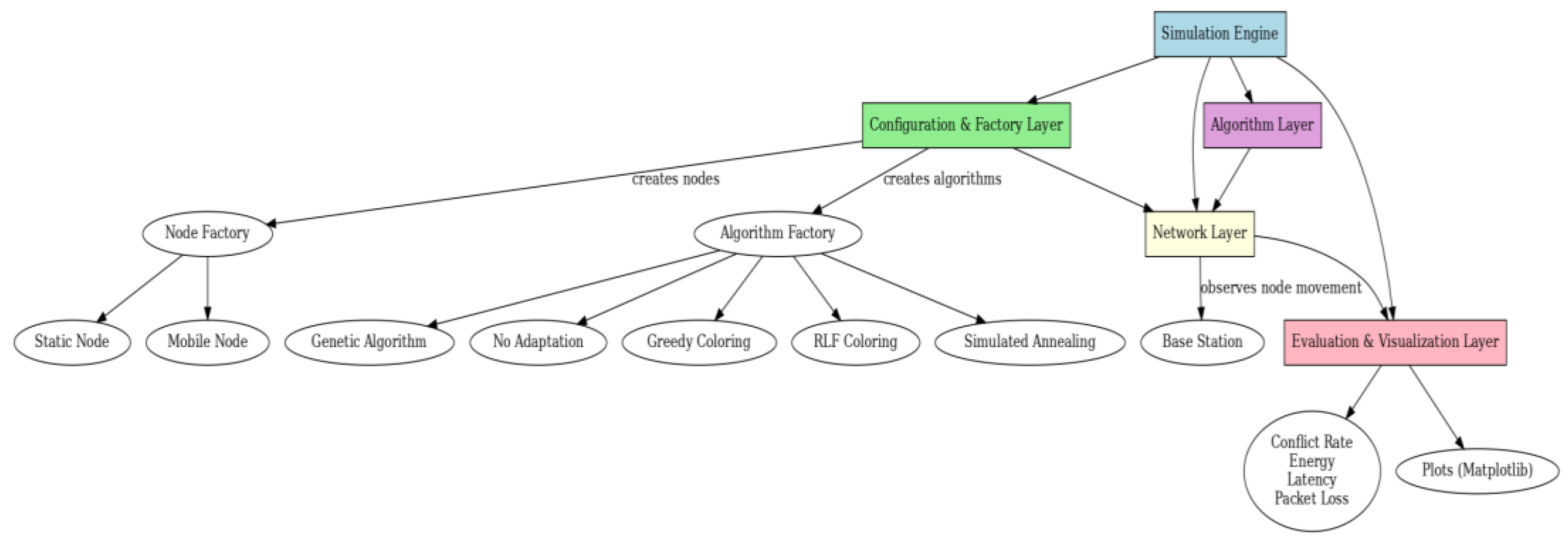
A modular, object-oriented simulation framework was developed in Python to serve as the testbed for this research. The architecture is designed for extensibility and clarity, comprising several core components whose interactions are governed by established software design patterns.
- Sensor Nodes (Node classes): Represent the fundamental network entities. An abstract base class Node defines common attributes like node_id, position, and energy. This is extended by two concrete classes: StaticNode and MobileNode, reflecting the different device types in a hospital setting. This class hierarchy allows for polymorphism in the simulation logic.
- Network (Network class): Acts as a container for all nodes and serves as the environment model. It manages the spatial relationships between nodes, computes interference graphs, and maintains a history of performance metrics for later analysis.
- Base Station (BaseStation class): Functions as the centralized controller and intelligence of the network. It implements the Observer design pattern, "listening" for mobility events from MobileNode instances. Upon receiving a notification of a topology change, it assesses the new interference landscape and triggers the appropriate adaptation algorithm. This decouples the nodes' movement from the adaptation logic, promoting modularity.
- Algorithm Modules (Algorithm classes): The core logic for channel assignment is encapsulated using the Strategy design pattern. Abstract base classes, ColoringAlgorithm and AdaptationAlgorithm, define a common interface for initial coloring and dynamic adaptation, respectively. Concrete strategy classes (e.g., GreedyColoring, RLFColoring, SimulatedAnnealingAdaptation, GeneticAlgorithmAdaptation) implement this interface. This design allows the simulation to be easily configured with any combination of initial coloring and adaptation algorithms without changing the core simulation logic.
- Metric Recorder: Integrated within the Network class, this component logs key performance indicators (KPIs) at each discrete simulation step. Time-series data for each metric is stored, facilitating the generation of comparative performance graphs.
This architecture ensures that the simulation is both a faithful representation of a WSN and a flexible research tool for algorithmic evaluation, see Fig. 1.
Figure 1.
Architecture diagram of the simulation.
3.2. Simulation Environment and Parameters
To ensure the reproducibility and relevance of the experimental results, the simulation environment was configured with a consistent set of parameters, detailed in Table 1.
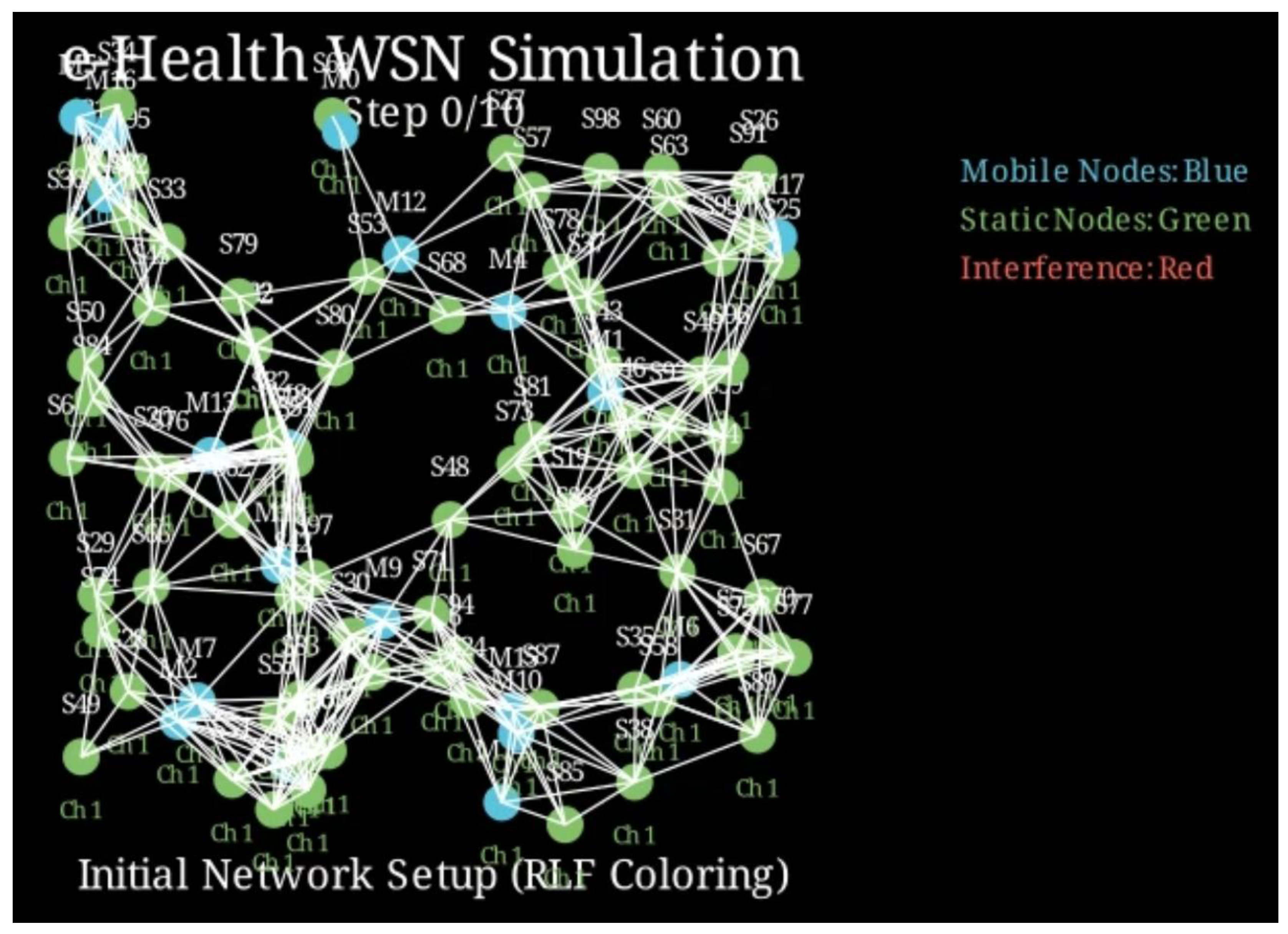
Additionally, Fig. 2 depict the real visual view of architecture that we have implemented.
Figure 2.
Real visual view of architecture implementation.
3.3. Network and Energy Models
3.3.1. Interference Model
Interference is modeled based on the graph representation of the network. An interference graph G = (V, E) is constructed where V is the set of all sensor nodes. An edge (u, v) exists in E if the Euclidean distance between nodes u and v is less than or equal to the INTERFERENCE_RANGE. A conflict occurs between two nodes u and v if an edge (u, v) exists in E and both nodes are assigned the same channel. The total number of conflicts in the network is the number of such interfering pairs.
3.3.2. Energy Consumption Model
The energy model is designed to account for the primary sources of power consumption in a WSN: communication and computation. The costs are defined as relative measures to compare the algorithmic overhead.
- Communication Energy (ENERGY_MESSAGE): A small, fixed cost is deducted every time a node sends a message (e.g., when a mobile node notifies the base station of its new position). This represents the energy for radio transmission.
- Computation Energy (Algorithmic Costs): The energy costs for running the algorithms (ENERGY_GREEDY, ENERGY_RLF, ENERGY_SA, ENERGY_GA) are estimates representing their relative computational complexity. For instance, ENERGY_RLF (10.0 mJ) is set higher than ENERGY_GREEDY (5.0 mJ) to reflect RLF's higher computational demand. Similarly, ENERGY_GA (1.5 mJ) is higher than ENERGY_SA (1.0 mJ) because it involves managing a population of solutions. These costs are crucial for evaluating the trade-off between achieving a better channel assignment and conserving node energy. For the initial coloring algorithms, this cost is distributed evenly among all nodes in the network. For adaptation, the cost is borne solely by the mobile node performing the computation.
3.4. Initial Channel Assignment Heuristics
Two classical graph-coloring heuristics were implemented to provide the initial, conflict-free channel map.
3.4.1. Greedy Algorithm
The Greedy algorithm is a simple and fast heuristic that iterates through the nodes in a sequential order and assigns each node the first available channel that is not being used by any of its already-colored neighbors.
- Logic: Its primary advantage is its low computational complexity, but its performance is highly dependent on the initial ordering of the nodes, often leading to suboptimal channel usage.
- Computational Complexity: O(V*Δ), where V is the number of vertices and Δ is the maximum degree of the graph.
Algorithm 1 is focused on Greedy Coloring where the input and output data are as follows:
- Input: Network G = (V, E), Number of Channels K
- Output: A channel assignment for all nodes in V
- 1: for each node u in V do
- 2: neighbor_channels ← {channel of v | (u,v) in E and v is colored}
- 3: for channel c from 0 to K-1 do
- 4: if c is not in neighbor_channels then
- 5: u.channel ← c
- 6: break
- 7: end if
- 8: end for
- 9: end for
3.4.2. Recursive Largest First (RLF) Algorithm
RLF is a more sophisticated heuristic that attempts to produce a more optimal coloring by prioritizing nodes that are more "difficult" to color.
- Logic: It works by iteratively building sets of nodes that can share the same color. In each iteration, it selects an uncolored node with the highest degree (most neighbors). This node becomes the first member of a new color class. It then greedily adds other uncolored nodes to this class, ensuring that no two nodes in the class are neighbors. This process is repeated until all nodes are colored.
- Computational Complexity: Typically, O(V²), as it may require multiple passes over the node set.
Algorithm 2 is focused on Recursive Largest First (RLF) Coloring where the input and output data are as follows:
- Input: Network G = (V, E), Number of Channels K
- Output: A channel assignment for all nodes in V
- 1: Uncolored_Nodes ← V
- 2: c ← 0
- 3: while Uncolored_Nodes is not empty do
- 4: Color_Class ← {}
- 5: // Select node with max degree in the remaining graph
- 6: u ← node in Uncolored_Nodes with max degree
- 7: Add u to Color_Class
- 8: Remove u from Uncolored_Nodes
- 9:
- 10: // Add more nodes to the current color class
- 11: for each node v in Uncolored_Nodes do
- 12: // Check if v is not a neighbor to any node already in Color_Class
- 13: if (v,w) is not in E for all w in Color_Class then
- 14: Add v to Color_Class
- 15: Remove v from Uncolored_Nodes
- 16: end if
- 17: end for
- 18:
- 19: // Assign the current channel to all nodes in the class
- 20: for each node x in Color_Class do
- 21: x.channel ← c
- 22: end for
- 23: c ← c + 1
- 24: end while
3.5. Metaheuristic Adaptation Algorithms
Two metaheuristics were implemented for the dynamic adaptation phase, triggered when a mobile node creates a new conflict.
3.5.1. Simulated Annealing (SA) Adaptation
SA is used for its effectiveness in local search problems.
- Logic: Starting with the mobile node's current (conflicting) channel, SA iteratively explores new random channels. A new channel is always accepted if it reduces the number of conflicts. If it does not, it may still be accepted based on a probability P = exp(-ΔC / T), where ΔC is the change in the number of conflicts and T is the current "temperature." The temperature starts high and is gradually lowered according to a "cooling schedule." This allows the algorithm to escape local optima early on and converge to a good solution as the temperature drops.
-
Fitness Function: The cost function is simply the number of conflicts a given channel assignment for the mobile node would create. The goal is to minimize this cost.Algorithm 3 is focused on Simulated Annealing (SA) Adaptation where the input and output data are as follows:
- Input: Network G, mobile_node m, Initial Temperature T_max, Cooling Rate α
- Output: An updated channel for m
- 1: current_channel ← m.channel
- 2: best_channel ← current_channel
- 3: T ← T_max
- 4: for i from 1 to MAX_ITERATIONS do
- 5: new_channel ← random channel from 0 to K-1
- 6: current_cost ← count_conflicts(m, current_channel)
- 7: new_cost ← count_conflicts(m, new_channel)
- 8:
- 9: if new_cost < current_cost then
- 10: current_channel ← new_channel
- 11: else if random(0,1) < exp((current_cost - new_cost) / T) then
- 12: current_channel ← new_channel
- 13: end if
- 14:
- 15: if count_conflicts(m, current_channel) < count_conflicts(m, best_channel) then
- 16: best_channel ← current_channel
- 17: end if
- 18:
- 19: T ← T * α // Cool down
- 20: end for
- 21: m.channel ← best_channel
3.5.2. Genetic Algorithm (GA) Adaptation
GA is used for its ability to explore a diverse set of solutions in parallel.
- Logic:
- 1)
- Representation: A "chromosome" is an integer representing a channel number.
- 2)
- Initialization: A population of POP_SIZE chromosomes (random channels) is created.
- 3)
- Fitness Function: The fitness of a chromosome (channel) is calculated as 1 / (1 + num_conflicts). A conflict-free channel will have a fitness of 1.0.
- 4)
- Evolution: For a set number of GENERATIONS, a new population is created through:
- Selection: Parents are selected from the current population using roulette wheel selection, where individuals with higher fitness have a higher probability of being chosen.
- Crossover: Two parents produce two offspring. A simple swap crossover is used.
- Mutation: Each offspring has a small probability (MUTATION_RATE) of being changed to a new random channel.
- The best chromosome from the final population is chosen as the new channel for the mobile node.
Algorithm 4 is focused on Genetic Algorithm (GA) Adaptation where the input and output data are as follows:
- Input: Network G, mobile_node m, Population Size N, Generations G_max
- Output: An updated channel for m
- 1: Population ← Initialize N random channels
- 2: for i from 1 to G_max do
- 3: // Calculate fitness for each individual in the population
- 4: Fitness_Scores ← [1 / (1 + count_conflicts(m, channel)) for channel in Population]
- 5:
- 6: New_Population ← {}
- 7: for j from 1 to N/2 do
- 8: // Select two parents based on fitness
- 9: parent1 ← RouletteWheelSelect(Population, Fitness_Scores)
- 10: parent2 ← RouletteWheelSelect(Population, Fitness_Scores)
- 11:
- 12: // Crossover and Mutation
- 13: child1, child2 ← Crossover(parent1, parent2)
- 14: Mutate(child1)
- 15: Mutate(child2)
- 16: Add child1, child2 to New_Population
- 17: end for
- 18: Population ← New_Population
- 19: end for
- 20:
- 21: // Return the best individual from the final population
- 22: Final_Fitness_Scores ← [1 / (1 + count_conflicts(m, channel)) for channel in Population]
- 23: best_channel ← channel in Population with max fitness
- 24: m.channel ← best_channel
3.6. Performance Metrics Selection
To provide a holistic and balanced evaluation of the different hybrid strategies, a set of four key performance indicators was selected, each targeting a different aspect of network quality.
- Average Conflict Rate: This is the primary metric for measuring the effectiveness of interference mitigation. It is calculated as the total number of conflicting links divided by the total number of nodes. A lower value indicates a more stable and efficient channel assignment.
- Total Energy Remaining: This metric tracks the aggregate energy of all nodes in the network over time. It directly measures the energy cost of the different algorithmic strategies, highlighting the trade-off between computational effort and energy conservation.
- Adaptation Latency: This measures the simulated time taken for the SA or GA algorithm to execute upon detecting a conflict. It is a critical metric for assessing the suitability of the framework for real-time applications where rapid adaptation is essential.
- Packet Loss Rate: This metric provides a tangible measure of the impact of interference on data delivery. In the simulation, it is modeled as being proportional to the number of conflicts, representing the increased probability of packet collisions and corruption in a congested channel.
4. Simulation Results
This section presents the empirical results obtained from the simulation framework detailed in the previous section. The performance of six distinct algorithmic combinations formed by pairing two initial coloring heuristics (Greedy, RLF) with three adaptation strategies (None, SA, GA) was evaluated over ten discrete mobility steps. The analysis focuses on four key performance indicators: conflict rate, packet loss rate, total energy remaining, and adaptation latency. The findings are presented through a series of comparative figures, followed by a detailed interpretation of the quantitative outcomes.
The simulation results unequivocally demonstrate that the hybrid strategies combining a robust initial coloring with a metaheuristic adaptation mechanism significantly outperform static approaches in a dynamic WSN environment. The SA_RLF and GA_RLF combinations emerged as the most effective, consistently maintaining superior network stability and performance across all metrics.
The baseline strategies (None_Greedy and None_RLF), which performed no adaptation after the initial channel assignment, proved incapable of handling node mobility. Their performance degraded progressively as conflicts accumulated, underscoring the necessity of a dynamic adaptation layer. In contrast, the introduction of SA and GA as adaptation mechanisms led to dramatic improvements in interference mitigation and, consequently, overall network reliability. The choice of the initial coloring heuristic also had a discernible impact, with the more sophisticated RLF algorithm providing a consistently better foundation for the subsequent metaheuristic adaptations than the simpler Greedy algorithm.
The graphs of the Fig. 3 until 6 provide a granular analysis of each performance metric, interpreting the trends and quantitative data illustrated.
Figure 3.
Conflict Rate Over Time.
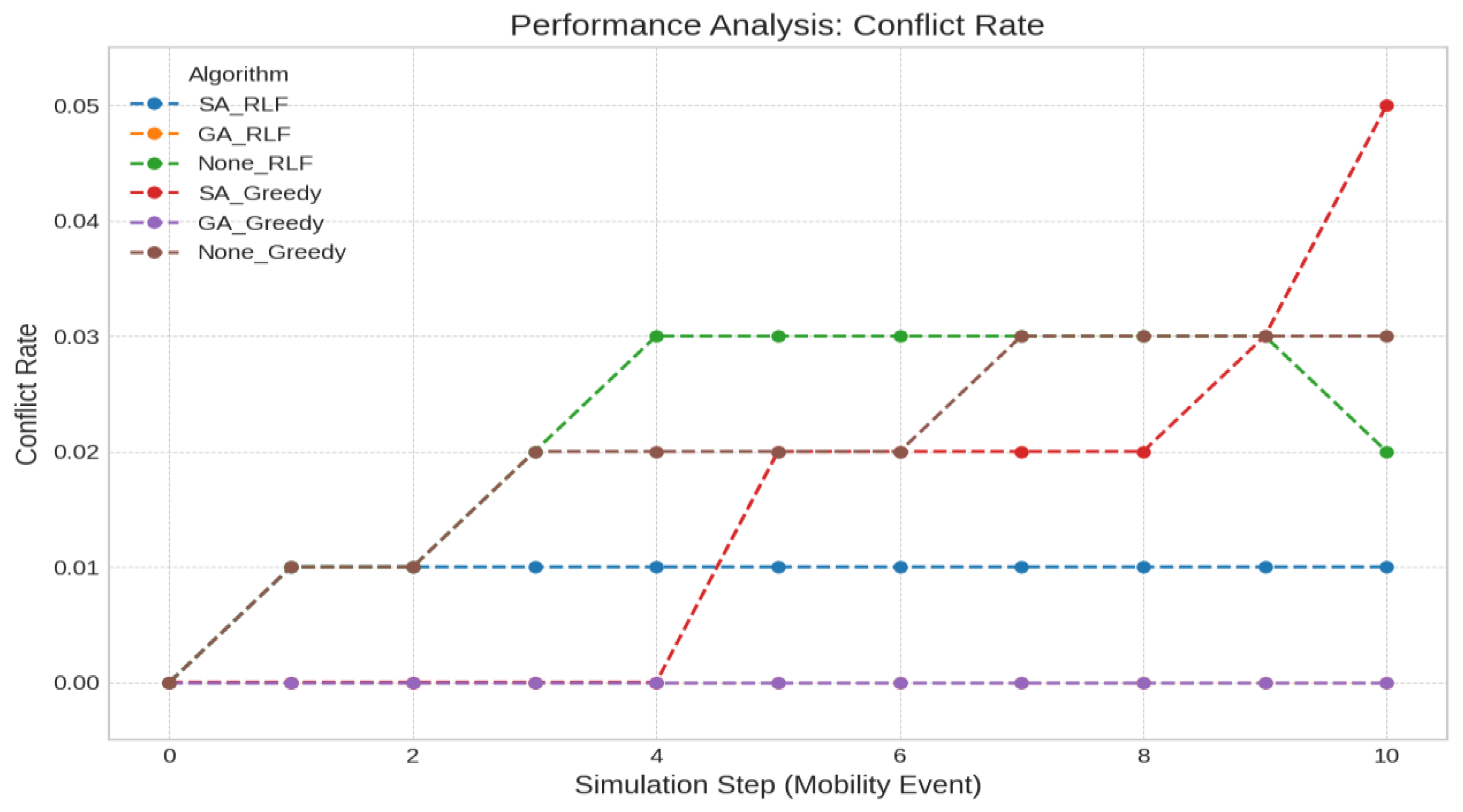
Fig. 3 clearly bifurcates the strategies into two performance tiers: adaptive and non-adaptive. The non-adaptive strategies (None_RLF and None_Greedy) exhibit a characteristic stepwise increase in conflicts. Each step corresponds to a mobility event where a new, unresolved interference link is created. By the final simulation step, the None_Greedy strategy reaches a conflict rate of approximately 0.03, while None_RLF ends slightly lower at 0.02, reflecting its more efficient initial channel map.
The adaptive strategies demonstrate remarkable effectiveness. The SA_RLF and GA_RLF combinations maintain near-zero or very low conflict rates throughout the simulation. For instance, SA_RLF sustains a conflict rate of just 0.01 after step 4, representing a 67% reduction in conflicts compared to the None_Greedy baseline at the end of the simulation. The GA_RLF strategy performs even better, maintaining a conflict rate of 0.00 for the entire duration, effectively eliminating all mobility-induced interference.
The results validate that metaheuristic adaptation is essential for interference management. The superiority of the RLF-based hybrids (SA_RLF, GA_RLF) over their Greedy-based counterparts (SA_Greedy, GA_Greedy) highlights the synergistic benefit of combining a strong initial heuristic with a powerful adaptive algorithm.
The trends in the Fig. 4 perfectly mirror those of the conflict rate, as packet loss is modeled as a direct consequence of interference. The non-adaptive strategies show a deteriorating packet loss rate that would be unacceptable for any e-Health application transmitting critical data.
The adaptive strategies, by suppressing conflicts, ensure high data fidelity. The GA_RLF strategy's ability to maintain a zero-conflict rate translates directly to a zero-packet loss rate, representing a perfect reliability score within the simulation's model. The SA_RLF strategy also maintains a very low packet loss rate of approximately 0.005. In a clinical context, this difference is significant; it is the difference between a highly reliable network and a virtually flawless one.
For QoS-sensitive applications like e-Health monitoring, proactive, metaheuristic-driven channel adaptation is not merely an optimization but a fundamental requirement for ensuring data integrity and reliability.
Figure 4.
Packet Loss Rate Over Time.

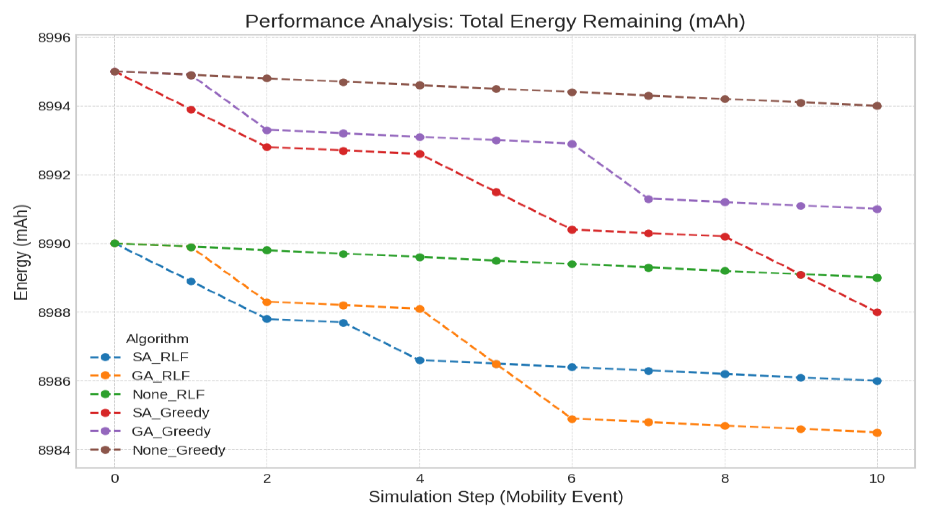
Figure 5 reveals the inherent trade-off between performance and energy consumption. The non-adaptive strategies (None_RLF, None_Greedy) are the most frugal, consuming energy only for the initial coloring and minimal message passing. In contrast, the adaptive strategies exhibit a steeper decline in energy due to the computational cost of invoking SA or GA.
The initial energy drop at step 0 is more significant for the RLF-based strategies (consuming 10.0 mJ) than the Greedy-based ones (5.0 mJ). Subsequently, each adaptation by SA (1.0 mJ) or GA (1.5 mJ) causes a further decrease in energy. While the adaptive strategies consume more direct computational energy, it is crucial to recognize that this is only part of the story. In a real-world scenario, the high conflict rates of the non-adaptive strategies would lead to constant packet retransmissions, resulting in far greater energy expenditure over time.
The GA_RLF strategy, despite having the highest computational cost per adaptation, proves to be the most effective overall. It "spends" energy intelligently to completely eliminate conflicts, thereby preventing the much larger, wasteful energy expenditure from retransmissions. This highlights that a slightly higher computational energy budget is a worthwhile investment for achieving near-perfect network performance.
Figure 5.
Total Energy Remaining in the Network.
The plot of the Fig. 6 confirms that adaptations occur only when a conflict is detected and that each metaheuristic has a fixed, predictable latency cost. The None_... strategies are absent, as they have zero adaptation latency.
Figure 6.
Total Energy Remaining in the Network.
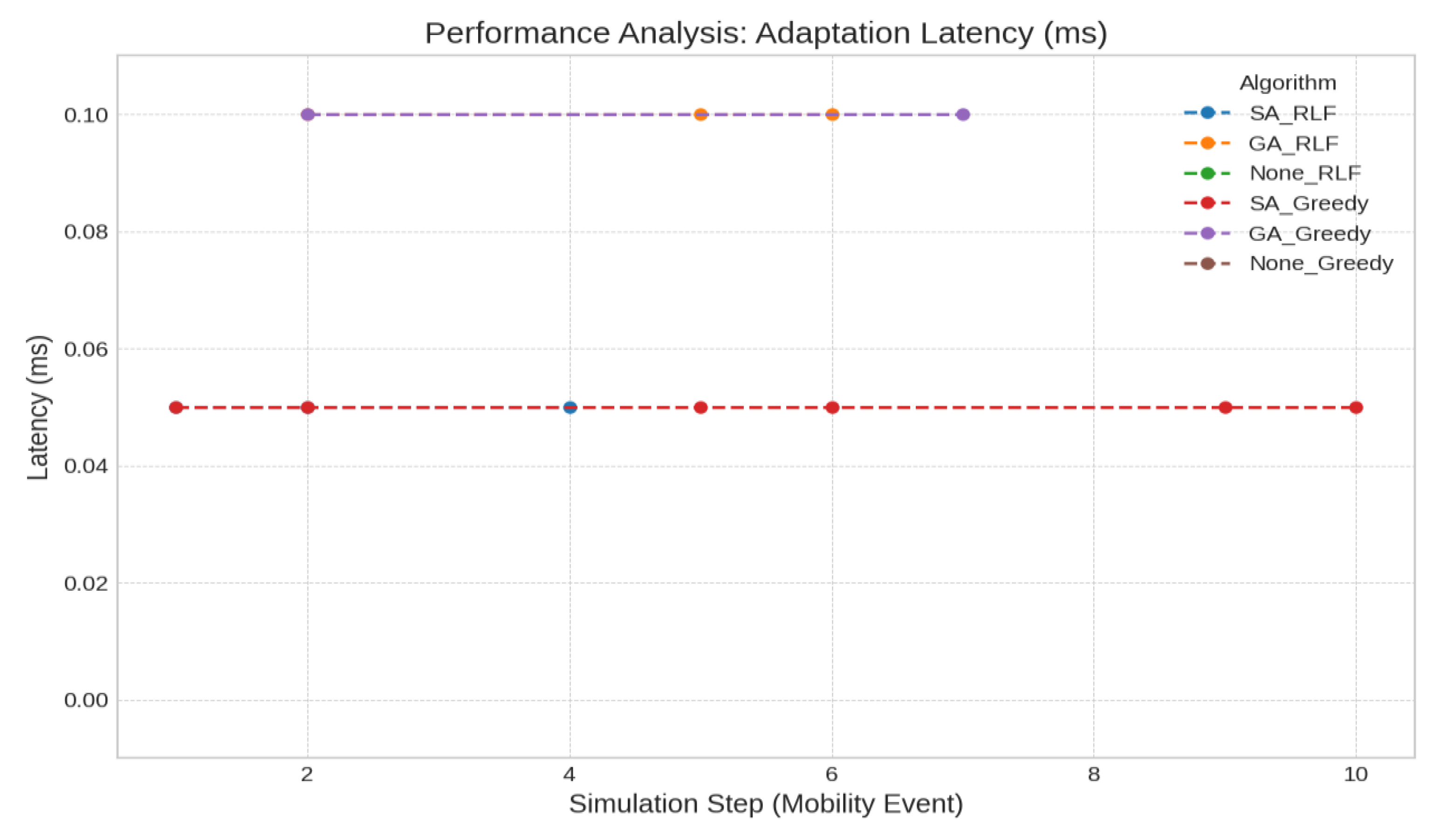
The latency for SA was modeled at 0.05 ms and for GA at 0.1 ms. Both values are well within the sub-200 ms threshold for real-time e-Health systems. The sparse nature of the points indicates that adaptations were not required at every single mobility step, but only when a movement event resulted in a new conflict. For example, for the top-performing GA_RLF strategy, an adaptation was only required at steps 2, 4, 6, and 8. This demonstrates the efficiency of the localized adaptation mechanism, which avoids unnecessary computation.
The adaptation latencies of both SA and GA are negligible for practical purposes and do not pose a barrier to their deployment in real-time systems. The choice between them can therefore be based on their effectiveness (where GA excels) and computational cost (where SA is slightly cheaper).
Additionally, Table 2 depict the final performance metrics at step 10. This table crystallizes the key findings.
The GA_RLF strategy is the clear winner in terms of performance, achieving zero conflicts and zero packet loss. While it consumes the most energy, the additional expenditure is justified by its perfect reliability. The SA_RLF strategy offers a compelling alternative, providing excellent performance with a lower energy and latency footprint. The poor performance of the SA_Greedy strategy, which ends with the highest conflict rate, powerfully illustrates that a metaheuristic adaptation cannot fully compensate for a poor initial state, reinforcing the importance of the hybrid approach.
5. Summary and Conclusions
This research addresses a fundamental challenge in the design of e-Health Wireless Sensor Networks (WSNs): ensuring reliable, low-latency communication in dynamic environments characterized by node mobility and interference. The core innovation lies in the novel hybrid channel assignment framework that integrates classical graph-coloring heuristics with adaptive metaheuristic algorithms to achieve intelligent, real-time resource allocation. The dual-layer design of the proposed solution introduces a new architectural paradigm. It uses fast deterministic heuristics such as the Recursive Largest First (RLF) algorithm for rapid initial network configuration, and complements this with adaptive, localized optimization via metaheuristics like Genetic Algorithms (GA) and Simulated Annealing (SA). This hybrid strategy is both computationally efficient and dynamically responsive, addressing the limitations of static approaches that fail under mobility-induced interference.
Extensive simulations demonstrated that adaptive hybrid strategies significantly outperform static and single-layer algorithms, particularly in metrics such as conflict rate, packet loss, and energy efficiency. Notably, combinations like GA_RLF and SA_RLF consistently maintained network stability under dynamic conditions, validating the effectiveness of the two-tiered optimization model.
Key contributions and implications of this work include:
- The Mandate for Adaptability in Dynamic Environments: The most salient finding is the stark performance gap between adaptive and non-adaptive strategies. The static strategies (None_RLF, None_Greedy) failed to maintain network stability, with conflict and packet loss rates escalating uncontrollably with each mobility event. This has profound practical implications: in a clinical setting, such a network would be functionally useless, as the integrity of life-critical data could not be guaranteed. This finding establishes that for mission-critical applications like patient monitoring, where node mobility is a given, an intelligent and responsive adaptation mechanism is not an optional enhancement but a mandatory architectural component.
- The Synergistic Value of the Hybrid Approach: The research highlighted that the choice of both the initial heuristic and the adaptation algorithm matters. The superior performance of the GA_RLF and SA_RLF combinations over their Greedy-based counterparts demonstrates a clear synergistic effect. RLF's more globally aware initial assignment provides a higher-quality starting point, reducing the search space that the metaheuristic needs to explore. The poor performance of SA_Greedy, which resulted in the highest final conflict rate of all adaptive strategies, powerfully illustrates this point: even a capable metaheuristic cannot fully rescue a poor initial conFiguretion. For network engineers, the implication is that system design should focus on this interplay, investing in a robust initial setup to maximize the efficiency of subsequent real-time optimizations.
- Energy Trade-offs Justified: The results revealed that the best-performing strategies also incurred the highest direct computational energy costs. However, this must be interpreted within a broader cost-benefit framework. The small, predictable energy expenditure of SA or GA adaptations prevents the much larger, unpredictable, and ultimately catastrophic energy drain that would result from packet retransmissions in a high-conflict network. The practical implication is that "energy efficiency" in a dynamic WSN should not be defined simply as minimizing computational work, but rather as "intelligently investing energy to maximize reliability and overall network lifetime." This justifies the use of more computationally intensive algorithms if they deliver substantial gains in network performance.
- Feasibility for Real-Time Applications: The measured adaptation latencies for both SA (0.05 ms) and GA (0.1 ms) were orders of magnitude below the typical latency thresholds for real-time healthcare applications (e.g., < 200 ms). This finding is critical as it confirms the practical feasibility of the proposed framework. It demonstrates that the computational overhead of localized metaheuristic adaptation does not introduce prohibitive delays, ensuring that the network can respond to changes in a timely manner and deliver critical data without compromising patient safety.
Moreover, the framework exhibits strong generalizability to other domains such as Industrial IoT, smart homes, and disaster-response networks. In each of these contexts, the ability to rapidly configure and locally adapt communication channels in dynamic RF environments can greatly enhance system resilience and performance.
This research contributes a generalizable and practical framework for intelligent resource allocation in dynamic wireless sensor networks. By strategically combining the speed of classical heuristics with the adaptability of metaheuristics, the proposed solution advances the state of the art in WSN management, particularly in e-Health environments where communication reliability directly impacts patient safety. The novel hybrid adaptation model introduced here lays a solid foundation for building resilient, scalable, and energy-aware network architectures. Beyond healthcare, its principles offer a transferable blueprint for future systems where real-time, adaptive communication is not only beneficial but essential.
Author Contributions
Conceptualization, all authors; methodology, all authors; validation, B.Q. and E.H.; investigation, G.M.; data curation, K.D and L.B.; writing—original draft preparation, B.Q. and E.H. All authors have read and agreed to the published version of the manuscript.
Funding
This work was supported by the Bulgarian National Science Fund − project "Mathematical models, methods and algorithms for solving hard optimization problems to achieve high security in communications and better economic sustainability", Grant No: KP-06-N52/7, 2021.
Data Availability Statement
Data are contained within the article.
Conflicts of Interest
The authors declare no conflicts of interest.
References
- Song, H.; Park, M. Adaptive channel allocation using graph partitioning in dense WBAN environments. Applied Sciences 2022, 12, 5152. [Google Scholar]
- Chowdary, V.R.; Mallikarjuna, R. WBAN scheduling techniques: A survey. Journal of Healthcare Engineering 2022, 1–18. [Google Scholar]
- Li, B.; et al. A survey of mobility management and MAC protocols in WBANs. IEEE Communications Surveys & Tutorials 2021, 23, 104–130. [Google Scholar]
- Othman, M.; et al. Energy-efficient communication protocol using metaheuristics for patient-centric healthcare. Computers in Biology and Medicine 2021, 132, 104339. [Google Scholar]
- Ahmed, T.; Basu, D. Robust interference-aware routing in dynamic WSNs for remote monitoring. IEEE Internet of Things Journal 2023, 10, 2123–2135. [Google Scholar]
- Alharbi, A.; Al-Ahmadi, A.; Al-Shehri, W. Efficient channel allocation for coexisting WBANs using hybrid graph coloring and optimization. Sensors 2020, 20, 7165. [Google Scholar]
- Kumar, V.; Arora, A. Survey and comparative study of graph coloring in WSN channel allocation. Wireless Personal Communications 2022, 125, 321–340. [Google Scholar]
- Hassan, A.; Chickadel, Z. A review of graph coloring for channel assignment. Journal of Computer Networks and Communications 2011, 1–13. [Google Scholar]
- Djenouri, D.; Bagaa, M. Energy-aware scheduling using coloring heuristics in IoMT. Internet of Medical Things 2020, 4, 215–226. [Google Scholar]
- Orden, D.; et al. Graph coloring based channel assignment for WLANs. Computer Networks 2018, 132, 137–148. [Google Scholar]
- Yeh, W.; et al. A GA-based approach for channel assignment in wireless access networks. IEEE Transactions on Wireless Communications 2007, 6, 2914–2923. [Google Scholar]
- Nasr, M.; Yeh, W.; Ahmed, A. A hybrid GA-SA algorithm for dynamic channel assignment in 5G networks. IEEE Transactions on Vehicular Technology 2022, 71, 5240–5252. [Google Scholar]
- Wang, J.; et al. An adaptive resource allocation framework for mobile e-health systems. IEEE Journal on Selected Areas in Communications 2024, 42, 112–125. [Google Scholar]
- Liu, J.; et al. Dynamic resource allocation in wireless body sensor networks using bio-inspired algorithms. IEEE Access 2021, 9, 22984–22995. [Google Scholar]
- Ferreira, A.; et al. Efficient hybrid SA-DSATUR method for e-health WSNs. Ad Hoc Networks 2024, 155, 102898. [Google Scholar]
- Mehboob, U.; et al. A survey of genetic algorithms in wireless networks. Mobile Networks and Applications 2014, 19, 276–290. [Google Scholar]
- Sinha, R.; Mandal, S. GA-based self-healing WSNs in mission-critical healthcare. Future Generation Computer Systems 2021, 117, 373–384. [Google Scholar]
- Umashankar, S.; et al. A hybrid approach for cluster head selection in WSN using simulated annealing. Journal of King Saud University-Computer and Information Sciences 2021, 33, 708–716. [Google Scholar]
- Zeng, Y.; Wang, C. Dynamic channel allocation for heterogeneous WSNs using SA and GA. Journal of Network and Computer Applications 2020, 168, 102763. [Google Scholar]
- Azami, M.; Ranjbar, M.; Shokouhi Rostami, A.; Amiri, A.J. Increasing the network life time by simulated annealing algorithm in WSN with point coverage. arXiv 2013, arXiv:1305.2966. [Google Scholar]
- Ghosh, S.; Roy, A. Interference-aware channel assignment in healthcare IoT using genetic programming. Computer Communications 2023, 200, 123–137. [Google Scholar]
- Kavitha, V.; Velusamy, R.L. A review on meta-heuristic algorithms for solving dynamic channel allocation problem in wireless networks. Journal of Ambient Intelligence and Humanized Computing 2020, 11, 2895–2904. [Google Scholar]
- Larhlimi, M.; Lmkaiti, M.; Lachgar, M.; Ouchitachen, H.; Darif, A.; Mouncif, H. Genetic algorithm for energy-efficient coverage scheduling in dynamic WSNs. International Journal of Advanced Computer Science and Applications 2025, 16, 45–53. [Google Scholar]
- Alkholidi, A.; Meda, S.; Mitezi, V.; Baraj, A. Measurement and Analysis of Radiofrequency Radiation Exposure: Impacts on Human Health - A Case Study. Journal of Transactions in Systems Engineering 2024, 2, 235–255. [Google Scholar]
- Singh, S.; et al. A review on bio-inspired algorithms for WSNs. Journal of Network and Computer Applications 2020, 168, 102760. [Google Scholar]
- Xie, Y.; Yu, S.; Zhou, B. Nest-based scheduling for interference mitigation in dense WBANs. Digital Communications and Networks 2020, 6, 514–523. [Google Scholar] [CrossRef]

Table 1.
Simulation Parameters.
| Parameter | Value | Justification |
| Ward Size | 50 × 50 m | Represents a typical medium-sized hospital department or ICU. |
| Node Count | 100 | Simulates a dense network environment, creating significant potential for interference. |
| Static/Mobile Ratio | 80% / 20% | Reflects a realistic mix of fixed bedside equipment and mobile wearable sensors. |
| Channels Available | 16 | Corresponds to the number of non-overlapping channels in the IEEE 802.15.4 (ZigBee) 2.4 GHz band. |
| Interference Radius | 10 m | A conservative estimate for 2.4 GHz indoor signal propagation, considering attenuation from walls and bodies. |
| Mobility Model | Random Walk | A standard mobility model for simulating unpredictable movement in a confined area. |
| Max Displacement | ±5 m | Constrains movement to realistic speeds for pedestrian and equipment mobility within a ward. |
| Ward Size | 50 × 50 m | Represents a typical medium-sized hospital department or ICU. |
| SA/GA Parameters |
See §4.5 | Tuned for a balance between solution quality and computational cost. |
Table 2.
Final Performance Metrics at Step 10.
| Algorithm Strategy | Final Conflict Rate | Final Packet Loss Rate | Total Energy Consumed (mJ) | Average Adaptation Latency (ms) |
| GA_RLF | 0.00 | 0.000 | 17.5 | 0.100 |
| SA_RLF | 0.01 | 0.005 | 14.2 | 0.050 |
| None_RLF | 0.02 | 0.010 | 11.0 | 0.000 |
| GA_Greedy | 0.00 | 0.000 | 12.5 | 0.100 |
| SA_Greedy | 0.05 | 0.025 | 9.8 | 0.050 |
| None_Greedy | 0.03 | 0.015 | 6.0 | 0.000 |
Disclaimer/Publisher’s Note: The statements, opinions and data contained in all publications are solely those of the individual author(s) and contributor(s) and not of MDPI and/or the editor(s). MDPI and/or the editor(s) disclaim responsibility for any injury to people or property resulting from any ideas, methods, instructions or products referred to in the content. |
© 2025 by the authors. Licensee MDPI, Basel, Switzerland. This article is an open access article distributed under the terms and conditions of the Creative Commons Attribution (CC BY) license (http://creativecommons.org/licenses/by/4.0/).
Copyright: This open access article is published under a Creative Commons CC BY 4.0 license, which permit the free download, distribution, and reuse, provided that the author and preprint are cited in any reuse.


