
Submitted:
07 July 2025
Posted:
09 July 2025
You are already at the latest version
Abstract
This paper introduces a cognitively inspired approach to word representation called step-wise approximation of embeddings, which bridges the gap between static word embeddings and fully contextualized language model outputs. Traditional embedding models like Word2Vec assign a single vector to each word, failing to account for polysemy and context-dependent meanings. In contrast, large language models produce distinct embeddings for every token instance but at the cost of interpretability and computational efficiency. We propose modeling embeddings as piecewise-constant approximations that evolve in discrete semantic steps across contexts. This approach enables a word to be represented by a finite set of context-sensitive vectors, capturing different senses or usage patterns. We formalize the approximation process using entropy-minimizing segmentation and demonstrate its application in a continuous Word2Vec setting that handles context shifts smoothly. Our experiments show that this method improves representation quality for tail entities—words with limited training frequency—yielding up to 5% improvement in question answering tasks within a retrieval-augmented generation (RAG) framework. These results suggest that step-wise approximation offers a computationally efficient and interpretable alternative to contextual embeddings, with particular benefits for underrepresented vocabulary.
Keywords:
step-wise embedding approximation
; contextual word representations
; polysemy in word embeddings
1. Introduction
The distributional hypothesis, which states that words with similar meanings tend to occur in similar linguistic contexts, constitutes a fundamental theoretical underpinning of contemporary word embedding techniques in natural language processing (NLP). This hypothesis embodies the principle that semantic similarity is correlated with contextual distribution, and finds its earliest philosophical articulation in Wittgenstein’s Philosophical Investigations (Malcolm 1954), where he asserted that “the meaning of a word is its use in the language.” Wittgenstein’s use-based view of meaning marked a significant departure from referential theories, emphasizing the functional role of language in practice.
The distributional hypothesis was subsequently formalized within linguistics during the mid-twentieth century, most notably by Zellig S. Harris, who introduced the idea of analyzing language through distributional structures (De Santis et al. 2024), and by J. R. Firth, whose slogan “You shall know a word by the company it keeps”—encapsulated the core of distributional semantics. These foundational insights provided the conceptual scaffolding for data-driven approaches to meaning representation.
In modern computational linguistics, these theoretical principles are operationalized through embedding models, which map words into continuous vector spaces based on co-occurrence statistics within large corpora. Such models, including Word2Vec, GloVe, and more recent contextual embeddings like BERT, aim to capture semantic and syntactic regularities by modeling the distributional properties of language. Moreover, these models are often integrated with the principle of compositionality, which asserts that the meaning of a complex expression is determined by the meanings of its constituents and the structural rules governing their combination.
Thus, state-of-the-art deep learning architectures in NLP are grounded in the confluence of two key linguistic traditions: the empirical, corpus-based methodology of distributional semantics, and the formal, rule-based tradition of compositional semantics. This theoretical synergy enables the development of robust models capable of representing meaning at multiple levels of granularity, from individual words to complex discourse structures.
At the core of these models lies the concept of embedding—the mapping of discrete linguistic units such as words, phrases, or even entire documents into continuous vector spaces. These embeddings are learned from vast corpora, capturing nuanced patterns of co-occurrence and semantic relatedness. Word embeddings, for instance, reflect the distributional hypothesis: words appearing in similar contexts tend to have similar meanings. More advanced techniques, such as contextual embeddings produced by Transformer-based models, go further by allowing representations to adapt dynamically depending on surrounding linguistic context. This process distills high-dimensional language usage into compact, information-rich representations that form the input to deeper neural architectures for downstream tasks.
One popular method for generating word embeddings is Word2Vec, which is based on the distributional hypothesis: words that appear in similar contexts tend to have similar meanings. Word2Vec learns word embeddings by training a neural network model to predict the context words given a target word (continuous bag of words) or predict the target word given context words (skip-gram) from a large corpus of text. Once trained, the hidden layer of the neural network serves as the word embeddings. These embeddings can then be used to represent the meaning of words in downstream NLP tasks such as sentiment analysis, machine translation, and named entity recognition.
Another approach is GloVe (Global Vectors for Word Representation), which learns word embeddings by factorizing the co-occurrence matrix of words in a corpus. GloVe captures the global statistical information of word co-occurrences and produces word embeddings that are effective in capturing semantic relationships between words.
More recently, transformer-based models like BERT (Bidirectional Encoder Representations from Transformers) and GPT (Generative Pre-trained Transformer) have gained popularity for generating contextualized word embeddings. These models use attention mechanisms to capture the context of each word in a sentence and generate word embeddings that are sensitive to the surrounding context. Representing the meaning of a word by a discrete numerical function involves learning word embeddings that capture semantic relationships between words in a continuous vector space. This allows NLP models to effectively understand and process natural language text.
However, the reliance on embeddings can inadvertently introduce hallucinations, particularly for tail data—that is, rare or underrepresented entities, expressions, or combinations not sufficiently captured during training. Since embedding spaces are shaped by the statistical properties of the training corpus, tail items may receive poor or ambiguous representations. Consequently, when models encounter these items, they may interpolate their meaning from nearby but semantically inappropriate vectors, leading to confident but inaccurate outputs. In generative tasks, this manifests as hallucinations—fabricated or incorrect information not supported by the input or real-world knowledge—emerging from the model’s attempt to generalize beyond its data support.
To address noise and inaccuracies in embeddings, especially those generated by simpler models like Continuous Bag of Words (CBOW) (Mikolov et al., 2013), step-wise approximation can be used to refine these embeddings progressively (Figure 1). CBOW generates word embeddings by predicting a target word from the surrounding context words, averaging their vectors to produce a single representation. While efficient, this averaging process can introduce noise by blending diverse contexts indiscriminately, which reduces the precision of the resulting embedding (Levy & Goldberg, 2014; Ethayarajh, 2019).
Step-wise approximation tackles this issue by decomposing the embedding process into multiple stages instead of producing a final embedding in one step (Liang et al., 2019). Rather than directly averaging all context vectors at once, the model applies a sequence of functions that iteratively refine the representation, selectively weighting or transforming context words based on their relevance (Coenen et al., 2019). For example, early steps may emphasize the most informative context words, while later steps reduce the impact of noisy or less relevant signals.
This gradual refinement helps filter out noise that would otherwise be embedded through blunt averaging, allowing the model to generate cleaner, more context-sensitive embeddings. By approximating the CBOW process as a step-wise function, the model gains greater control over how context contributes to the final vector, improving robustness and accuracy, especially for ambiguous or rare words where noise can disproportionately degrade the embedding quality (Murphy et al., 2012; Jia & Liang, 2017).
Recent research has shown that hallucinations in language models—where models generate factually incorrect or contextually unsupported outputs—are often exacerbated by noisy or imprecise semantic representations. In this context, applying step-wise approximation to embedding generation, such as in modified versions of the CBOW model, can significantly reduce hallucinatory behavior by refining contextual representations iteratively. Instead of collapsing all context vectors into a single averaged representation upfront, step-wise methods progressively adjust the influence of each word based on its relevance and coherence with the target word. This selective weighting prevents misleading signals from dominating the final embedding, especially in ambiguous or low-resource contexts where noise is more likely to distort meaning. By enabling a more nuanced construction of semantic vectors, step-wise approaches enhance the fidelity of internal representations, which in turn leads to more accurate and grounded language generation (Coenen et al. 2019).
1.1. From Discrete to Step-Wise Embeddings
Discrete embedding-based language models, such as Word2Vec (Mikolov et al., 2013), DRG2Vec (Shu et al., 2020), Dict2Vec (Tissier et al., 2017) utilize structured sources like Wikipedia or dictionaries as the input corpus. These models apply a sliding context window along the input text and optimize a similarity-based objective, typically maximizing the co-occurrence likelihood of words within a fixed window size. Upon training completion, each word is assigned a single, discrete embedding vector, which can then be used directly during downstream inference tasks.
However, this approach assigns one static vector per word (or token), which limits the ability of the model to capture context-specific nuances, especially for polysemous words—those with multiple meanings depending on context (e.g., the word “bank” can refer to either a financial institution or the side of a river). Because the embeddings are fixed after training, these models often blur or average the semantic representations across all senses of a word, which degrades performance in tasks that require fine-grained semantic distinctions.
To address this limitation, in this chapter we explore the step-wise approximation of embeddings, an approach that introduces piecewise representations of words based on their contextual semantics. Instead of associating each word with a single fixed vector, step-wise approximation represents a word as a set of discrete semantic steps, where each step approximates a distinct contextual meaning. These steps can be learned by partitioning the training data into clusters of contexts (e.g., via k-means or attention-based segmentation) and assigning different sub-vectors or embeddings to each partition. The result is a multi-faceted embedding where a word like “bank” is represented by a small set of contextually grounded vectors, one for financial uses, another for geographic references, and so on.
While language models rely on continuous contextual embeddings, which allow for an infinite number of representations for each token, it contrasts with the way humans perceive language, where each word often carries only a limited number of distinct senses. For example, consider the visualization of the different contextual embeddings of the word “draft” in Figure 2.
t-SNE is a t-distributed stochastic neighbor embedding, introduced by van der Maaten and Geoffrey Hinton in (2008), a popular dimensionality reduction technique used for visualizing high-dimensional data in 2D. Unlike methods like PCA, which preserve global variance, t-SNE focuses on preserving local similarities (i.e., nearby points in high-dimensional space stay close in 2D. We can observe a good amount of variation in the embeddings, but there are only two main senses. as a noun and as a verb.
Unlike LLMs which learn language by processing massive corpora and generating highly context-dependent embeddings for each token, human language acquisition follows a more incremental and discrete process. When we learn a new word, we typically store a limited set of senses, each associated with distinct contextual patterns, and retrieve the appropriate meaning as needed based on surrounding cues (Davis & Gaskell, 2009; Wojcik, 2013). This cognitive strategy suggests an alternative to the LLM paradigm: rather than generating a unique embedding for every possible context, could we instead approximate meaning using a finite set of step-wise approximations of embeddings, each representing a distinct semantic variant? Such an approach would mirror human-like understanding more closely, offering interpretable and computationally efficient representations while still capturing key contextual variations.
1.2. Step-Wise Approximation of Continuous Bag of Words
Continuous bag of words (CBOW) predicts a word from a context using a softmax over the entire vocabulary. We have a probability distribution
, (1)
where: is the output vector for the target word, h is the average of the context word vectors, V is the vocabulary (can be millions of words). We intend to approximate the P(wt) by means of approximation function Ps(wt). This approximation function Ps(wt) is fully determined by P(wt) it approximates, and specific words (values) wi, where it jumps from P(wi) to P(wi+1). The values for wi are to be determined (Figure 3)
Instead of expressing a meaning of a word via the totality of other words in V, we do that in the basis of classes of equivalent words where the distribution Ps(wt) is constant (forms a step).
1.3. Minimization of Entropy Production and CBOW
In thermodynamics, there are two classes of problems where the criterion is the minimization of entropy production (Berry et al. 2020. One such class considers processes with a fixed duration and a given average flow of energy or matter. The goal is to find the law of evolution for the intensive variables (such as temperature or chemical potential) of the subsystems participating in the exchange, such that total entropy production is minimized. These are known as minimum dissipation processes.
The CBOW model can be viewed as an information-theoretic analog of such thermodynamic systems. The correspondence maps out in the following way (Table 1).
In minimum dissipation thermodynamic problems, the system evolves along the trajectory x(t) that minimizes the total entropy production over time:
This can be mirrored in CBOW as optimization objective (Information-Theoretic Form): CBOW minimizes the cross-entropy between the true word distribution and the predicted distribution from the context:
subject to constraints on embedding norm or training time
Where:
- c: context window (sum/avg of embeddings)
- w: center word
- θ: parameters of embeddings
- : softmax output
Interpretation as minimum entropy production is as follows. During training, the embedding vectors vw evolve via gradient flow, analogous to the evolution of physical variables xi(t). The objective functional being minimized is cross-entropy, which corresponds to informational entropy production. The learning process seeks an embedding configuration where information is stored efficiently (low entropy state), under constraints (context size, training steps).
Thus, CBOW learning is akin to finding a minimum-dissipation path in parameter space, subject to fixed information flow and temporal limits. Hence CBOW can be interpreted as an information-dynamic system analogous to minimum entropy production problems in thermodynamics (Figure 4):
- Both minimize a cumulative cost over time (entropy vs. loss).
- Both evolve under constraints (physical flows vs. learning limits).
- The optimal embeddings in CBOW correspond to steady states of minimal informational dissipation, much like how thermodynamic systems evolve to minimize physical dissipation.
The paper is organized as follows. We begin by motivating the transition from discrete to step-wise embeddings, and introduce a mathematical formulation for approximating continuous semantic evolution using entropy-minimizing segmentation. We then explore how continuous Word2Vec models can be extended to handle context shifts more robustly through step-wise embedding updates. Next, we detail practical methods for computing and modeling step-wise embeddings, and demonstrate their application in a setting of enhancing embedding robustness under hallucination-inducing conditions.
To evaluate the proposed method, we assess its relevance in a retrieval-augmented generation framework, focusing on tail entities, where standard LLM embeddings often degrade in quality. Our experiments show that step-wise approximation improves performance for rare words while maintaining competitiveness for frequent ones.
Overall, this work contributes a scalable, cognitively inspired alternative to continuous context-based embeddings, enabling more interpretable and adaptable representations for a wide range of NLP tasks.
2. Continuous word2vec and Word Profiles
Representing the meaning of a word by a continuous function is a fundamental concept in NLP known as word embedding. In NLP, text embeddings (e.g., word embeddings, sentence embeddings) are used to represent textual data in a continuous vector space. Word embeddings are dense vector representations of words in a vector space, where each dimension of the vector captures different aspects of the word’s meaning.
To form a continuous word embedding, we need to form a basis to express a meaning of words (Galitsky 2025). To express a meaning of a noun, we build its profile in the basis of verbs applicable to this noun. Analogously, to express a meaning of a verb, we build its profile in the basis of nouns this verb is acting upon. To have the basis for verbs fixed in the most general form, we select the noun with a broad scope like human or animal. Then we select a spectrum of verbs related to, for example, physical or mental activity of humans. To form a basis for human, we order the verbs according to the distance to human, from the most “similar” to least “similar”. Another option for basis construction is to start with a most general verb like ‘move’ and finish the basis with a specific movement verb like jump. The basis for verbs is formed in a similar manner.
A profile for a word is a sequence of distances to the elements of the basis. For most general and representative words like human – {move, walk, sit, hike, jump} a typical profile is a monotonic decreasing function. What makes this function continuous is that the elements of the basis have “intermediate” meanings in between, corresponding to “fictitious” words positioned “in between” the meanings of the words of the basis. The range [walk…sit] is filled with [mostly walk and sit sometimes, …, mostly sit and sometimes stand up and walk] meaning values. Hence the values between the basis can be interpolated in a continuous manner. Although there is no specific word to express this intermediate position in the basis, the respective meaning can be expressed by a natural language phrase. Hence the profile is a continuous function, close to monotonic for a broad, general, canonic nouns and verbs and non-monotonic for other, specific nouns and verbs. Other parts of speech such as adjectives can have this basis as nouns, or verb phrases including nouns.
A verb-noun word2vec distance matrix is shown in Figure 5. As a simple case, we formed a list of verbs and corresponding nouns such as run-runner. The verbs are ordered by a distance to the head verb: we start with the lowest distance and end with the highest distance for verbs in a given semantic family of verbs for movement types.
Then for each noun we form a profile of distances {|embed(run)-embed(running)|, |embed(jump)-embed(running)|, … |embed(jump)-embed(running)|}. The curve is continuous as we can form a fuzzy meaning 30% run and 70% jump.
Once individual words are encoded as profiles, a phrase from these words is encoded as a concatenation of the profiles for individual words. This concatenation is not a continuous function any more, and similarity of each profile needs to be computed separately.
A continuous Word2Vec embedding is a real-valued vector representation of a word, learned from text using neural language models, where semantic similarity is preserved as geometric proximity in the embedding space.
If the vocabulary size is V and embedding size is D, then the embedding matrix E∈RV×D maps each word wi to a vector v⃗i ∈ RD, CBOW and Skip-Gram models learn the matrix E by minimizing prediction error:
- Skip-Gram: Predict context words from a target word.
- CBOW: Predict the target word from surrounding context words.
3. Step-Wise Approximation of Text Embeddings
Step-wise approximation refers to breaking down the embedding process into discrete steps or stages, often using piecewise-constant functions. This approach simplifies complex embeddings by approximating them with simpler, step-like functions.
When the context of the text changes (e.g., shifting from one topic to another), the step-wise approximation may fail to capture the nuances of the new context. This can lead to hallucinations , where the model generates incorrect or nonsensical outputs because it misinterprets the context or fails to adapt smoothly to the change.
The challenge lies in ensuring that the step-wise approximation remains accurate even as the context changes. If the approximation is too coarse or poorly aligned with the underlying semantics, it can introduce errors that propagate through the system.
3.1. Why Step-Wise Approximation is Needed in CBOW
Computing this denominator (the normalization term) is too expensive for large vocabularies — it requires computing scores for every single word in the vocabulary on every training step. To solve this problem, instead of computing probabilities over the entire vocabulary, CBOW just learns to distinguish the correct word from a few “negative” words. For each training example, we form positive pair: (context → true target word) and negative samples: (context → random, unrelated words). The objective of CBOW is to maximize the probability of a target word given its context words:
.
here σ is the sigmoid function and k is number of negative samples (e.g., 5–20)
Hierarchical softmax replaces the flat softmax with a binary tree over the vocabulary. Each word is a leaf node; predicting a word involves walking down the tree. Instead of computing |V| scores, we compute log₂|V| scores. This is useful when you want to retain probability estimates.
Subsampling of frequent words (is not softmax-related but improves efficiency. Very frequent words (like “the”, “is”) are randomly dropped to speed up training and reduce their dominance. Step-wise approximation is essential in CBOW to avoid computing full softmax over large vocabularies. It is implemented through techniques like negative sampling or hierarchical softmax, which drastically reduce computation while still enabling effective learning of word embeddings.
CBOW and skip-gram both produce dense and low-dimensional word vector representations that can be used to solve diversified Natural Language Processing challenges. These approaches produce vectors with a significant flaw: they only have local word co-occurrence information and no global co-occurrence information. Local and global information are merged as input to a two-layer neural network (Huang et al. 2012).
Graph embedding is employed to combine local and global co-occurrence counts. The nodes in the graph represent words, and the weight of each edge is determined by a combination of local and global co-occurrence counts. When compared to word2vec and GloVe, the graph embedding outperforms sequence baseline in terms of word similarity. Since the GloVe model was created to address the constraints of word2vec. Moreover, clustering is applied in the context of a word, where the word sense is represented by the centroid of each cluster (Reisinger and Mooney 2010) Multi-prototype vector-space models of word meaning. The original word2vec model is also extended for producing multi-sense word embeddings (Wang et al. 2025).
3.2. Identifying Breakpoints for Context Changes
In the context of text embeddings, breakpoints (ti) can correspond to points where the context changes significantly. For example:
- A change in topic (e.g., moving from discussing “climate change” to “technology”).
- A shift in tone or sentiment (e.g., from positive to negative).
- A transition between different types of information (e.g., factual vs. speculative).
To identify these breakpoints one can use context-aware models (e.g., transformers) to detect shifts in semantic meaning. It is also possible to apply change-point detection algorithms to analyze the embedding vectors and identify points where the distribution of embeddings changes abruptly.
We minimize the difference between the original function x(t) and the approximated function xs(t). In the context of text embeddings:
- Original Function x(t): The true, continuous representation of the text embedding over time or sequence.
- Approximated Function xs(t): The step-wise approximation of the embedding.
To minimize the error, one can use metric-based criteria to evaluate the quality of the approximation. Common metrics include:
- Euclidean distance between the original and approximated embeddings.
- Cosine similarity to measure the alignment of embedding vectors.
- Mean Squared Error (MSE) to quantify the overall discrepancy.
We need to ensure that the choice of breakpoints (ti) minimizes the cumulative error across all intervals ([ti−1,ti]).
3.3. Handling Context Changes Smoothly
The choice of ti affects only the preceding and following intervals. This suggests a localized approach to handling context changes:
- Adaptive step size: adjust the granularity of the step-wise approximation dynamically. For example, use finer steps during rapid context changes and coarser steps during stable contexts.
- Interpolation: instead of purely step-wise approximation, one can consider using interpolation techniques (e.g., linear or spline interpolation) to smooth transitions between breakpoints.
In NLP, one introduces intermediate embeddings that bridge the gap between two distinct contexts. These intermediate embeddings can help the model adapt smoothly to context changes without generating hallucinations. This is done use contextualized embeddings (e.g., BERT, RoBERTa) that are pre-trained to handle context-dependent meanings.
There is an iterative process to refine the approximation by minimizing the sum of differences between x(t) and xs(t). To apply this principle to text embeddings, we start with an initial set of breakpoints (ti). We then evaluate the approximation using metrics like MSE or cosine similarity.
Finally, we adjust the breakpoints iteratively to reduce the error, focusing on regions where context changes occur. The steps are as follows:
- Detect context changes, using advanced NLP techniques (e.g., attention mechanisms, change-point detection) to identify points where the context shifts.
- Refine step-wise Approximation, choosing breakpoints (ti) strategically to align with context changes. We use metrics like Euclidean distance or cosine similarity to evaluate and optimize the approximation.
- Smooth transitions, introducing intermediate embeddings or using interpolation to bridge gaps between contexts. We then employ contextualized models that adapt dynamically to changing contexts.
- Iterate and validate, continuously refine the approximation by adjusting breakpoints and evaluating performance.
- Test the model on diverse datasets to ensure robustness against context changes.
The approximating function xs(t) is completely determined by the function x(t) it approximates and the values ti, at which it jumps from x(ti) to x(ti+1). The values of the “breakpoints” ti are the unknown variables in such problems (Figure 3).
The criteria used to search for these variables can vary. In approximation problems, this could be the distance between x(t) and xs(t) in some metric or uniform approximation. Since the choice of ti affects the function xs(t) only on the preceding and succeeding intervals, this choice should minimize the total difference between x(t) and xs(t) only on the interval [ti−1,t i+1]. Thus, with the introduction of each new jump point ti, the reduction in the criterion on this interval should be maximized.
We approximate a continuous embedding function x(t) using a piecewise-constant function xs(t) designed to approximate the original function x(t) using a series of constant segments xs(t) is defined by two key components:
- The original function x(t), which serves as the target for approximation.
- A set of breakpoints ti, where the approximating function xs(t) changes its value abruptly (jumps from one constant segment to another). The breakpoints ti determine where the approximating function xs(t) transitions between different constant values. In many approximation problems, the exact locations of these breakpoints (ti) are not known beforehand and must be determined as part of the solution. At each breakpoint ti, the function xs(t) jumps from x(ti) to x(ti+1), creating a step-like structure.
When the goal is to find the best set of breakpoints ti such that the approximating function xs(t) closely matches the original embedding function x(t), the possible metrics are:
- Euclidean Distance : Minimize the sum of squared differences between x(t) and xs(t).
- Maximum Error: Ensure that the maximum deviation between x(t) and xs(t) is minimized.
- Uniform Approximation : Ensure that the error between x(t) and xs(t) is evenly distributed across the entire domain.
Each breakpoint ti affects the behavior of xs(t) only on the intervals immediately before and after it, i.e., [ti-1,ti] and [ti,ti+1]. This localized impact simplifies the optimization process because the effect of ti can be analyzed independently on these two intervals.
4. Solving Step-Wise Approximation
Let we have an embedding distribution function such that there exists the integral . The derivative . We need to find breakpoints such that
The value
The condition of minimality of this value over leads to boundary value problem
Since the function and its derivatives are specified, equation (2) determines which is an optimality assertion.
4.1. Implicit Optimization Assertion
An assertion for the breakpoints can be obtained in an implicit form ; however in the case where this equality can be resolved relative to , the following conditions would hold:
- ,
- (symmetric function),
- .
The last condition states that value must be optimal not only for , but also for values, calculated in the same way and positioned between and . Functions which perform averaging of satisfy this condition including the arithmetic mean or geometric mean of these values
Example 1: Let
Then condition (2) will look like:
Here all intervals between breakpoints must be equal have value , function - среднее арифметическoе, and a minimum difference x(t) and its step-wise approximation is .
Example 2. Let
Then condition (2) will be
As a rule, the “shooting” method is used to solve such a boundary value problem (4). In this case, all other “breaking points” are set and calculated according to condition (4) up to . If it turns out that , the problem is solved. Otherwise, one sets another value of and the computation is repeated.
4.2. Computing Approximated Embedding
We express the distance between the original embedding x(t) and its step-wise approximation xs(t) as , , Let us have this distance ƞ and breakpoints and . This distance function obeys . In the interval the function , and in the interval . We need to find such that the distance between functions and in the interval between these points is minimum over . The optimality condition have the form
Then taking into account the properties of ƞ we obtain the equation for finding n approximation breakpoints
4.3. Modeling Changing Embeddings
In contrast to the traditional concept of embeddings, where each word is rep resented by a single vector, sense embeddings as sociate multiple vectors per word, where each one of the vectors aims to capture a different meaning (Camacho-Collados and Pilehvar, 2018). LMMS (Loureiro et al., 2021) generates embeddings per sense key defined by annotated resource, such as WordNet (Miller 1995). As a result, LMMS can achieve more precise representations for each sense key but lacks support for most datasets consisting of plain text. Thus chapter develops a general solution to generating multiple embeddings per token without requiring annotation and an evolution of embedding over time.
The derivation (7) about step-wise approximation of embeddings can significantly improve vector similarity search in vector databases, especially when embeddings change over time, like in contextual or dynamic systems. Most vector databases (like FAISS, Pinecone, Weaviate) use static embeddings and compute cosine or L2 distance between a query and a set of stored vectors:
q-x
However, if embeddings are evolving functions of time (or context, training steps, etc.), comparing fixed vectors may miss nuances of semantic drift or temporal smoothness.
We have defined the distance between a function x(t) (e.g., a dynamically updated embedding) and its step-wise approximation xs(t), chosen to minimize the total deviation η(x, xs) over each segment [ti−1,ti+1]. We index time-series embeddings with step-wise approximation. If embeddings x(t)∈ℝ change (e.g., based on dialogue turns, document growth, or RL training steps), we store a step-wise compressed version of the trajectory using this optimization (minimizing total distance η). In vector DB, instead of one vector per item, we store multiple segments with x(ti) representing the value over that time block. At the query-time, we match queries against all segments and interpolate.
On top of that, we use distance function η as a custom similarity. Instead of cosine or Euclidean distance, we define
(8)
This can be computed efficiently via lookup or pre-integration, and used as:
similarity(q,x)=−η(q,xs)
This distance respects temporal or semantic smoothness, and avoids sharp changes that occur in non-smooth embeddings.
Hence the compression occurs with accuracy control. The optimality condition derived (stationary condition for ti) allows us to compress dynamic embeddings adaptively. Moreover, we store fewer vectors without significantly degrading search accuracy—information-theoretic compression.
For time-evolving user embeddings in recommendation, step-wise approximation of dynamic embedding compresses and track evolving preferences. For long documents where meaning shifts over paragraphs, we use paragraph-wise anchor embeddings. Also, for LLMs with prompt-driven context change, step-wise approximation matches a query against dynamic context.
5. Improving Embedding in a Fight with Hallucination
Incorrect transformer embeddings can contribute to hallucinations in language model outputs. The possibilities of hallucinations are as follows:
- Semantic misrepresentation: if embeddings fail to capture the true meaning of a token or context (e.g., conflating “apple” the fruit with “Apple” the company), the model may draw faulty associations. This can lead to outputs that are semantically incoherent or factually wrong.
- Tokenization artifacts. Poor tokenization can yield fragmented or misleading embeddings. For example, rare or out-of-vocabulary words may get broken into subwords in a way that loses meaning. As a result, the model may generate text unrelated to the input’s intended meaning.
- Contextual drift. If the embedding layer (or early transformer layers) fail to preserve relevant context, the decoder or downstream attention layers may build on distorted input, amplifying errors into hallucinations.
- Training data bias or sparsity. Embeddings trained on biased or incomplete corpora can reflect these gaps. The model may hallucinate facts that “fit” patterns in the training data even if they aren’t real. This leads to making up citations, events, or medical facts.
For example, for input: “The president of Canada is...” incorrect embedding may overweight the term “president” and neglect the fact that Canada has a prime minister, not a president. Hallucinated output is “Justin Trudeau is the president of Canada.”
For mitigating hallucination, we could perform embedding quality control such as improving pretraining data, subword segmentation, or using supervised alignment (e.g., with grounding in knowledge bases). Post-hoc analysis would also be helpful, such as probing internal representations for semantic accuracy. However, the most efficient approach is Retrieval-Augmented Models (RAG) which reduce the reliance on embeddings alone by retrieving grounded facts. Step-wise approximation of embedding of tail words turn out to be most efficient way to prevent hallucination in underrepresented knowledge.
6. Evaluation of Relevance
We evaluate relevance improvement due to improved vector matching in RAG setting. To evaluate the relevance improvement from applying step-wise approximation to CBOW embeddings in a RAG system, one can measure the quality of retrieved documents based on their alignment with the query. In this setup, both queries and documents are encoded using the refined step-wise CBOW embeddings and stored in a vector database FAISS. The evaluation involves comparing retrieval performance metrics Normalized Discounted Cumulative Gain (NDCG), when using standard CBOW embeddings versus step-wise approximated embeddings. Specifically, if the step-wise approach improves semantic resolution by reducing noise and better modeling context, it should yield more accurate nearest-neighbor matches in the vector space, resulting in higher retrieval accuracy. Additionally, end-to-end evaluation through answer relevance scoring (e.g., using BLEU on the final generated response) provides further evidence of how enhanced vector matching translates into better contextual grounding of the generated output.
6.1. Dataset
Mallen et al. (2023) observed that popular open-domain QA datasets like Natural Questions (NQ) tend to focus on widely known entities and have varied question phrasing, making it hard to analyze relation types. To support fine-grained memorization analysis, we rely on PopQA, a large-scale entity-centric QA dataset featuring entities with diverse popularity levels.
Mallen et al. (2023) built PopQA by randomly sampling 16 types of knowledge triples from Wikidata and turning them into natural language questions using relation-specific templates. Each triple (Subject, Relation, Object) is verbalized into a question by inserting the subject into a manually created template. Valid answers are all entities linked to the subject via that relation in Wikidata. The authors verified that the approach is robust across different templates. Thanks to Wikidata grounding, PopQA supports reliable popularity and relation-type analysis. Another part of question answering dataset is formed from EntityQuestions (Sciavolino et al., 2021), a dataset designed to include both common and long-tail entities.
We use Wikipedia page views as a measure of popularity and form knowledge triples from Wikidata, varying the level of popularity. The triples have the form <subject, relationship, object> (Figure 6).
Questions are focused on the original tail entities and relationship types for which a limited context for embedding computation is available. A question answering session against this dataset produces a sequence of candidate answers so NDCG is a good measure of relevance
6.2. Assessing RAG Relevance for Tail Entities
Since embedding relevance improvements are particularly important for tail entities—those that occur infrequently—we evaluate the impact of these improvements separately for less frequent and more frequent entities. We assume that errors in answers are due to hallucinations in questions vs answer representation caused by incorrect embeddings. Specifically, we assess question answering accuracy using our RAG system based on:
5. the default embedding,
- its step-wise approximation, and
- a dynamic embedding modeled through step-wise approximation over time.
In Table 2, we compare accuracy for popular entities (popularity > 10⁵) and tail entities (popularity < 10³) across the three embedding variants. The second and third columns show baseline accuracy using the default embedding (grayed out for reference).
We observe that for tail entities, the step-wise approximation yields a 4% performance improvement, whereas for popular entities, the gain is only 2%. When modeling the evolution of the embedding using a step-wise approach, tail entities show an even larger improvement of 5%, while accuracy for popular entities slightly declines. Hence step-wise approximation improves the quality of embeddings for infrequent words and as a result boosts question answering relevance, as we observed.
7. Conclusions
In our previous study (Galitsky 2021) we subjected embedding techniques to critical evaluation and observed its limitations in expressing semantic relatedness of words. We analyzed a representation of meaning by the distributional semantics and also obtained an anecdotal evidence about various systems employing it. To overcome the revealed limitations of the traditional embedding techniques, where similarity is computed between words of different semantic roles, we proposed to use them on top of a linguistic structure, not in a stand-alone mode. In the phrase similarity assessment task, only when phrases are aligned and syntactic, semantic and entity-based map is established, we assessed word2vec similarity between aligned words. We added the distributional semantics feature to the results of syntactic, semantic and entity/attribute-based generalizations and observed an improvement in the similarity assessment task. It turned out that structurized word2vec improves the similarity assessment task performed by the integrated syntactic, abstract meaning representation and entity comparison baseline system by more than 10%.
Step-wise approximation serves as a computationally efficient alternative to fully contextual embeddings (e.g., from BERT), enabling models to disambiguate meanings with lightweight inference mechanisms. At test time, the model can match the current context to the nearest precomputed step and select the most appropriate sub-embedding. This maintains the inference efficiency of discrete models while providing a finer granularity of semantic representation.
Step-wise approximation thus bridges the gap between traditional word embeddings and modern contextual language models. It enhances the representational capacity of static embeddings without incurring the full cost of deep transformer-based encoders, making it particularly useful for applications where scalability, interpretability, or real-time inference is critical.
Our findings demonstrate that our step-wise approximation of embeddings offers clear benefits for improving semantic representations of infrequent (tail) entities. Specifically, we observed a 4% performance gain for tail entities using step-wise approximation, compared to a more modest 2% gain for popular entities. Furthermore, when modeling the evolution of embeddings through a step-wise mechanism, tail entities exhibited an even greater improvement of 5%, while performance for popular entities slightly declined. These results suggest that step-wise approximation is particularly effective at enhancing the embedding quality for less frequent terms, leading to improved relevance in downstream tasks such as question answering.
References
- Andresen B, Salamon P, Tsyrlin AM (2025) Step-wise function approximation and intermediate equilibriums in thermodynamics. Unpublished manuscript.
- Berry, R.S.; Salamon, P.; Andresen, B. How It All Began. Entropy 2020, 22, 908. [Google Scholar] [CrossRef] [PubMed]
- Camacho-Collados J and Mohammad Taher Pilehvar. 2018.From word to sense embeddings: A survey on vector representations of meaning.Journal of Artificial Intelligence Research, 63:743–788.
- Coenen A, Emily Reif, Ann Yuan, Been Kim, Adam Pearce, Fernanda Viégas, Martin Wattenberg (2019) Visualizing and Measuring the Geometry of BERT arXiv:1906.02715.
- Ethayarajh, K. (2019). How contextual are contextualized word representations? Proceedings of the 2019 Conference on Empirical Methods in Natural Language Processing and the 9th International Joint Conference on Natural Language Processing (EMNLP-IJCNLP), 1–14. [CrossRef]
- Galitsky B (2021) Distributional Semantics for CRM: MakingWord2vec Models Robust by Structurizing Them. In Artificial Intelligence for Customer Relationship Management. Springer: Cham, pp 25-56.
- Galitsky B (2025) Employing Kolmogorov–Arnold network for man–machine collaboration. In Lawless et al., editors: Bi-directionality in human-machine collaborative systems.
- Huang EH, Socher R, Manning CD, Ng AY (2012) Improve Word Representation via Global Context and Multiple Word prototypes. In: Proceedings of the 50th annual meeting of the association for computational linguistics. Islan: Korea: Association for Computational Linguistics, 873–882.
- Jia, R., & Liang, P. (2017). Adversarial examples for evaluating reading comprehension systems. Proceedings of the 2017 Conference on Empirical Methods in Natural Language Processing (EMNLP) , 2023–2033. [CrossRef]
- Levy, O., & Goldberg, Y. (2014). Neural word embedding as implicit matrix factorization. In Advances in Neural Information Processing Systems (NeurIPS) , 27, 2164–2172.
- Liang, P. , Huai, M., & Zhang, A. (2019). Word embedding refinement: A survey of theoretical and empirical techniques. ACM Transactions on Information Systems (TOIS), 37 (3), 1–40. [CrossRef]
- Malcolm N (1954) Wittgenstein’s philosophical investigations,” Philos. Rev., vol. 63, no. 4, pp. 530–559, 1954.
- Mallen A, Akari Asai, Victor Zhong, Rajarshi Das, Daniel Khashabi, Hannaneh Hajishirzi. (2022) When Not to Trust Language Models: Investigating Effectiveness of Parametric and Non-Parametric Memories arXiv:2212.10511.
- Mikolov, T. , Chen, K., Corrado, G., & Dean, J. (2013). Efficient estimation of word representations in vector space. arXiv 2013, arXiv:1301.3781. [Google Scholar]
- Murphy, B. R., Talukdar, P. P., & Crammer, K. (2012). Learning from implicitly supervised sequential data. Machine Learning, 86 (2), 197–233. [CrossRef]
- Reisinger J, Mooney RJ (2010) Multi-prototype vector-space models of word meaning. In: NAACL HLT 2010 - human language technologies: the 2010 annual conference of the North American chapter of the association for computational linguistics, proceedings of the main conference, no June, 109–117.
- Sciavolino C, Zexuan Zhong, Jinhyuk Lee, and Danqi Chen. 2021. Simple entity-centric questions challenge dense retrievers. In Proceedings of the 2021 Conference on Empirical Methods in Natural Language Processing.
- Shu X, Bowen Yu, Zhenyu Zhang, and Tingwen Liu. 2020. Drg2vec: Learning word representations from definition relational graph. In 2020 International Joint Conference on Neural Networks (IJCNN), pages 1–9. IEEE.
- Tissier J, Christophe Gravier, and Amaury Habrard (2017) Dict2vec: Learning word embeddings using lexical dictionaries. In Conference on Empirical Methods in Natural Language Processing (EMNLP 2017), pages 254–263.
- Tsirlin, A.M.; Balunov, A.I.; Sukin, I.A. Finite-Time Thermodynamics: Problems, Approaches, and Results. Entropy 2025, 27, 649. [Google Scholar] [CrossRef] [PubMed]
- Van der Maaten L, Geoffrey Hinton (2008) Visualizing Data using t-SNE. JMLR 9(86):2579−2605, 2008.
- Wang Q, Mohammed J. Zaki, Georgios Kollias, Vasileios Kalantzis (2025) Multi-Sense Embeddings for Language Models and Knowledge Distillation. arXiv:2504.06036v1.
Figure 1.
Our approach to word embedding where step-wise approximation is beneficial.
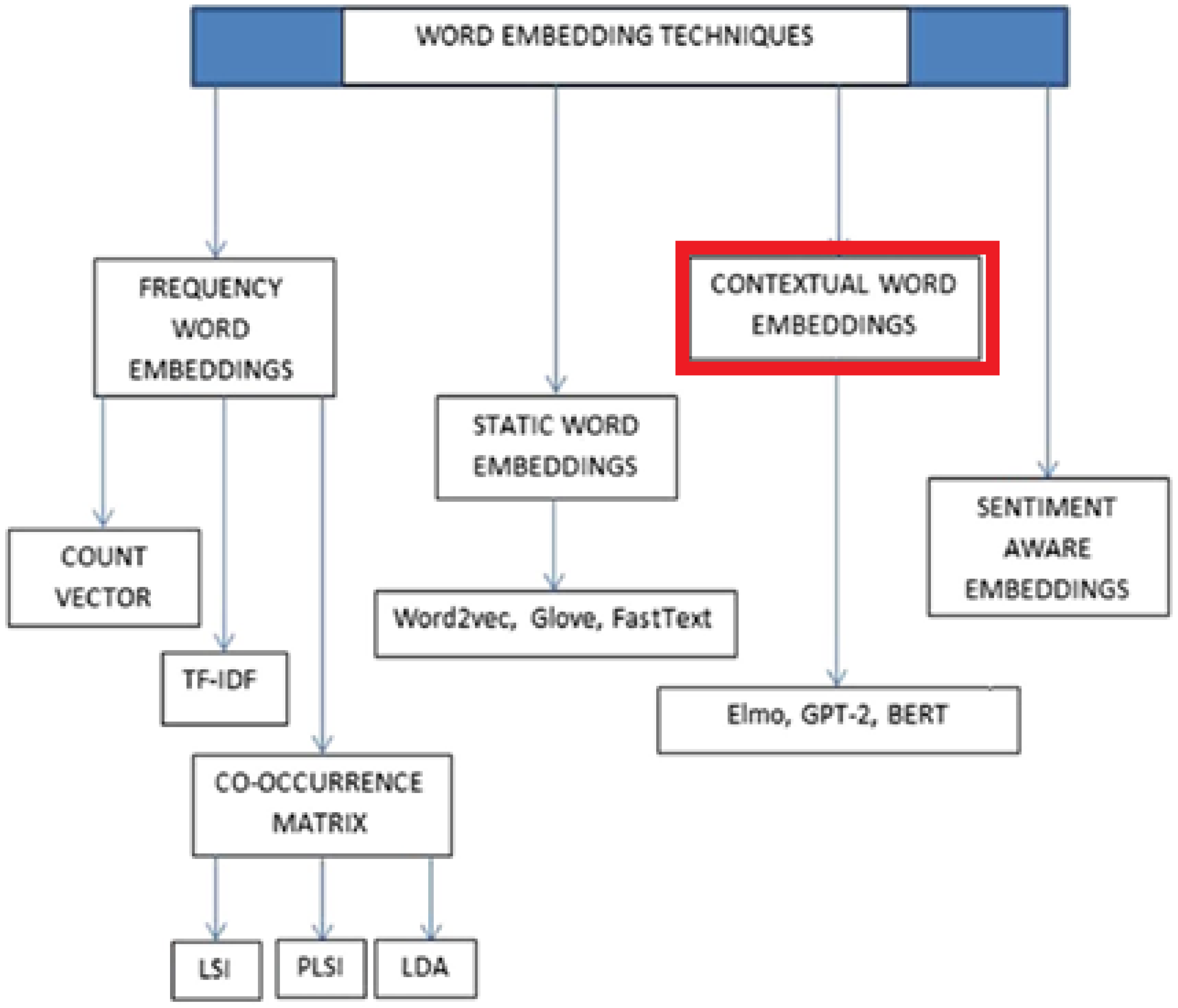
Figure 2.
Contextual embeddings of the word ‘draft’ where a scatter plot is shown in 2D via t-SNE (Van der Maaten and Hinton, 2008) on embedding vectors. Two main meaning classes are the verb and the noun.
Figure 2.
Contextual embeddings of the word ‘draft’ where a scatter plot is shown in 2D via t-SNE (Van der Maaten and Hinton, 2008) on embedding vectors. Two main meaning classes are the verb and the noun.
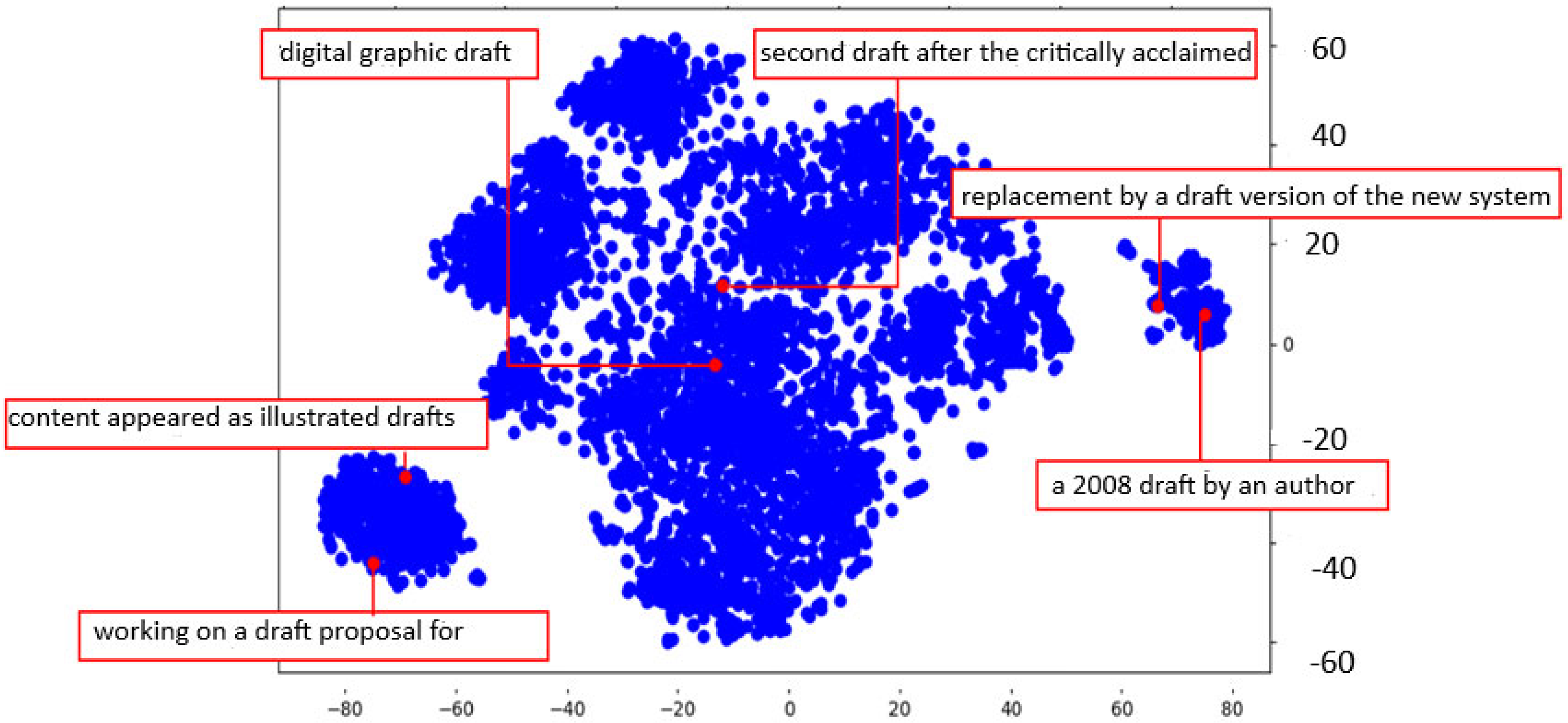
Figure 3.
Step-wise approximation of continuous embedding function.
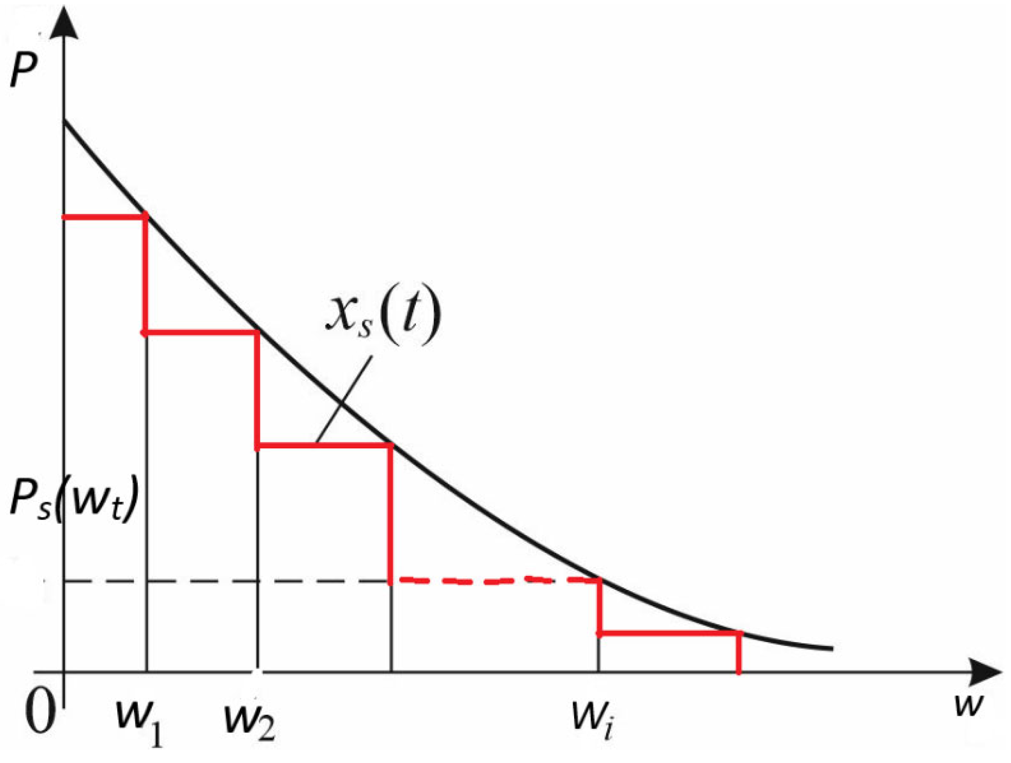
Figure 4.
Minimum entropy production and CBOW.
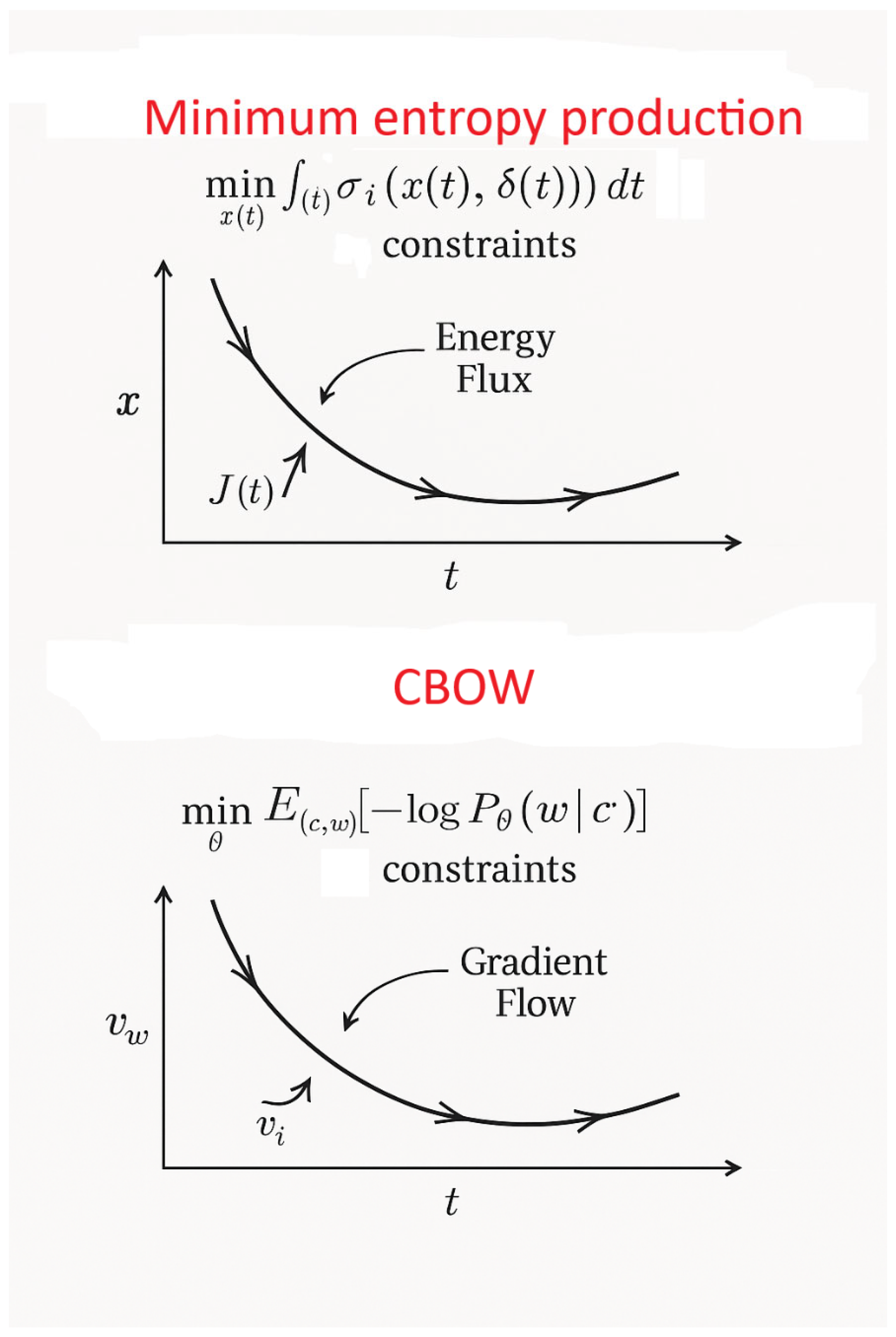
Figure 5.
Word2vec continuous profiles of words.
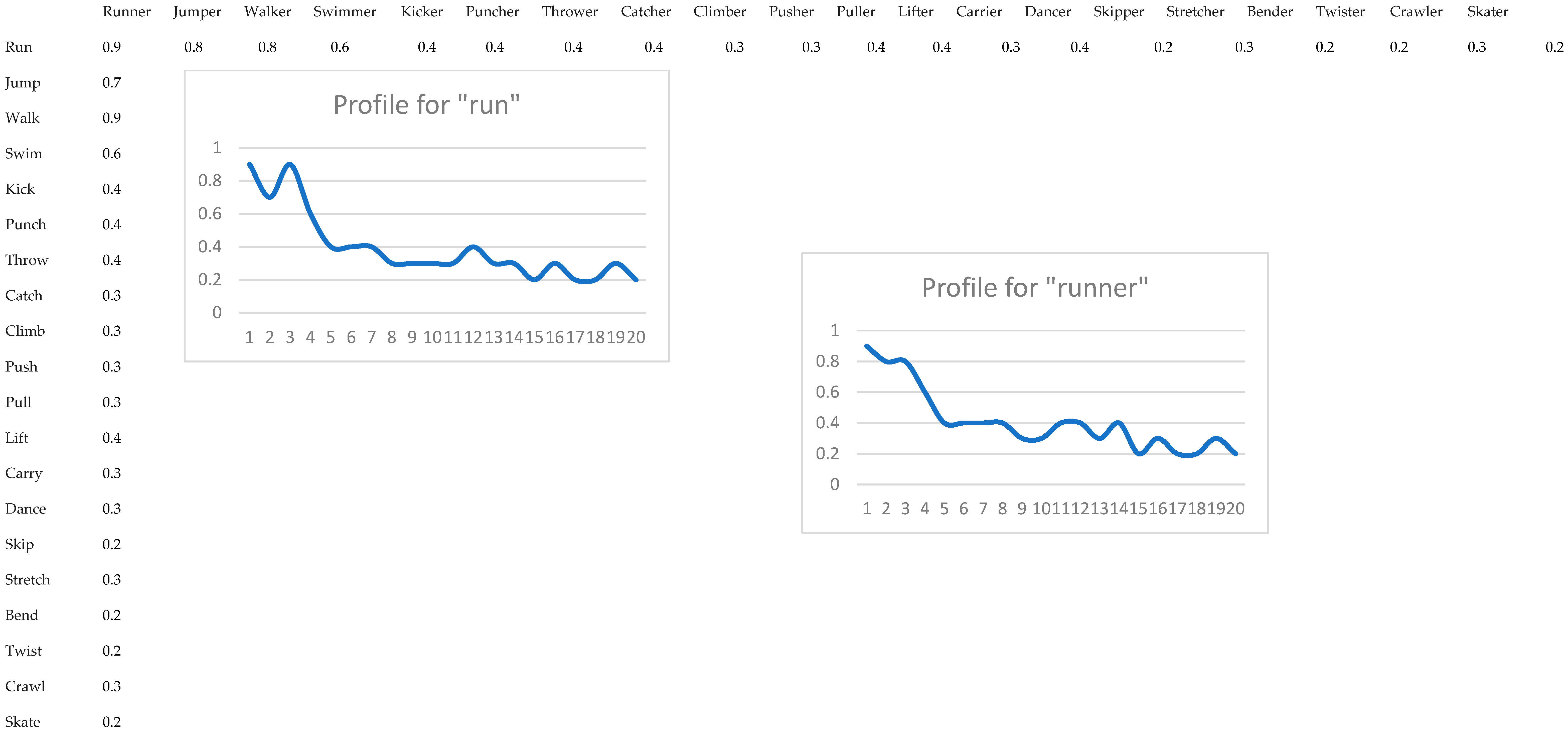
Figure 6.
Forming the evaluation dataset of tail entities where an improvement in embedding is needed.
Figure 6.
Forming the evaluation dataset of tail entities where an improvement in embedding is needed.
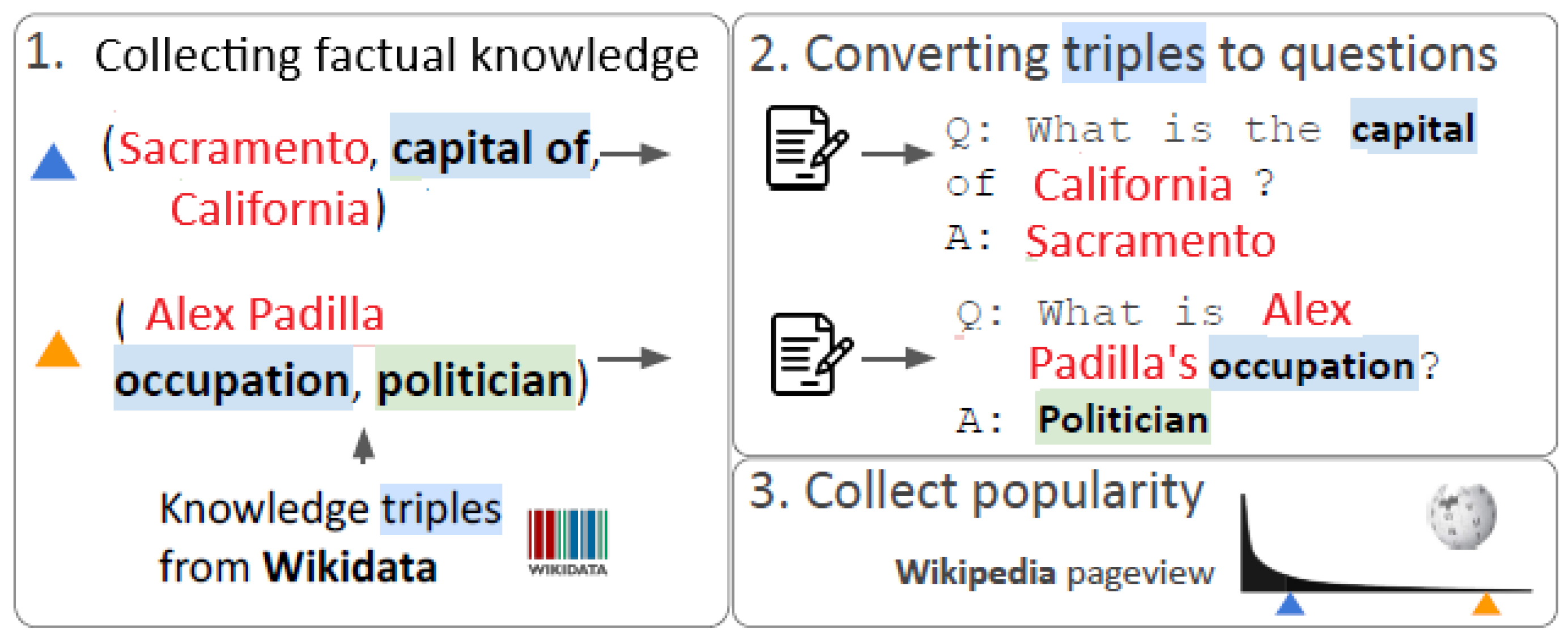

Table 1.
Thermodynamics and CBOW.
| Thermodynamic Concept | CBOW Analogy |
|---|---|
| Intensive variables xi(t) (e.g., temperature) | Word embeddings vi(t)∈Rd |
| Flow of matter/energy Ji(t) | Gradient flow during training dvi/dt |
| Entropy production rate σ(t) | Cross-entropy loss , or KL divergence from data |
| Constraint on process duration | Fixed training time or number of epochs |
| Constraint on average flux | Bounded gradient norm, limited context window |
| Law of evolution dxi/dt=f(x) | Stochastic gradient descent or Adam updates: |
Table 2.
NDCG@5 for infrequent and frequent entities for default, approximated and dynamic embeddings .
Table 2.
NDCG@5 for infrequent and frequent entities for default, approximated and dynamic embeddings .
| Default embedding | Step-wise approximation of embedding | Step-wise approximation of dynamic embedding | ||||
|---|---|---|---|---|---|---|
| Entity class | Popularity <103 | Popularity >105 | Popularity <103 | Popularity >105 | Popularity <103 | Popularity >105 |
| occupation | 0.720 | 0.783 | 0.768 | 0.798 | 0.724 | 0.745 |
| author | 0.743 | 0.793 | 0.775 | 0.824 | 0.816 | 0.765 |
| director | 0.681 | 0.759 | 0.698 | 0.775 | 0.698 | 0.731 |
| country | 0.692 | 0.701 | 0.686 | 0.703 | 0.677 | 0.726 |
| capital of | 0.732 | 0.750 | 0.803 | 0.783 | 0.754 | 0.733 |
| capital | 0.782 | 0.783 | 0.852 | 0.814 | 0.787 | 0.782 |
| religion | 0.742 | 0.795 | 0.762 | 0.816 | 0.741 | 0.789 |
| sport | 0.702 | 0.751 | 0.725 | 0.788 | 0.764 | 0.780 |
| producer | 0.681 | 0.715 | 0.692 | 0.711 | 0.750 | 0.743 |
| mother | 0.703 | 0.737 | 0.761 | 0.741 | 0.718 | 0.781 |
| place of birth | 0.725 | 0.741 | 0.772 | 0.738 | 0.783 | 0.699 |
| composer | 0.704 | 0.753 | 0.705 | 0.787 | 0.777 | 0.771 |
| genre | 0.726 | 0.724 | 0.776 | 0.765 | 0.804 | 0.710 |
| father | 0.706 | 0.740 | 0.775 | 0.744 | 0.723 | 0.716 |
| color | 0.689 | 0.726 | 0.718 | 0.730 | 0.714 | 0.721 |
| Average | 0.715 | 0.750 | 0.751 | 0.768 | 0.724 | 0.745 |
| Boost to baseline, approx. % | 4 | 2 | 5 | -0.05 | ||
Disclaimer/Publisher’s Note: The statements, opinions and data contained in all publications are solely those of the individual author(s) and contributor(s) and not of MDPI and/or the editor(s). MDPI and/or the editor(s) disclaim responsibility for any injury to people or property resulting from any ideas, methods, instructions or products referred to in the content. |
© 2025 by the authors. Licensee MDPI, Basel, Switzerland. This article is an open access article distributed under the terms and conditions of the Creative Commons Attribution (CC BY) license (http://creativecommons.org/licenses/by/4.0/).
Copyright: This open access article is published under a Creative Commons CC BY 4.0 license, which permit the free download, distribution, and reuse, provided that the author and preprint are cited in any reuse.


