Submitted:
07 July 2025
Posted:
07 July 2025
You are already at the latest version
Abstract
Turbulent boundary layer flows play a critical role in aerodynamic drag and flow control strategies. This study investigates the effects of wall-normal blowing on mean velocity profiles, turbulence statistics, and spectral properties. The experiment employs Particle Image Velocimetry to capture instantaneous velocity fields and visualize coherent structures, Laser Doppler Anemometry for high-resolution 1D velocity measurements with minimal flow disturbance, and Hot-Wire Anemometry to obtain time-resolved turbulence statistics at fine spatial scales as the reference. These techniques provide complementary insights into the redistribution of turbulent energy, Reynolds stresses, and spectral modifications due to blowing. The findings contribute to developing sustainable aerodynamic solutions by improving turbulence management and energy-efficient flow control strategies.
Keywords:
turbulent boundary layer
; uniform blowing
; flow control
; drag reduction
; coherent structures
; aerodynamics
; particle image velocimetry
; hot-wire anemometry
; laser Doppler anemometry
1. Introduction
According to EuHIT [1], Turbulent boundary layers remain one of the great unresolved challenges of 21st-century physics and fluid mechanics, as frequently emphasized in the literature. Turbulence mechanism found within turbulent boundary layer (TBL) flows play a crucial role in aerodynamic drag, heat transfer, and flow control applications. Among many other aerodynamic drag, particularly, skin-friction drag also known as friction drag, remains a critical challenge for aerodynamic efficiency in terrestrial and aerial vehicles. In subsonic transport aircraft, TBL-induced friction accounts for approximately 50% of total aerodynamic drag and significantly impacts fuel usage, operating costs, and environmental sustainability [2]. In response to international goals—such as the ICAO’s commitment to a 2% annual improvement in fuel efficiency—numerous flow control techniques have been proposed and investigated over the past decades. In a zero-pressure-gradient turbulent boundary layer (ZPGTBL), the flow develops naturally without external pressure gradients, making it a fundamental case for studying turbulence structures and subsequent friction drag outcomes.
In 2018 alone, the global airline industry was estimated to have spent 156€ billion on fuel. Given the substantial fuel expenditure in aviation [3], even marginal savings can significantly influence the success or failure of drag reduction strategies [4]. While aerodynamic shaping can mitigate form drag, surface friction—governed by near-wall turbulence, remains as the dominant controllable factor. Reducing this friction has the potential to substantially lower fuel consumption and carbon emissions. However, despite decades of study, the turbulence mechanisms remain partially understood. Moreover, Flow Control Technologies (FCTs) which refer to the techniques developed to reduce this so-called friction-drag in high-speed transportation, have novel characteristics of interaction with the turbulence mechanism. Although classical turbulent boundary layer flow is well investigated, it still lacks a proper description of the model under the influence of FCTs.
FCTs are broadly classified into passive and active methods, depending on the requirement of external energy. Passive methods like riblets, super-hydrophobic-surfaces (SHS), and Large-Eddy-Break-up Devices (LEBU) rely on geometric or material properties, whereas Active Flow Control Technologies such as Laminar Flow Control (LFC), Uniform Blowing (UB), Opposition Control, streamwise vortex actuators, and gas micro-bubbles utilize external energy sources to influence flow characteristics [4,5]. In order to distinguish between the surface boundary condition, classical TBL over smooth surface will be denoted as Standard Boundary Layer (SBL) hereafter.
Among these, UB has emerged as a highly promising method for turbulent drag reduction (TDR) in wall-bounded shear flows. Uniform blowing involves injecting fluid through a porous wall at a constant rate, [7] named it as Micro-Blowing Technique (MBT) considering the small perforations which is typically selected based on the Boundary Layer Thickness (BLT, ). Within TBL flows, velocity statistics are strongly influenced [8], downstream BLT is thickened (see Figure 1), coherence is improved [9], both convection and production are enhanced [10] and most importantly, outer layer turbulence processes are significantly influenced [11], which is the part of a TBL that contributes most of the cumulative production. In other words, outer layer turbulence costs more in terms of friction drag.
Hasanuzzaman et al. (2016) [8] investigated TBL flow control using UB with the help of Laser Doppler Anemometry (LDA) measurements over the range , where is the Reynolds number based on the momentum thickness . Typically, the viscous length scale , along with and the boundary layer thickness ( or ) 1, are used as the inner and outer scaling parameters, respectively. Here, denotes the friction velocity, the kinematic viscosity, and the free-stream velocity. However, these scaling parameters become insufficient when comparing velocity statistics between the SBL and UB cases, particularly at different blowing ratios (BR, mathmatically, F), where BR is defined as the ratio between the wall-normal velocity component due to blowing and , expressed as a percentage.
The experiment evaluated the effect of UB on velocity statistics and reported a 13% reduction in skin-friction drag at using a modest amount of blowing ( of ). Additionally, the study showed that UB increases the momentum thickness , which represents momentum loss in the boundary layer. A linear relationship between the increase in and the blowing intensity was established using a least-squares linear regression fit to empirical velocity profile data. They concluded that blowing enhances mixing and momentum transfer, and as a consequence, TBL grows faster.
An increase in momentum thickness () generally indicates greater momentum loss due to viscous effects and turbulence, that would have the same momentum loss per unit width as the actual boundary layer profile. A larger momentum thickness implies a greater momentum deficit and energy dissipation, and hence more momentum has been lost to the wall due to viscous shear stresses. In addition, the paper addressed another issue; the mean profiles of streamwise velocity under the influence of wall-normal blowing require different scaling than logarithmic or power-law. Although UB causes the boundary layer to grow, the introduced low-momentum fluid redistributes the velocity profile. As a result, the momentum deficit is reduced, especially near the wall. While momentum thickness may increase, the wall shear stress decreases, a favorable trade-off for drag reduction.
In order to understand the scaling in TBL flows, a vivid understanding of different layers of a TBL can be found from the logarithmic expression of the horizontal velocity profile as presented in Figure-Figure 2 from [5].
The mixing length hypothesis provides a theoretical framework to understand the mechanisms of transport within the TBL velocity profile. According to this hypothesis, the boundary layer can be divided into several distinct regions, as depicted in Figure 2, following the classification proposed by [6]. Closest to the wall lies the viscous sub-layer or VSL, defined for , where viscous (molecular) transport is dominant and the velocity profile is approximately linear. The streamwise velocity in this region can be modeled using Equation 1 which is depicted as a black line in Figure-Figure 2. Equation-1 holds valid for the VSL, e.g., the region near the wall, where viscosity begins to dominate the shear stress, and the velocity is proportional to wall distance.
Above this lies the buffer layer (BL), spanning the range , where both molecular and turbulent transport mechanisms are of comparable magnitude and in. The velocity distribution here is often described using Equation 4, following the model proposed by [13]. Further from the wall, in the region , lies the well-known logarithmic layer (LL), where turbulent transport becomes dominant and the mean velocity profile follows the classical logarithmic law expressed by Equation 2. This layer is characterized by self-similarity and Reynolds-number independence in the inertial sub-range. Beyond this, for , the flow enters the wake region (wake), where deviations from the logarithmic law are captured by the so-called law of the wake (Equation 3). It is important to note that the velocity profiles in all of these regions depend on the friction velocity , making the accurate determination of wall shear stress essential for any meaningful velocity scaling in turbulent boundary layers. In order to explain the drag reduction mechanism and to find the efficient flow control solution, a proper understanding of the turbulence process of the coherent structures is equally important as the statistical description.
Turbulence mechanisms, particularly the dynamics of coherent structures, play a crucial role in determining friction drag. These coherent structures consist primarily of organized vortical formations and often appear as packets of large, spatially distributed flow features. The classic description of these turbulent structures from [14] postulated that VSL and the outer region (combination of the LL and wake) is mostly populated with the so-called quasi-streamwise vortices and horse-shoe vortex respectively. It is the dissipation and transport process that determines the development of quasi-streamwise vortices transitioning into horseshoe vortices in the outer region.
Adrean et al. (2007) [15] classified these coherent structures based on their length scales , which can extend over long distances in the boundary layer, amplifying turbulent fluctuations and affecting mean flow properties. Based on their characteristic spatial scales, they are commonly classified as large-scale motions (LSMs) and very-large-scale motions (VLSMs). According to [16], LSMs have characteristics streamwise length of , whereas VLSMs can be as long as . These coherent structures dominate the outer region and interact with smaller-scale turbulence near the wall. However, these superstructures are the features that are only observed at sufficiently high Reynolds numbers and hence, incompressible aviation is also operated at high Reynolds numbers.
Experiments at high Reynolds numbers are essential for the development of effective flow control technologies aimed at large subsonic jet aircraft, which typically operate at chord Reynolds numbers up to and beyond [17]. While many laboratory experiments are conducted at significantly lower Reynolds numbers, such conditions may fail to represent the complex flow physics relevant to real operating environments. In particular, high Reynolds number turbulent boundary layers exhibit pronounced scale separation and increased interaction between VLSMs and near-wall small-scale structures, which play a critical role in friction drag generation [18]. As the Reynolds number increases beyond a certain threshold (e.g., ), the influence of outer-layer motions on turbulence production becomes comparable to or exceeds that of the inner layer [19]. These outer-layer dynamics is essential to capture when evaluating the performance of flow control strategies at sufficiently high Reynolds number. However, traditional intrusive techniques such as hot-wire anemometry (HWA) face limitations at high Reynolds numbers due to probe interference, particularly near the wall.
UB has been shown to weaken quasi-streamwise vortices in the near-wall region, which are responsible for much of the turbulent skin friction. This control mechanism promotes larger outer-layer structures and shifts turbulence production away from the wall, reducing the overall friction drag. [10] has shown that UB can reduce skin friction drag by disrupting the turbulence production cycle, especially in the logarithmic region of the boundary layer where large-scale motions dominate. This technique is particularly effective in reducing turbulent kinetic energy (TKE) production and weakening the self-sustaining turbulence mechanism. The same work also demonstrated that uniform blowing in a TBL flow led to a measurable decrease in wall-shear stress under zero pressure gradient conditions. The experiment was conducted at high Reynolds number where . They concluded that UB causes a thickening of the turbulent boundary layer due to increased wall-normal momentum transport. It modifies turbulence statistics by increasing the Reynolds shear stress, particularly in the outer region, and enhances turbulence intensities, especially in the streamwise direction. These effects are attributed to the altered near-wall dynamics and enhanced large-scale structures, as observed in high Reynolds number experiments using Stereo PIV measurements. In addition, the paper also developed a order empirical relationship for the Root-Mean-Square of the streamwise fluctuations under ’Stochastic forcing’ using UB. Figure 3 exhibits a quantitative influence on the coherent structures due to UB.
Recent experimental studies, such as those by [5], have used UB to manipulate turbulence structures. The introduction of uniform blowing at moderate Reynolds numbers enhances outer peaks in the boundary layer, leading to increased turbulent energy redistribution. This study demonstrated that controlled flow perturbations can alter turbulence statistics and potentially reduce skin friction drag.
’Stochastic forcing’ refers to the random and fluctuating nature of turbulence generation and its response to external flow control mechanisms. When uniform blowing is applied at the wall, it modifies the near-wall turbulence structures, leading to changes in mean velocity profiles, Reynolds stresses, and higher-order statistical moments. The injected momentum alters the balance between production and dissipation of turbulent kinetic energy, influencing coherent structures such as streaks and vortices. While uniform blowing itself is a deterministic control mechanism, its interaction with turbulence introduces stochastic effects, which can be quantified through statistical analysis of velocity fluctuations. By employing PIV, LDA, and HWA, we assess these effects across different spatial and temporal scales. Higher-order statistical moments provide insight into intermittency and turbulence modulation, offering a comprehensive view of how micro-blowing influences the stochastic nature of turbulence in a zero-pressure-gradient boundary layer.
The influence of wall-normal blowing on a TBL has been widely investigated due to its potential in drag reduction and flow control. However, the underlying physical mechanisms governing changes in mean flow characteristics, turbulence statistics, and coherent structures due to blowing remain an open question. This study aims to explore how wall-normal blowing affects the mean velocity profile and boundary layer thickness evolution in the downstream direction, as well as the modifications in turbulence statistics, particularly in the Reynolds stress components and root-mean-square velocity fluctuations, with an increasing F. Additionally, the research seeks to understand the changes in energy distribution within the turbulent boundary layer and their implications for coherent structures. A key question is whether blowing fundamentally alters the turbulence characteristics of the outer layer and how this, in turn, influences near-wall turbulence dynamics. Furthermore, determining the optimal blowing parameters that maximize drag reduction while maintaining flow stability remains a critical challenge. The spectral properties of turbulence, including power spectra and cross-spectra, must also be analyzed to assess their evolution with varying blowing intensities. Finally, the geometric configuration of the perforated surface is expected to play a crucial role in the efficiency of flow control, and its impact warrants detailed investigation. Through experimental measurements and scaling analyses, this study aims to establish an empirical and theoretical framework to better understand the influence of wall-normal blowing on TBL, ultimately contributing to the development of efficient aerodynamic flow control strategies.
In a subsequent study under the [11] reported experiments in a ZPGTBL, where a wide variation of moderate Reynolds number flow was investigated at different BRs of UB. The maximum TDR of 30% was achieved using UB through perforated plates. The technique offers advantages such as simplicity, scalability, and substantial energy savings, making it a valuable candidate for future TDR solutions, especially in meeting stringent CO2 reduction targets set by organizations like ICAO and Airbus.
Applying PIV in a high-speed complex flow is a challenging task. The state-of-the-art PIV system used in the aerodynamic community is expensive and yet, often lacks capacity to provide measurement data with sufficient accuracy. Despite its widespread use in experimental fluid mechanics, PIV exhibits several limitations when applied to TBL flows. Firstly, near-wall measurements using classical PIV are often unreliable due to laser reflections and limited resolution within the viscous sub-layer, which significantly affects the accuracy of wall-shear stress estimation. High-magnification PIV can enhance near-wall resolution but requires high seeding density and is sensitive to boundary condition changes caused by flow control experiments. Secondly, PIV struggles to resolve the full range of turbulent scales simultaneously, especially in thick boundary layers where large field of view (FOV) and multiple overlapping cameras are necessary, increasing the complexity and cost of the setup. Additionally, convergence issues arise for secondary velocity components (wall-normal and spanwise) and Reynolds shear stress, even with large sample sizes. Time-resolved PIV (TRPIV) introduces further challenges due to memory limitations of high-speed cameras and the trade-off between spatial resolution and acquisition rate. Moreover, insufficient seeding in the near-wall region, particularly under uniform blowing or flow control conditions, exacerbates measurement difficulties. These issues collectively limit the spatial and temporal resolution of PIV, making it difficult to capture accurate, high-fidelity velocity fields throughout the entire TBL. For details, interested readers are referred to [12].
This motivates the present research, which investigates uniform blowing as an active flow control strategy to mitigate skin-friction drag by altering the turbulence structure within the boundary layer. This publication reports on a wind tunnel experiment with a unique approach by applying PIV to a very small FOV at high speed incompressible, aerodynamic flow, the PIV measurement presented here corresponds to the . Non-intrusive measurement methods such as PIV provide a more reliable means to study outer-layer dynamics and handle large volumes of data efficiently. The present high Reynolds number experiments employ PIV to investigate the role of large-scale motions in turbulence production and assess the statistical impact of flow control measures. These insights are critical for designing models and technologies capable of reducing skin-friction drag in aero-engineering applications operating within the high Reynolds number regime. Subsequently, PIV measurements were complemented with reference LDA and HWA data.
2. Methodology
2.1. Experimental setup
The experiment was conducted using a closed-return, Göttingen-type subsonic wind tunnel at Brandenburg University of Technology, Germany. The tunnel is designed for reliable performance up to a free-stream velocity of m/s, corresponding to a Reynolds number based on the characteristic length of the flat plate, . The flow in the test section is highly uniform, with turbulence intensity slightly above 0.5%. The contraction ratio is 1:5.5, and thermal stability is maintained within ±0.1 K using a heat exchanger installed upstream of the honeycomb grids. The measurement section dimensions are m3 (width × height × length), with optical access through low-distortion glass walls for non-intrusive flow measurements.
Flow seeding was achieved using an aerosol generator (AMT 230, Topas Co.) with Di-Ethyl-Hexyl-Sebacat (DEHS) particles, having a median diameter of approximately m. These particles maintain a viable presence in the flow for up to four hours. A total of 32 TBL profiles were measured at a fixed streamwise location.
The flat plate used was fabricated from smooth, anodized aluminum to create a matte black surface and prevent laser reflections. It measured m3 (length × width × thickness) and was mounted horizontally inside the test section (see Figure 4, reproduced from [11]). The bottom-left corner of Figure 4(a) is used as the origin in a Cartesian coordinate system: the streamwise, wall-normal, and spanwise directions align with the x-, y-, and z-axes, respectively. Measurements were performed at approximately 58% streamwise and 33% spanwise positions on the plate.
An elliptical leading edge was designed based on Smits et al. [20], and the boundary layer was tripped using a DYMO tape label (’x’ symbol, mm2, ) placed 50 mm downstream from the leading edge (see Figure 4). The flat plate included four interchangeable segments to enable varying the blowing region. For this study, two solid sections ( mm3) were installed upstream and downstream of the perforated section, which occupied the third slot. This configuration positioned the perforated surface between approximately 52% and 70% of the plate length.
Reference SBL measurements were obtained using the solid plate for in the range using LDA. Subsequently, the upstream region was replaced with a Modular Blowing assembly to introduce wall-normal blowing.
The UB wall was constructed from a 1 mm thick perforated anodized aluminum plate with external dimensions of mm2 (width × length). Electron beam drilling ensured high precision in hole diameter and placement. Figure 4(c) shows a microscopic view of the perforated region. Each hole had a diameter mm (approximately 20 viscous length scale e.g at , see Figure 4(d)) and spacing of 0.4 mm, giving a hole-to-pitch ratio . The surface roughness before perforation was mm. Post-fabrication measurements confirmed no significant change in roughness, leading to , which satisfies the smooth-wall assumption [21].
The perforated plate porosity was , and the hole aspect ratio was , enabling laminar flow through each hole at low hole Reynolds numbers 2. The internal blowing chamber measured m2, resulting in an effective exit area . The chamber was hermetically sealed with layered screen meshes to ensure uniform pressure distribution across the MBT wall.
Blowing was implemented as an open-loop control scheme. Ambient-temperature air was supplied via a compressor through a digital flow meter (DFM-47, Aalborg), accurate to . The volumetric flow rate was used to compute the wall-normal blowing velocity as . This analytical value was validated using LDA measurements at mm from the wall. Therefore, friction coefficient, is measured from near wall LDA data from Hasanuzzaman et al. (2022) [11] as reference measurements to the PIV data.
2.2. Measurement system
The PIV system from Dantec Dynamics comprised the following hardware components: FlowSense 2M camera, double-pulse Litron laser, timer box, synchronizer, and acquisition PC.
For high-speed aerodynamic measurements, strong illumination is typically required to capture accurate flow structures. Although the boundary layer flow in the present study had a relatively low free-stream velocity (less than Mach 0.2), the resulting BLT was small ( mm), owing to the limited development length of the flat plate.
Figure 5(a) shows a photograph of the PIV hardware and optical components installed in the BTU wind tunnel test section. A Dantec DualPower 200-15 Nd:YAG laser system (Litron, Nova Instruments) was used to provide illumination. This system consists of a dual-cavity, flash-lamp-pumped, double-pulse laser, optimized for PIV applications. It is equipped with a Q-switch to enable precise synchronization with the camera system. At an acquisition frequency of 15 Hz, the system delivered two pulses of 200 mJ per cavity at a wavelength of .
Image acquisition was performed using a FlowSense 2M camera with a objective lens. The camera features a 2-megapixel CCD sensor, capable of capturing images at 8- or 10-bit resolution. In this experiment, 10-bit resolution was used to enhance measurement fidelity. For each test configuration, 240 double-pulse image pairs were recorded at a frame rate of 15 Hz, corresponding to an acquisition time of approximately 16 seconds.
The free-stream velocity in the wind tunnel varied between 5 and 35 m/s. To optimize particle image displacement, the inter-frame time delay was adjusted between 50 and 5 s. This setting ensured that average particle displacements remained within the 7–12 pixel range, which is optimal for PIV processing, especially in wall-bounded turbulent flows where strong velocity gradients are present.
Prior to data collection, a calibration procedure was performed using a checkerboard target to convert pixel displacements into physical distances. Figure 5(b) illustrates the optical path and alignment used for the FOV setup. The CCD camera captured a two-dimensional FOV measuring m2 in the wall-normal and streamwise directions, as shown in Figure 5(c). This resulted in a spatial resolution of 60.2 pixels/mm in the wall-normal direction and 56.2 pixels/mm in the streamwise direction, providing approximately 5 velocity vectors per millimeter in each dimension.
2.3. Image Processing
Following acquisition, the raw double-pulse dark images (DI) were processed using Dantec Dynamics’ proprietary software suite. The initial step involved assigning each DI sequence to the Image Processing Library (IPL), where a median low-pass filter (MF) was applied. This non-linear filter replaces the central pixel within each kernel window with the median grayscale intensity of the surrounding pixels, effectively suppressing high-frequency noise while preserving edge information—crucial for resolving boundary layers where the wall-normal location of the interface is not known a priori.
Each set of 240 DI pairs was then used to compute a mean background image via an image arithmetic routine. Specifically, the average grayscale intensity for each pixel location was determined over time, and this mean background—estimated using morphological opening—was subtracted from each frame to enhance particle visibility and minimize background light reflections.
Once image conditioning was complete, velocity vector estimation was performed using the adaptive correlation method available in the Analysis Sequence Library. No a priori windowing or additional filters were applied. The algorithm begins with a relatively large initial interrogation area (IA), typically a multiple of the final IA size, and refines the displacement estimates iteratively. In this study, an initial IA of pixels was used, followed by a single refinement step to a final IA of pixels. A 50% overlap was employed in both the horizontal and vertical directions to maintain high spatial resolution.
Velocity vectors were calculated by determining the mean particle displacement within each IA. To ensure data quality and eliminate spurious vectors, a robust validation scheme was employed. Displacement vectors were computed using a central difference scheme, which improves the accuracy of velocity gradient estimation.
Peak detection in the cross-correlation analysis adhered to a strict threshold criterion: the primary correlation peak had to exceed the second-highest peak by a factor of at least 1.2 for the displacement to be considered valid. No local neighborhood validation or smoothing was applied.
Displacement fields, initially in pixel units, were mapped to physical space using calibration images captured prior to measurement. A third-order polynomial transformation was used to convert image coordinates to physical coordinates. This process yielded a final spatial resolution of approximately 5 vectors/mm in both the wall-normal and streamwise directions.
Statistical moments of the velocity signal were computed using transit-time weighting, as defined in Equation 6, where N denotes the total number of samples and is the transit time of the seeding particle traversing the LDA measurement volume.
The first four statistical moments—mean, root-mean-square (RMS), skewness, and flatness—of the streamwise velocity component (u) were calculated using Equations 7, 8, 9, and 10, respectively. An identical approach was applied to compute the corresponding statistical moments for the wall-normal velocity component (v).
Inner or viscous length scaling in TBLs using wall variables such as friction velocity () and kinematic viscosity () is commonly done via Clauser fitting to the logarithmic law [22,23]). However, at low Reynolds numbers, the limited extent of the logarithmic region makes fitting unreliable. Moreover, at moderate Reynolds numbers with wall-normal blowing, the friction velocity is altered, rendering inner scaling-based fitting ineffective. Alternative techniques like oil film interferometry (OFI), HWA, or Preston tubes may also suffer from inaccuracies, especially near the wall [24].
In this study, a direct method based on LDA measurements in the viscous sublayer was used. Assuming a two-dimensional boundary layer near the wall, the slope of the mean velocity profile was identified using a sliding regression technique. A threshold correlation coefficient () was applied to detect the linear region of the velocity profile along uncorrected wall distances. The beginning of the stable linear plateau determined the first valid measurement point.
Once identified, the number of consecutive points within this threshold was used to fit the relationship , which allowed correction of the wall distance (). The corrected velocity gradient was then used to calculate the wall shear stress (), and subsequently, the friction velocity () and friction coefficient () for all datasets.
Wall distance corrections were constrained to . It was also observed that the number of valid near-wall points decreased with increasing Reynolds number due to the thinning of the viscous sub-layer. Interested readers are referred to [5] for the detailed procedure of the near-wall velocity measurements.
The uncertainty in velocity measurements derived from PIV was estimated based on factors including particle image density, correlation peak sharpness, and interrogation window size. For the acquisition parameters used in this study, the overall uncertainty was found to be within of the freestream velocity. This level of accuracy aligns with standard benchmarks for near-wall PIV measurements in turbulent boundary layer flows.
3. Results
3.1. Statistical assessment
Figure 6(a) and (b) present the mean velocity profiles under SBL conditions using three different measurement techniques: PIV, LDA, and HWA. These methods correspond to wall-normal sampling densities of approximately , , and points per meter, respectively. The averaging was done using Equation-6 and . In Figure 6(a), the velocity profiles are plotted using outer scaling parameters. PIV measurements are compared with reference LDA and HWA data from [11] and [23] respectively. The reference HWA profile corresponds to a turbulent boundary layer at , which is slightly higher than that of the current LDA and PIV datasets, leading to small deviations in the outer region.
The inset in Figure 6(a) highlights the near-wall region, illustrating the relative proximity of the first valid measurement points from each technique. LDA captures data closest to the wall, followed by HWA, whose first valid point is approximately 2.5 times further from the wall than that of LDA. The PIV technique captures its first point at approximately twice the distance of HWA’s, indicating its relatively coarser resolution in the near-wall region.
Figure 6(b) displays the same velocity profiles plotted using inner (viscous) scaling, i.e., normalized by the wall-shear velocity () and viscous length scale (). The LDA and HWA datasets are scaled using their respective wall-shear stress measurements, while the PIV profile is scaled using the wall-shear stress estimated from LDA data at the same Reynolds number. Due to wall reflections, the first two data points obtained from the PIV measurements exhibit deviations in the overlap region.
Each viscous wall unit corresponds approximately to one micrometer, i.e., m. In both outer and inner scaling representations, the data from all three measurement techniques show excellent agreement throughout the boundary layer. Additionally, empirical relationships such as linear (Equation-1) and logarithmic (Equation-2) profile representations are included in both figures for comparison.
Higher-order moments of turbulent velocity fluctuations are presented in Figure 7(a) and (b), plotted using outer and inner (viscous) scaling, respectively. The RMS of the velocity fluctuations was calculated using Equation for both the streamwise () and wall-normal () components. It is observed that exhibits better accuracy and consistency compared to . In particular, the agreement among all three measurement techniques is good within the outer region of the boundary layer.
Furthermore, third- and fourth-order moments—skewness and flatness—of the streamwise velocity fluctuations are shown in Figure 8(a) and (b), both plotted using viscous length scaling. Skewness () and flatness () were computed using Equations and , respectively. The skewness profiles generally show good agreement among the datasets, except in the near-wall region. However, flatness values from HWA deviate from those of LDA and PIV, likely due to the influence of higher Reynolds number effects in the HWA reference data.
Figure 10(a) and (c) show the instantaneous velocity vector fields for the SBL and UB cases at and , respectively. The original velocity field consists of vectors. For clarity, only every third vector in both the horizontal and vertical directions is plotted in Figure 10(a) and (c). Arrows represent the local velocity vectors, computed from the horizontal and vertical components of the fluctuating velocity field. The background color contours display the instantaneous streamwise velocity component u.
Figure 10(b) and (d) present the corresponding vorticity fields, computed as , for the same SBL and UB cases shown in (a) and (c), respectively. While instantaneous velocity fields may not fully capture the statistical behavior of turbulence, they qualitatively illustrate the physical dimensions and structures of the resolved turbulent scales.
Experimental methods such as LDA and PIV are widely used for investigating TBLs, but both face inherent limitations in resolving the near-wall region, particularly for . This zone is characterized by steep velocity gradients and small-scale turbulence, which demand high spatial and temporal resolution. Such conditions pose challenges due to optical access constraints and measurement fidelity. Nonetheless, the near-wall region remains critically important for flow control strategies, drag-reduction techniques, and the development of wall-resolved turbulence models.
To evaluate the accuracy of experimental techniques in capturing this region, Figure 9(a) and (b) compare the first- and second-order statistical moments of the streamwise velocity component. These measurements were obtained from PIV and LDA at and are compared against Direct Numerical Simulation (DNS) data at by Schlatter and Örlü [25]. The LDA dataset used is from Hasanuzzaman et al. [11] and serves as an experimental reference.
Figure 9(a) presents the mean velocity profiles ( versus ). The agreement between PIV, LDA, and DNS is excellent across the buffer and logarithmic regions. Notable deviations occur within the viscous sub-layer (), where PIV fails to capture the sharp near-wall gradient. This is likely due to wall reflections and insufficient wall-normal resolution. LDA performs better in this region but still under-predicts velocity relative to DNS in the first few wall units, as it cannot fully resolve the smallest scales.
Figure 9(b) shows the rms of streamwise velocity fluctuations, . The peak associated with buffer-layer turbulence is reasonably captured by LDA and DNS, while PIV underestimates this due to its lower spatial resolution. All three datasets show excellent agreement at the second peak (around ), corresponding to large-scale turbulent structures.
These observations suggest that for high-speed TBL flows with limited boundary layer thickness, LDA is more suitable for capturing near-wall small-scale dynamics, whereas PIV is better for resolving outer-layer structures over a larger field of view. The selection of measurement technique ultimately depends on a trade-off between spatial resolution, optical access, post-processing effort, and the specific flow features of interest.
3.2. Uniform Blowing
Figure 10 presents a comparative analysis of the instantaneous velocity and vorticity fields for SBL and UB conditions. While instantaneous velocity fields may not fully capture the statistical behavior of turbulence, they qualitatively illustrate the physical dimensions and structures of the resolved turbulent scales. The instantaneous velocity vector fields for the SBL and UB cases at and , respectively. The original velocity field consists of vectors. For clarity, only every third vector in both the horizontal and vertical directions is plotted in Figure 10(a) and (c).
Figure 10 (a) and (c) show the instantaneous velocity vectors overlaid on contours of streamwise velocity for the SBL and UB cases, respectively. In the SBL case (a), the near-wall region () exhibits low-speed streaks and inclined vectors that are characteristic of coherent structures in turbulent boundary layers. The velocity magnitude increases with wall-normal distance, transitioning into a more uniform and aligned streamwise flow. In contrast, the UB case in sub-figure (c) shows a visibly thickened boundary layer and a broader near-wall mixing region. The streamwise velocity contours are displaced upward, and the vector field reveals disrupted coherence, indicating that wall-normal momentum injection alters the turbulence structure and interferes with the regeneration cycle of near-wall streaks and vortices.
The corresponding vorticity fields in sub-figures (b) and (d) further highlight the effects of uniform blowing. The vorticity fields were computed as . In the SBL case (b), vorticity is concentrated near the wall, revealing compact and localized vortical structures that dominate the near-wall turbulence production. Conversely, the UB case (d) displays a more diffuse and vertically distributed vorticity field, signifying a weakening and redistribution of vortical structures due to the imposed blowing. This broader distribution is consistent with theoretical predictions of drag reduction mechanisms via uniform blowing, where the near-wall cycle is disrupted, and the peak turbulence production is pushed away from the wall.
Figure 10.
(a) Instantaneous vector plots of velocity components with contours of streamwise velocity at SBL condition, (b) Vorticity of the velocity vectors at SBL conditions, (c) Vector plots of velocity components with contours of streamwise velocity at UB, (d) orticity of the velocity vectors at UB conditions.
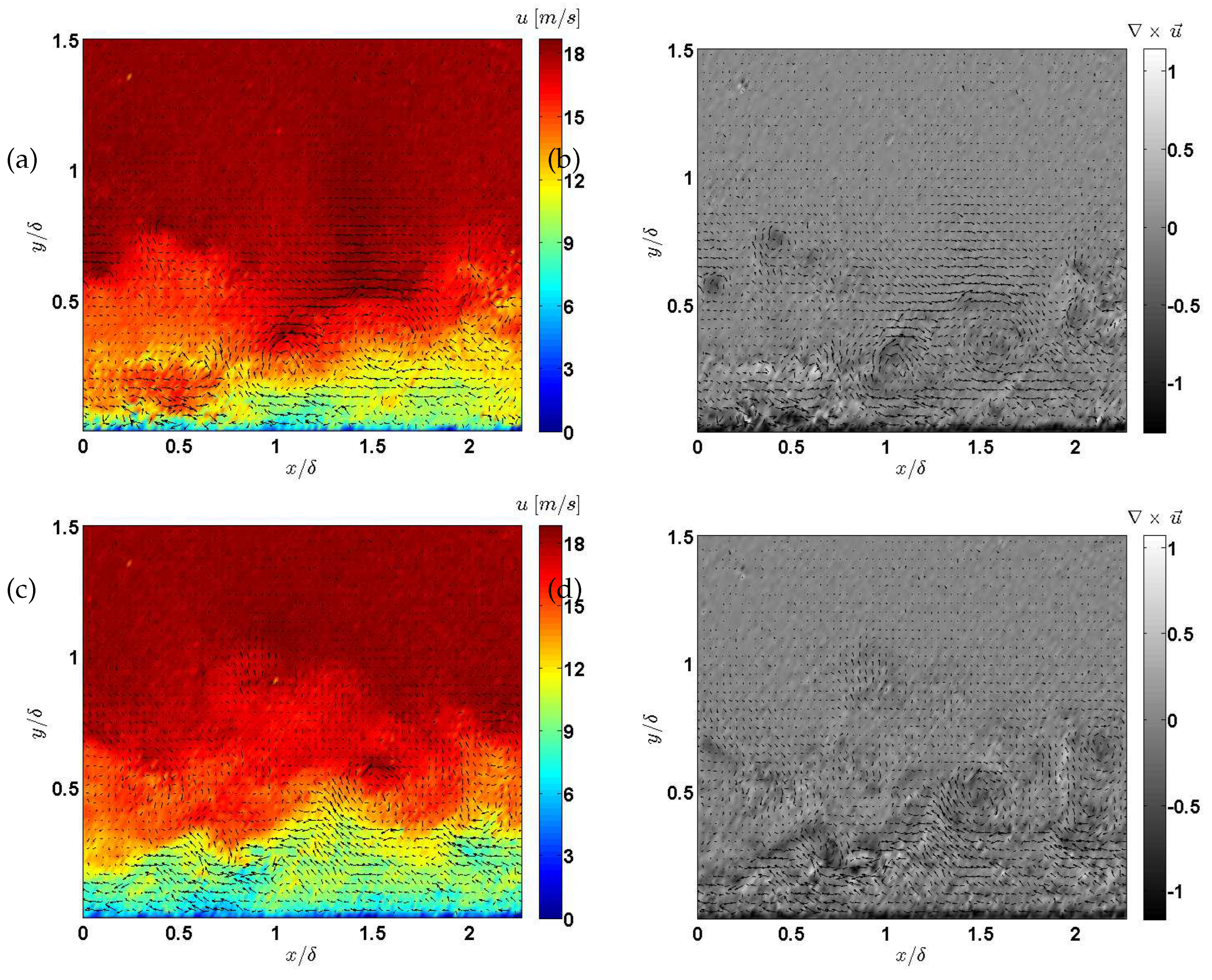
These qualitative observations align well with the statistical moment analysis conducted using transit-time-weighted LDA data. The altered velocity and vorticity structures observed in the UB case suggest modified profiles of root-mean-square fluctuations, reduced skewness, and lower flatness, particularly near the wall. Overall, the figures illustrate how uniform blowing modulates turbulence by thickening the boundary layer, reducing the coherence of near-wall structures, and redistributing vorticity—key mechanisms that contribute to friction drag reduction.
Shear flows are reflection of the wall condition. The quantitative friction co-efficient at SBL and different UB rates were measured from the direct measurements using reference LDA.
Figure 11.
(a) Friction co-efficient , (b) Shape factor () against reference . In both the figures gray dashed line indicate DNS data from [25].
Figure 11.
(a) Friction co-efficient , (b) Shape factor () against reference . In both the figures gray dashed line indicate DNS data from [25].
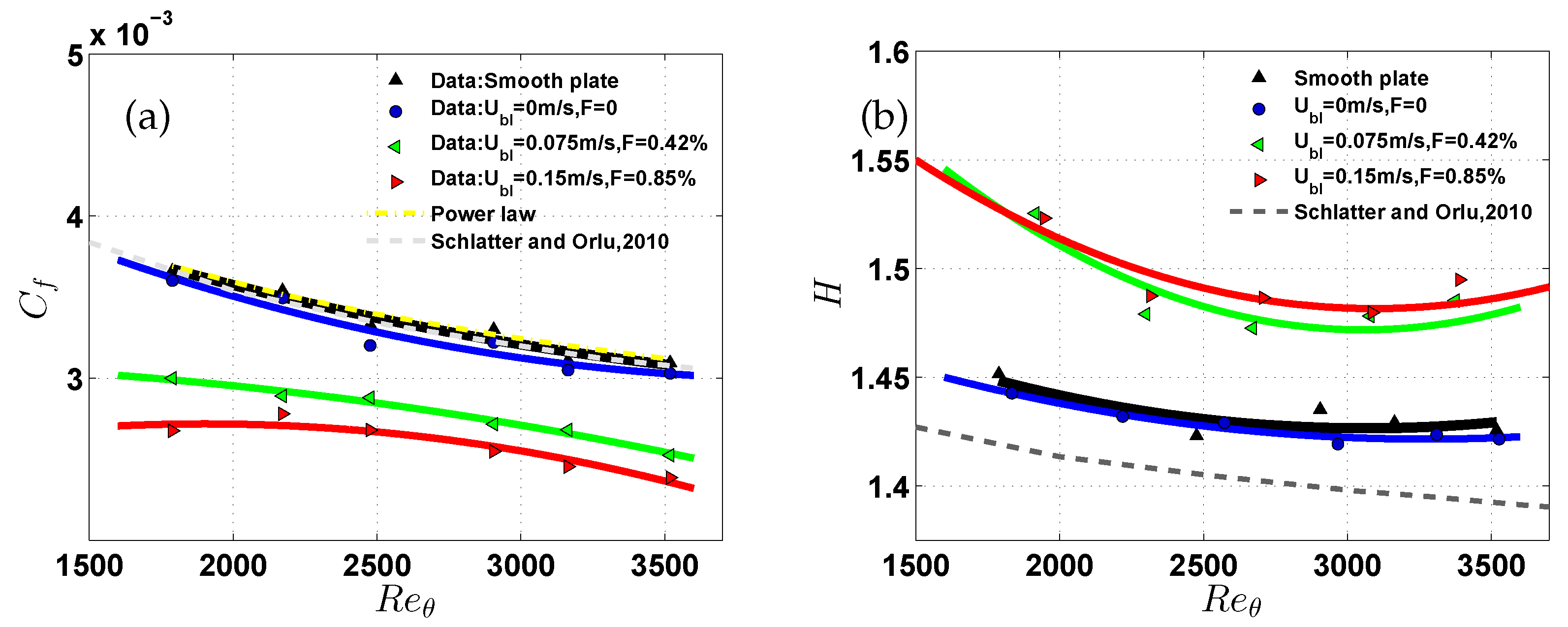
Figure 11(a) presents the streamwise evolution of the friction coefficient () plotted against the momentum-thickness Reynolds number () for different wall-normal blowing velocities. The baseline case, denoted by black triangles, represents SBL conditions and serves as the reference for comparison. Overlaid are experimental data corresponding to UB applied through a perforated wall at different fixed wall-normal velocities: m/s (no blowing, blue circles), m/s (green left-pointing triangles), and m/s (red right-pointing triangles), corresponding to blowing ratios of 0%, 0.42%, and 0.85%, respectively.
To isolate the effect of uniform blowing on skin-friction drag, values are plotted against the from the reference SBL configuration. This ensures that any reduction in due to blowing is not masked by the inherent increase in caused by boundary layer thickening. The reference smooth wall data is compared with two benchmarks: the power-law model proposed by Smits et al. (1983) [20] with a constant , and experimental data from Schlatter and Örlü (2013) [25], which slightly underpredict the trend, likely due to measurement limitations in the near-wall region.
The present SBL data (black triangles and blue circles) show good agreement with the Smits power-law trend [20]. The case with perforated wall but no blowing (blue circles) shows only a minor deviation, suggesting that surface perforation alone has a negligible impact on wall-shear stress. However, once uniform blowing is introduced (green and red curves), a clear reduction in is observed. At m/s, the curve shifts downward, and at m/s, the reduction becomes more pronounced, reaching values close to below the baseline.
Interestingly, although blowing thickens the boundary layer (increasing ), the reduction in does not grow proportionally. This is because the blowing velocity is fixed, while the boundary layer momentum increases with streamwise distance, effectively reducing the blowing ratio (F). This decline in F with increasing explains why the drag-reducing effect plateaus beyond , and then gradually decreases at higher .
Moreover, the measurement uncertainty increases at higher , primarily due to fewer valid data points within the viscous sublayer (as shown in Figure 8(c), not displayed here), where accurate slope detection for wall-shear estimation becomes more difficult. This limitation impacts the reliability of values above .
Although not explicitly shown in this figure, uniform blowing also induces significant changes to integral boundary layer properties such as boundary layer thickness (), displacement thickness ( or ), momentum thickness (), and shape factor (H), as documented in Hasanuzzaman (2021) [5].
Figure 11(b) shows the evolution of the boundary layer shape factor, defined as , with respect to for various UB conditions. In this figure, legend indication is the same as Figure 11(a) The shape factor is a critical indicator of boundary layer structure, reflecting the relative fullness of the velocity profile—higher values generally correspond to thicker boundary layers with stronger velocity deficits near the wall.
The SBL reference case shows a monotonic decrease in H with increasing , consistent with the expected development of a turbulent boundary layer. This trend is well aligned with the no-blowing perforated surface (blue circles), which exhibits negligible deviation, confirming that surface perforation alone does not alter the boundary layer structure significantly. Both these cases also align closely with the empirical data of [25], shown by the dashed-gray line.
In contrast, when uniform blowing is applied through the perforated wall—at BR, % and % a marked increase in the shape factor is observed across the full range of . This trend reflects the fact that wall-normal momentum injection opposes the normal boundary layer development, resulting in a fuller velocity profile with increased displacement thickness () relative to momentum thickness ().
Interestingly, the H values under blowing conditions show a non-monotonic trend: they decrease slightly with up to around 2500, then level off or slightly increase. This is attributed to the fixed blowing velocity (), which leads to a decreasing blowing ratio () as the free-stream velocity and boundary layer momentum increase with . As a result, the influence of blowing becomes less dominant at higher Reynolds numbers, leading to a plateauing of the shape factor.
Figure 12.
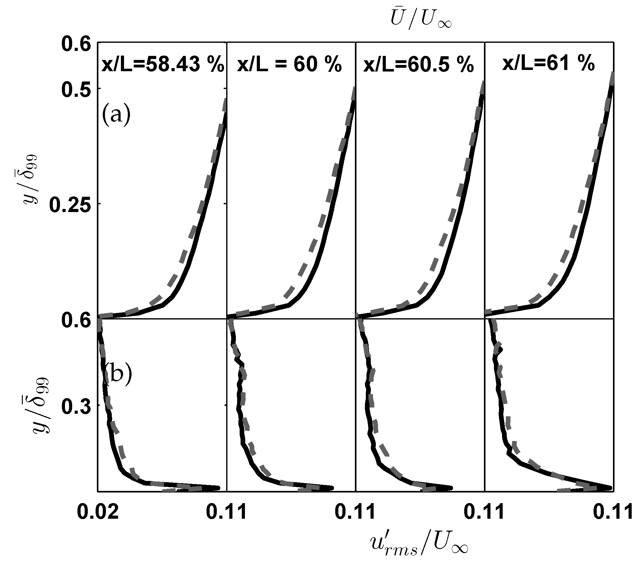
Spatial development of the TBL thickness () at different downstream stations, comparing SBL and UB, where, SBL is indicated with ’’ and UB at blowing ratio, F = 0.85% is indicated with ’– –’ (a) outer-scaled mean velocity profiles, (b) outer-scaled mean rms profiles of streamwise fluctuations.
Figure 12.
Spatial development of the TBL thickness () at different downstream stations, comparing SBL and UB, where, SBL is indicated with ’’ and UB at blowing ratio, F = 0.85% is indicated with ’– –’ (a) outer-scaled mean velocity profiles, (b) outer-scaled mean rms profiles of streamwise fluctuations.
Additionally, the observed shape factor values in the UB cases (–) remain higher than the SBL values (–), consistent with the presence of an external momentum source (e.g UB). These results support earlier findings by Hasanuzzaman (2021) [5], which reported that uniform blowing leads to substantial modification of integral boundary layer properties, not just local skin-friction reduction.
Figure 13 presents (a) outer-scaled mean streamwise velocity () and (b) streamwise turbulence intensity () profiles along wall distance at different downstream stations e.g . The canonical SBL profile is shown as solid black line, while the UB case at is represented by gray dashed line. Wall-normal distance is normalized by .
The analysis of velocity profiles reveals characteristic modifications induced by uniform blowing. As shown in Figure 13(a), the UB case exhibits three distinct influences, (1) boundary layer thickening, with discernible deviations from the canonical profile for , (2) Enhanced turbulence intensity () in the outer region () and (3) potential viscous sub-layer stabilization ().
UB at F=0.85% modifies the TBL structure without flow separation, aligning with the outcomes suggested by Hasanuzzaman et al (2020)[10] and Hasanuzzaman et al (2016)[8]. Quantify the displacement thickness change () to highlight control efficiency. These observations suggest increased vertical momentum transfer while maintaining attached flow conditions at this blowing ratio. The spatial consistency across multiple streamwise locations () confirms the stochastic equilibrium of the flow. This behavior aligns with previous studies of low-momentum injection, though quantitative assessment of would further clarify the control effectiveness.
Figure 13 quantifies the streamwise development of boundary layer thickness under upstream blowing conditions. Figure-Figure 13(a) plots the dimensional streamwise evolution of and (b) exhibits the percentile increase in relative to SBL. This figure proposes the observations that include, Evolution of e.g. the UB at shows progressive growth, reaching thicker than SBL at , decaying to by . This confirms the downstream persistence of blowing effects while demonstrating spatial decay ().
The stochastic decay rate of the where the percentage increase in follows a near-linear reduction from 0.0145 to 0.012 over the measured domain (), suggesting an empirical relationship different from the classic power-law formula (see footnote for in Section-Section 1). In order to define the stochastic decay, the following empirical relationship is suggested, . When comparing to the SBL , the reference case (black) maintains constant within measurement uncertainty. These results demonstrate that even modest blowing () produces measurable BLT modifications that persist for downstream. The observed decay rate provides empirical data for future scaling laws of blowing effectiveness in ZPGTBL flows.
Figure 14 presents the probability density functions (PDFs) of the streamwise () and wall-normal () velocity fluctuations. The top row of Figure 14 shows the PDFs of streamwise velocity fluctuations (), while the bottom row shows the PDFs of wall-normal fluctuations (). In both cases, the left column represents the SBL condition, and the right column corresponds to the UB case. The PDFs are normalized by their respective standard deviations and are color-coded based on PDF magnitude, with red indicating the most probable fluctuations and blue denoting lower probability.
The PDFs of velocity fluctuations reveal distinct modifications induced by UB at compared to the SBL. For streamwise fluctuations (), UB broadens the PDF peak (variance increase ) and introduces negative skewness (), indicating enhanced turbulent mixing and preferential acceleration events.
Wall-normal fluctuations () exhibit more pronounced changes, developing bimodal tendencies wher shoulders at and increased kurtosis (), suggesting UB promotes intermittent ejection/sweep events. These modifications reflect fundamental changes in the Reynolds stress gradient , where UB enhances vertical momentum transport while maintaining the overall ZPGTBL structure. The results, obtained from 240 PIV snapshots () at , demonstrate that even modest blowing () significantly alters the turbulence statistics, particularly in the wall-normal component. Measurement uncertainty was constrained to e.g 95% confidence level.
In the SBL case (top-left), exhibits a narrow, symmetric core centered around zero across the boundary layer thickness (), with the highest probability density occurring in the logarithmic and buffer regions. The spread of fluctuations increases toward the outer layer, indicative of the presence of large-scale structures. Under UB conditions (top-right), the overall profile becomes slightly broader and more asymmetric, especially in the outer region. This suggests enhanced mixing and increased intermittency, likely due to the disruption of coherent near-wall structures by the injected wall-normal momentum.
For (bottom row), the PDFs in both cases are more sharply peaked near the wall (), indicating relatively low wall-normal fluctuation amplitudes in the near-wall region. The SBL case (bottom-left) maintains a compact and symmetric structure, while the UB case (bottom-right) shows a modest broadening of the PDF distribution across the boundary layer height. This broadening reflects the impact of uniform blowing, which enhances vertical momentum transport and modifies turbulence anisotropy.
Overall, the figure illustrates that uniform blowing at introduces measurable changes in the statistical structure of both and fluctuations, consistent with the anticipated drag-reducing and turbulence-modifying effects of wall-normal momentum injection.
The Reynolds stress profiles demonstrate significant modifications under UB when benchmarked against SBL datasets. As shown in Figure 15(a), the uncontrolled PIV data () exhibits excellent agreement with DNS predictions from Schlatter and Örlü (2013)[25] in the logarithmic region (), with deviations limited to at . The UB case () shows approx. 22% peak stress enhancement (at ), indicating increased turbulent momentum transport. In order to explain this figure, one has to consider the fact that Reynolds number for the measured data () is much lower than the reference DNS data. This indicates that the stochastic influence of UB can modify the BL profile similar to the velocity statistics at a higher Reynolds number.
The same data is plotted in Figure 15(b), where, comparison with HWA data from [23] reveals consistent trends despite the higher reference condition e.g the UB profile maintains the characteristic SBL shape but shifts upward systematically, with maximum stress amplification () occurring in the buffer layer (). This confirms that even modest blowing () sustains enhanced turbulence production across the boundary layer while preserving the outer-layer similarity. The dual validation against DNS and HWA establishes that these effects are physical rather than artifacts of the PIV measurement technique or Reynolds number differences.
Figure 15 presents the Reynolds stress components normalized in wall units , , and the Reynolds shear stress —as a function of wall-normal position for both SBL and UB cases. Open triangles represent PIV data, where corresponds to the no-control SBL case and corresponds to the controlled case with uniform blowing at of the free-stream velocity.
In the left subfigure, the PIV data are compared with DNS results from Schlatter and Örlü (2013) [25] at . The DNS data (gray lines) exhibit canonical turbulent boundary layer behavior, serving as a high-fidelity reference. The agreement between DNS and is quite good, especially in the outer region (), for all three stress components. In the near-wall region, slight discrepancies are observed, particularly in the peak of , which is under-predicted by PIV due to limited spatial resolution and near-wall optical distortions. The UB case () shows a clear suppression of all three Reynolds stress components across the boundary layer, with the effect being strongest in the near-wall and buffer regions. This reflects a weakening of turbulent activity and momentum transport as a result of wall-normal momentum injection.
The right subfigure compares the same PIV data with HWA measurements from Österlund [23] at . Despite the Reynolds number mismatch, the trends remain consistent. The HWA data show a slightly higher near-wall peak in , capturing finer-scale fluctuations that are typically under-resolved by PIV. However, the overlap between HWA and SBL is still reasonable across much of the boundary layer. The suppression effect of uniform blowing on turbulence intensity and Reynolds shear stress is again evident in UB, confirming that UB significantly alters the turbulence structure by reducing wall-shear stress and turbulence production mechanisms near the wall.
4. Conclusion
Different flow control techniques create wall modification in order to reduce the wall-friction. Therefore, the imposed complex wall-condition extend its influence through the shear-layers of the TBL. Momentum transport, convection and turbulence properties are affected. The classic description of the wall-regions such as inner and outer layers are altered during the application of flow-control methods. This study present a comprehensive discussion on the selection of state-of-the-art measurement techniques such as PIV, LDA and HWA.
All these measurements are well comparable for SBL conditions even upto fourth order of the statistical moments. Except near-wall regions, where a typical 2D PIV system can not reach in comparison to the LDA and HWA. Data presented here, exhibit that the first data point was at () at . In contrast, the first data point obtained by LDA and HWA measurement starts at () and () respectively. When compared with reference DNS results, near-wall velocity data obtained by both PIV and LDA is in good agreement. Although, the wall-normal stretch of the TBL investigated here are very small, a well-designed experiment can obtain direct measurements with the help of LDA in the VSL, providing confidence in the observed stochastic effects.
Once a complex wall-condition was applied in the form of wall-normal UB, instantaneous vorticity and BLT are increased. In contrary, friction co-efficient is reduced. This results in the velocity statistics, mean properties. With increasing F, both BLT () and momentum loss () increases, but growth for displacement thickness is even more, resulting in the increased shape factor, which is also another indication for enhanced turbulence in the boundary layer. The growth rate for BLT in the downstream location is low, indicating decaying influence of UB.
PDFs of velocity components were compared for SBL and UB cases with maximum . The skewed distribution of the data indicate enhanced turbulent mixing and acceleration events, increased ejection and sweep events.
Finally, UB induced TBL exhibit velocity profiles similar to the high Reynolds number velocity profiles. The wall-normal location where the difference between the velocity statistics is the highest is located at . Present PIV data was compared both with the high-fidelity numerical simulations and experimental HWA and it was found to be similar in both cases.
Consistent trends across all three methods show that wall-normal blowing thickens the boundary layer, redistributes turbulent kinetic energy, and alters Reynolds shear stress profiles for . PIV captures large-scale coherent structures, LDA offers high-resolution point measurements with minimal flow disturbance, and HWA provides detailed temporal turbulence statistics. This multi-technique approach ensures the robustness of the results and demonstrates the value of complementary diagnostics in experimental fluid mechanics. A detailed summary of each measurement technique is presented here as Table 1 based on comparing LDA, PIV and HWA.
Overall, this work deepens our understanding of active flow control using micro-blowing and highlights the importance of selecting suitable measurement techniques for quantifying complex stochastic phenomena.
Author Contributions
Conceptualization, G.H. and V.M.; methodology, V.M.; software, G.H.; validation, G.H.; formal analysis, G.H.; investigation, G.H.; resources, C.E.; data curation, G.H.; writing—original draft preparation, G.H.; writing—review and editing, G.H. and V.M.; visualization, G.H.; supervision, C.E.; project administration, C.E.; funding acquisition, C.E. All authors have read and agreed to the published version of the manuscript.
Funding
The work was financially supported by the Graduate Research School, Germany (35010) under the project stochastic methods and sub-project 4 - (Flow control of a flat plate turbulent boundary layer flow through micro blowing under stochastic forcing).
Institutional Review Board Statement
Not applicable.
Informed Consent Statement
Not applicable.
Data Availability Statement
Experimental PIV data presented here can be found in the following GitHub repository: https://github.com/hasangaz/LASPIV.git.
Acknowledgments
We cordially thank Prof. El Sayed Zanoun and Dr. Sebastian Merbold for their support.
Conflicts of Interest
The authors declare no conflicts of interest.
Abbreviations
The following abbreviations are used in this manuscript:
| l]@ll TBL | Turbulent Boundary Layer |
| SBL | Standard Boundary Layer |
| ZPGTBL | Zero-Pressure-Gradient Turbulent Boundary Layer |
| FCTs | Flow Control Technologies |
| SHS | Super-Hydrophobic Surfaces |
| LEBU | Large-Eddy-Break-up Devices |
| LFC | Laminar Flow Control |
| UB | Uniform Blowing |
| TDR | Turbulent Drag Reduction |
| MBT | Micro-Blowing Technique |
| BLT | Boundary Layer Thickness |
| LDA | Laser Doppler Anemometry |
| HWA | Hot-Wire Anemometry |
| OFI | Oil Film Interferometry |
| DNS | Direct Numerical Simulation |
| BR | Blowing Ratios |
| BL | Buffer Layer |
| LL | Logarithmic Layer |
| Wake | Wake Region |
| LSMs | Large-Scale Motions |
| VLSMs | Very-Large-Scale Motions |
| TKE | Turbulent Kinetic Energy |
| FOV | Field of View |
| PIV | Particle Image Velocimetry |
| TRPIV | Time-Resolved PIV |
| DEHS | Di-Ethyl-Hexyl-Sebacat |
| DI | Dark Images |
| IPL | Image Processing Library |
| MF | Median Low-Pass Filter |
| IA | Interrogation Area |
| RMS | Root-Mean-Square |
| Probability Density Functions |
Appendix A. SBL Mean Properties
Mean properties of SBL references
Table A1 summarizes the mean and integral properties of the reference SBL cases. Here, data is presented with rounding off error ≤ 1%.

Table A1.
Mean properties (for reference cases) of the SBL in LAS wind tunnel at X = 58% obtained from LDV measurement. Here, , displacement thickness; , momentum thickness; , shape factor; R, Reynolds number based on local displacement thickness; R, Reynolds number based on local friction velocity.
| H | |||||||||||
| (m/s) | (m/s) | () | [] | (mm) | (mm) | (mm) | - | [] | - | ||
| 10.12 | 0.461 | 32.61 | 4.143 | 13.543 | 2.4 | 1.64 | 1.44 | 1100 | 1593.2 | 0.381 | 416 |
| 13.55 | 0.594 | 25.35 | 3.8456 | 13.063 | 2.3 | 1.64 | 1.43 | 1480 | 2119.2 | 0.508 | 506 |
| 18.07 | 0.773 | 19.56 | 3.6599 | 12.112 | 2.2 | 1.56 | 1.42 | 1870 | 2658.9 | 0.675 | 605 |
| 23.23 | 0.973 | 15.59 | 3.5079 | 11.762 | 2.1 | 1.48 | 1.41 | 2270 | 3189.9 | 0.866 | 738 |
| 28.03 | 1.171 | 13.40 | 3.4919 | 11.304 | 2.0 | 1.44 | 1.39 | 2590 | 3604.6 | 1.01 | 811 |
| 32.68 | 1.317 | 11.64 | 3.248 | 10.989 | 2.0 | 1.42 | 1.39 | 3030 | 4214.9 | 1.2 | 912 |
| 36.43 | 1.444 | 10.65 | 3.1443 | 10.906 | 1.9 | 1.39 | 1.38 | 3300 | 4584.5 | 1.337 | 1024 |
| 4.55 | 1.758 | 8.90 | 3.1164 | 10.473 | 1.8 | 1.29 | 1.38 | 3670 | 5076.8 | 1.609 | 1160 |
References
- European High-performance Infrastructures in Turbulence (EuHIT) (2017). EuHIT White Papers and Project Summary. Retrieved from https://www.euhit.org/.
- Wood, R. M. (2004). Impact of advanced aerodynamic technology on transportation energy consumption. SAE International Technical Paper 2004-01-1306. Retrieved from https://www.sae.org/publications/technicalpapers/content/2004-01-1306/.
- International Air Transport Association. (2017). Fact sheet fuel December 2017. Retrieved from http://www.iata.org/pressroom/facts-figures/fact-sheets/Documents/factsheet-fuel.pdf.
- Gad-el-Hak, M. (1996). Modern developments in flow control (Review). ASME Journal of Fluids Engineering, 49, 365–379. [CrossRef]
- Hasanuzzaman, G. (2021). Experimental investigation of turbulent boundary layer with uniform blowing at moderate and high Reynolds numbers (1st ed.). Cuvillier Verlag, Göttingen, Germany. ISBN: 978-3-7369-7558-3. Retrieved from https://opus4.kobv.de/opus4-btu/frontdoor/index/index/year/2021/docId/5566.
- Wei, T., Fife, P., Klewicki, J., and McMurtry, P. (2005). Properties of the mean momentum balance in turbulent boundary layer, pipe and channel flows. Journal of Fluid Mechanics, 522, 303–327.
- Hwang, D. (2004). Review of research into the concept of the microblowing technique for turbulent skin friction reduction. Progress in Aerospace Sciences, 40(8), 559–575. [CrossRef]
- Hasanuzzaman, G., Merbold, S., Motuz, V., and Egbers, C. (2016). Experimental investigation of turbulent structures and their control in boundary layer flow. GALA Fachtagung Experimentelle Strömungsmechanik, Dresden, Germany. Retrieved from https://www.gala-ev.org/images/Beitraege/Beitraege%202016/pdf/27.pdf.
- Hasanuzzaman, G., Merbold, S., Cuvier, Ch., Motuz, V., Foucaut, J.-M., and Egbers, C. (2018). Experimental investigation of active control in turbulent boundary layer using uniform blowing. ICEFM 2018, Munich, Germany. Retrieved from https://athene-forschung.unibw.de/doc/124190/124190.pdf.
- Hasanuzzaman, G., Merbold, S., Cuvier, Ch., Motuz, V., Foucaut, J.-M., and Egbers, C. (2020). Experimental investigation of turbulent boundary layers at high Reynolds number with uniform blowing, Part I: Statistics. Journal of Turbulence, 21(3), 129–165.
- Hasanuzzaman, G., Merbold, S., Motuz, V., and Egbers, C. (2022). Enhanced outer peaks in turbulent boundary layer using uniform blowing at moderate Reynolds number. Journal of Turbulence. Retrieved from https://www.tandfonline.com/doi/pdf/10.1080/14685248.2021.2014058.
- Hasanuzzaman, G., Eivazi, H., Merbold, S., Egbers, C., and Vinuesa, R. (2023). Enhancement of PIV measurements via physics-informed neural networks. Measurement Science and Technology, 34(4), 044002. [CrossRef]
- Van Driest, E. R. (1956). On turbulent flow near a wall. AIAA Journal, 23(11), 1007–1011.
- Theodorsen, T. (1952). Mechanism of turbulence. Proceedings of the Second Midwestern Conference on Fluid Mechanics, Ohio State University.
- Adrian, R. J. (2007). Hairpin vortex organization in wall turbulence. Physics of Fluids, 19(4), 041301. [CrossRef]
- Balakumar, B. J., and Adrian, R. J. (2007). Large- and very-large-scale motions in channel and boundary-layer flows. Philosophical Transactions of the Royal Society A, 365(1852), 665–681.
- Lissaman, P. B. S. (1983). Low Reynolds number aerofoils. Annual Review of Fluid Mechanics, 15, 223–239.
- Smits, A. J., McKeon, B. J., and Marusic, I. (2011). High–Reynolds-number wall turbulence. Annual Review of Fluid Mechanics, 43, 353–375.
- Hutchins, N., and Marusic, I. (2007). Large scale influences in near wall turbulence. Philosophical Transactions of the Royal Society A, 365, 647–664.
- Smits, A. J., Matheson, N., and Joubert, P. N. (1983). Low-Reynolds-number turbulent boundary layers in zero and favourable pressure gradients. Journal of Ship Research, 27(3), 147–157.
- Schlichting, H., and Gersten, K. (2000). Boundary-Layer Theory (8th ed.). Springer, Heidelberg.
- Clauser, F. H. (1956). The turbulent boundary layer. Advances in Applied Mechanics, 4, 1–51. [CrossRef]
- Österlund, J. M., Johansson, A. V., Nagib, H. M., and Hites, M. H. (1999). Mean-flow characteristics of high Reynolds number turbulent boundary layers from two facilities. 30th Fluid Dynamics Conference, Norfolk, Virginia.
- Winter, K. G. (1977). An outline of the techniques available for the measurement of skin friction in turbulent boundary layers. Progress in Aerospace Sciences, 4, 1–57.
- Örlü, R., and Schlatter, P. (2013). Comparison of experiments and simulations for zero pressure gradient turbulent boundary layers at moderate Reynolds numbers. Experiments in Fluids, 54(6), 1547.
| 1 | The statistical edge of a boundary layer or distance from the wall where the mean free stream velocity () reaches 99% of the , empirically calculated for SBL using, , where, x, and C represents, streamwise distance from the leading edge in meters, Reynolds number based on x and empirical constant, typically 0.37 |
| 2 | Blowing Reynolds Number was within which corresponds to of blowing velocity, this also corresponds to and . The energy required for UB is comparable to the energy required by a 60 Watt bulb |
Figure 1.
TBL developing on a flat plate with wall-normal transpiration from localized perforated surface (not scaled). Here, and represent SBL and UB cases respectively [5].
Figure 1.
TBL developing on a flat plate with wall-normal transpiration from localized perforated surface (not scaled). Here, and represent SBL and UB cases respectively [5].
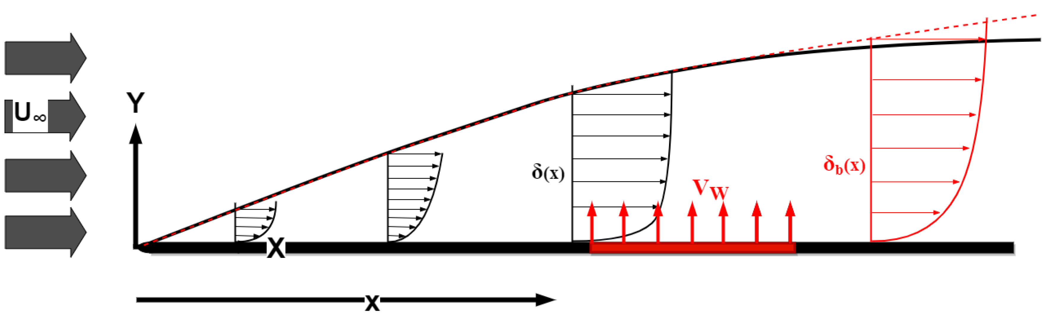
Figure 2.
Law-of-the-wall representation of a TBL profile using inner length scales where viscous sub-layer and logarithmic layer is presented with Equation-1 and Equation-2 respectively [5].
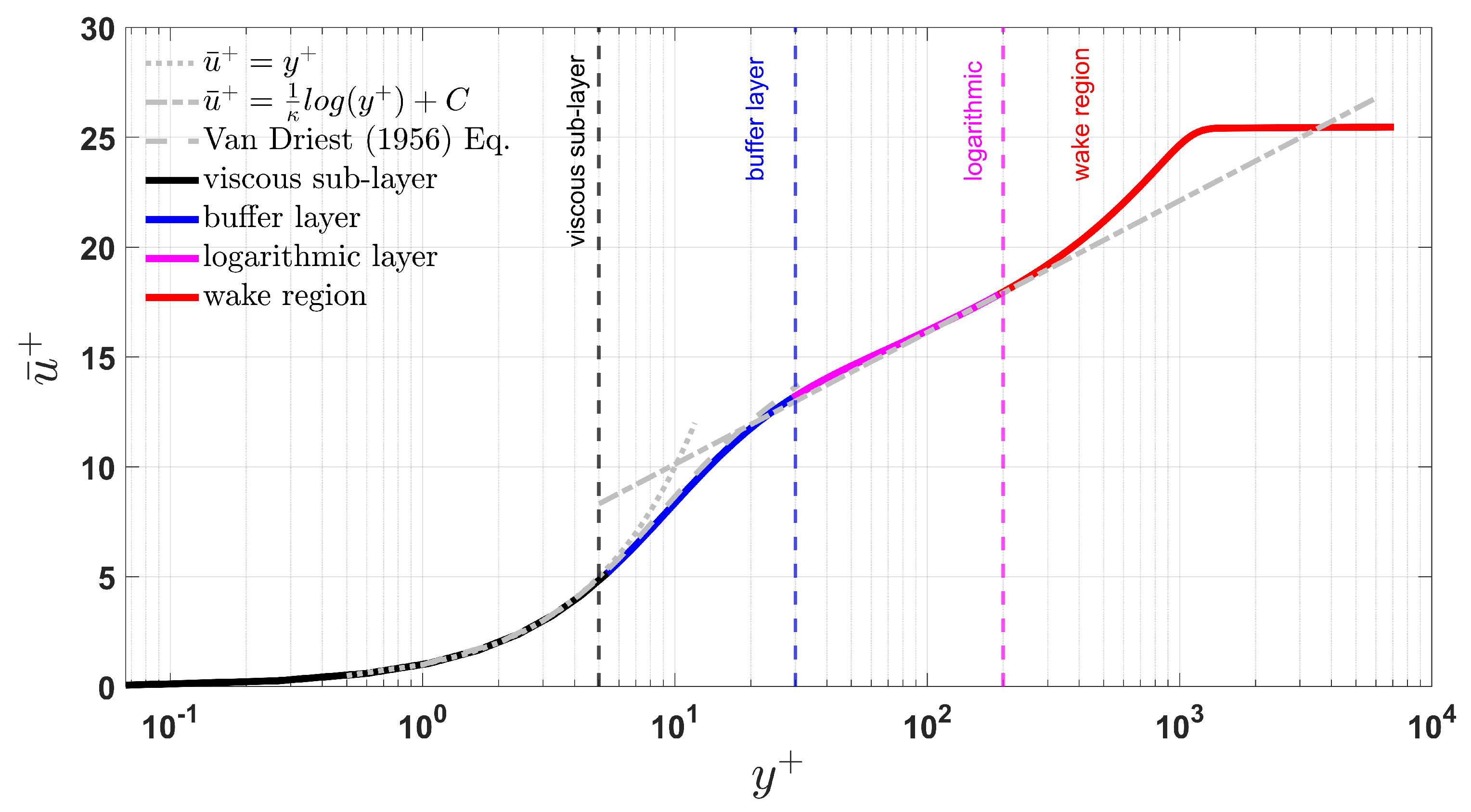
Figure 3.
Flow visualization over smooth surface TBL in the FOV as indicated in Figure 11 at using PIV images; (b) Flow visualization over perforated surface with uniform blowing at 0.7%; the vertical arrow indicate the boundary layer thickness and flow is coming from right to left from readers reference for both (a) and (b) [5].
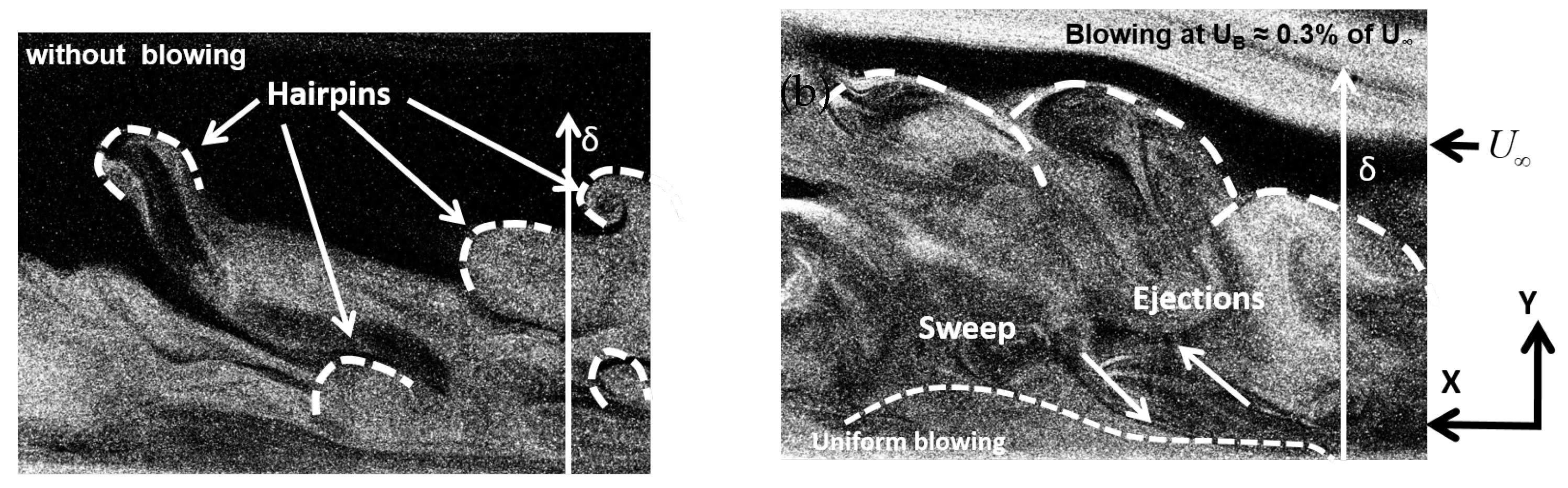
Figure 4.
Schematic of the flat plate setup: (a) xz projection (top view), blowing area indicated in white; (b) xy projection (side view); and (c) microscopic image of the perforated wall with staggered hole arrangement and (d) xy projection of an individual hole.
Figure 4.
Schematic of the flat plate setup: (a) xz projection (top view), blowing area indicated in white; (b) xy projection (side view); and (c) microscopic image of the perforated wall with staggered hole arrangement and (d) xy projection of an individual hole.
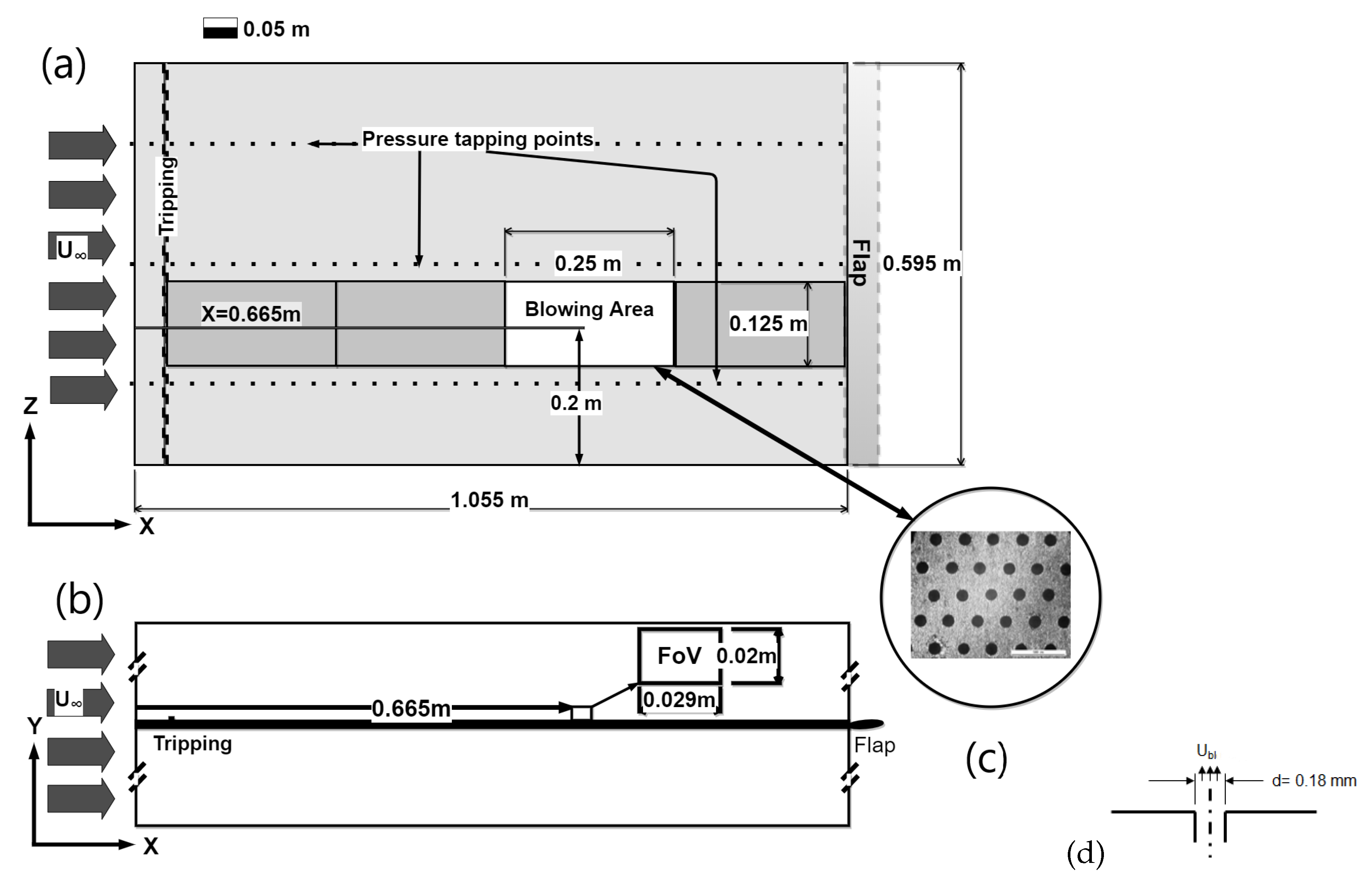
Figure 5.
(a) Photograph showing the PIV setup at BTU wind tunnel, (b) Isometric schematic of the optics and PIV system, (c) FOV dimension with resolved velocity vectors.
Figure 5.
(a) Photograph showing the PIV setup at BTU wind tunnel, (b) Isometric schematic of the optics and PIV system, (c) FOV dimension with resolved velocity vectors.
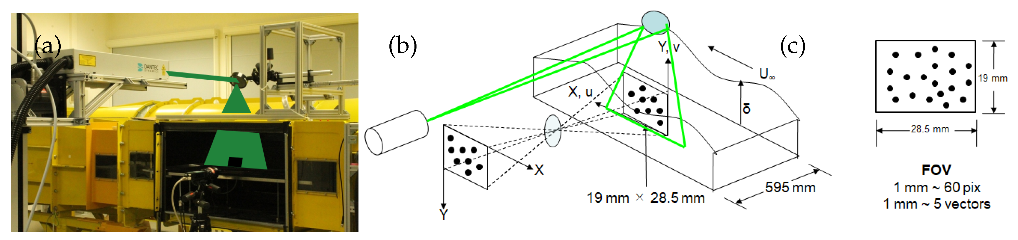
Figure 6.
Mean streamwise velocity profile at obtained using PIV, LDA and HWA, (a) Outer scaled, (b) Law-of-wall presentation.
Figure 6.
Mean streamwise velocity profile at obtained using PIV, LDA and HWA, (a) Outer scaled, (b) Law-of-wall presentation.
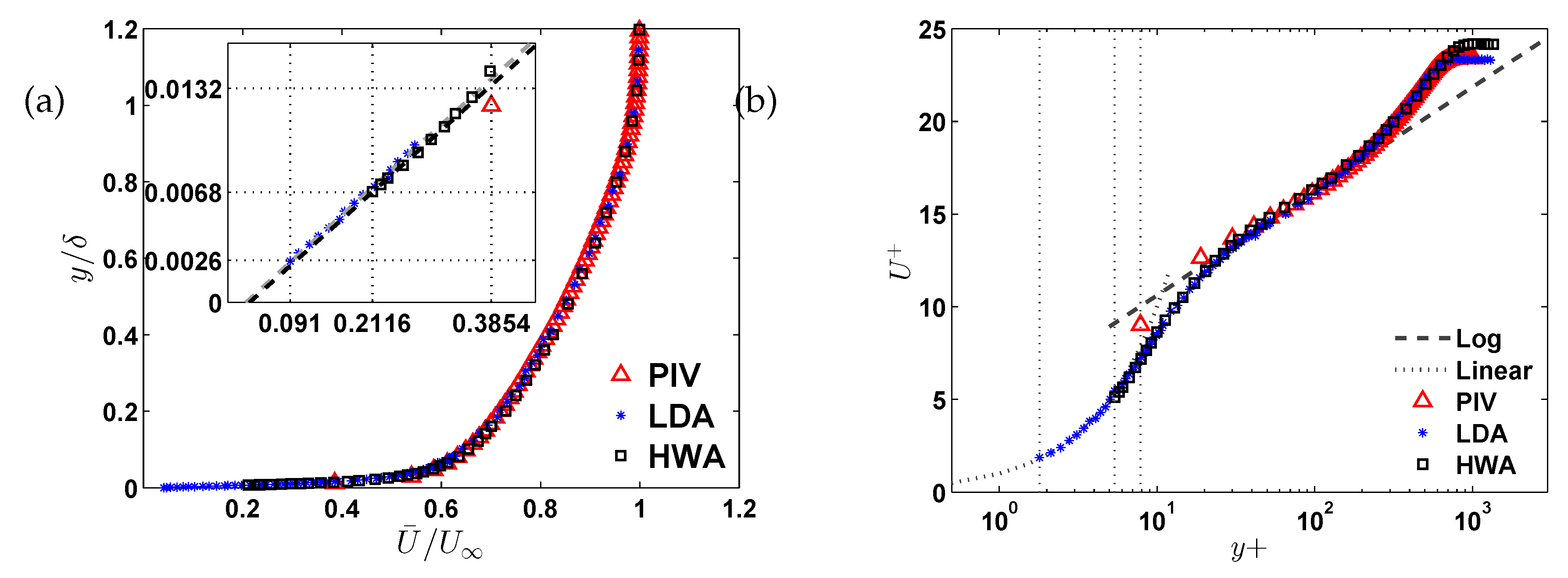
Figure 7.
Mean streamwise () and wall-normal () fluctuation profiles at obtained using PIV, LDA and HWA, (a) presentation using outer scaling parameters; (b) inner scaling parameters.
Figure 7.
Mean streamwise () and wall-normal () fluctuation profiles at obtained using PIV, LDA and HWA, (a) presentation using outer scaling parameters; (b) inner scaling parameters.
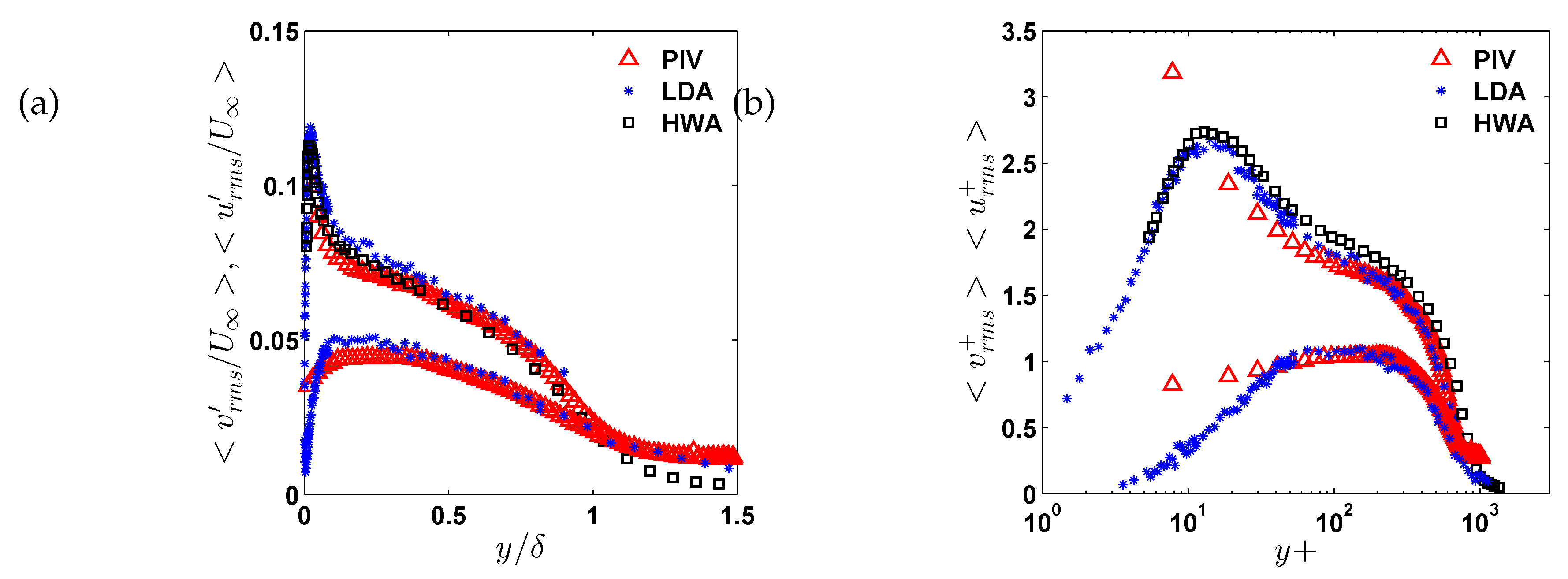
Figure 8.
Skewness and flatness profiles of streamwise velocity obtained using PIV, LDA and HWA using inner scaling parameters, (a) Skewness; (b) Flatness
Figure 8.
Skewness and flatness profiles of streamwise velocity obtained using PIV, LDA and HWA using inner scaling parameters, (a) Skewness; (b) Flatness
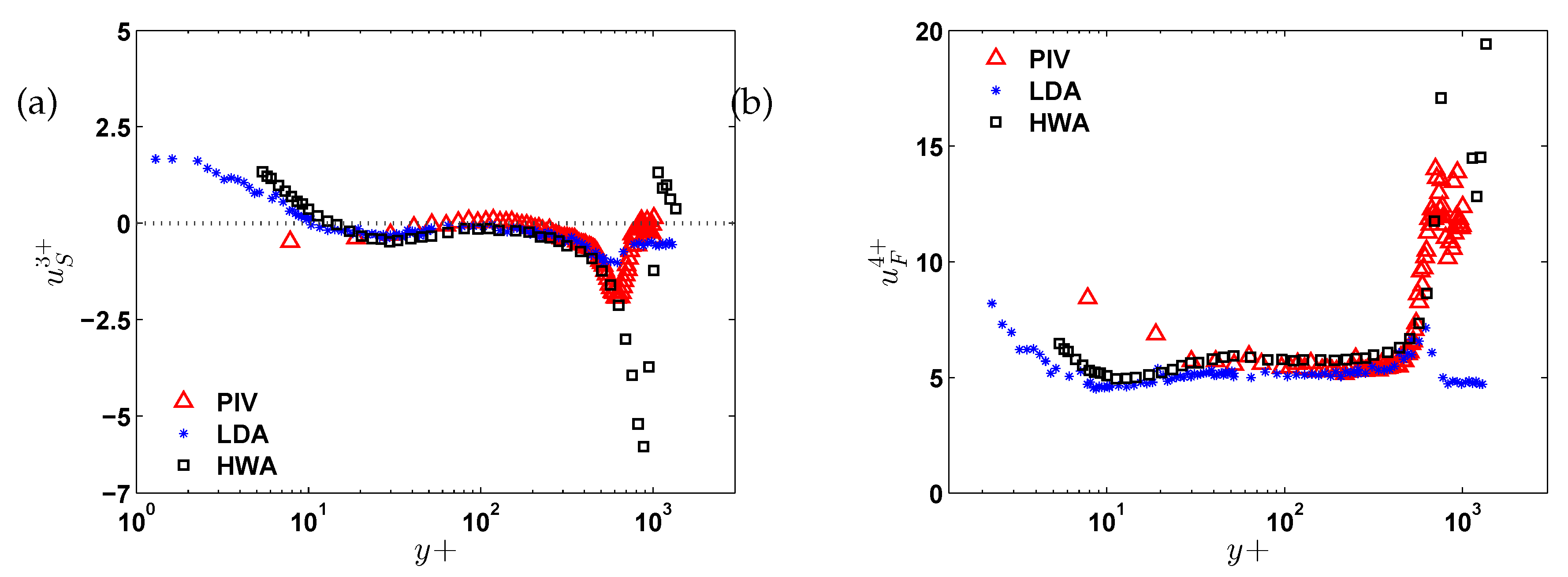
Figure 9.
Mean and rms profile of streamwise velocity along the wall distance for SBL cases obtained using PIV, LDA and DNS, (a) Mean streamwise velocity profiles (b) RMS profiles of streamwise and wall-normal fluctuations.
Figure 9.
Mean and rms profile of streamwise velocity along the wall distance for SBL cases obtained using PIV, LDA and DNS, (a) Mean streamwise velocity profiles (b) RMS profiles of streamwise and wall-normal fluctuations.
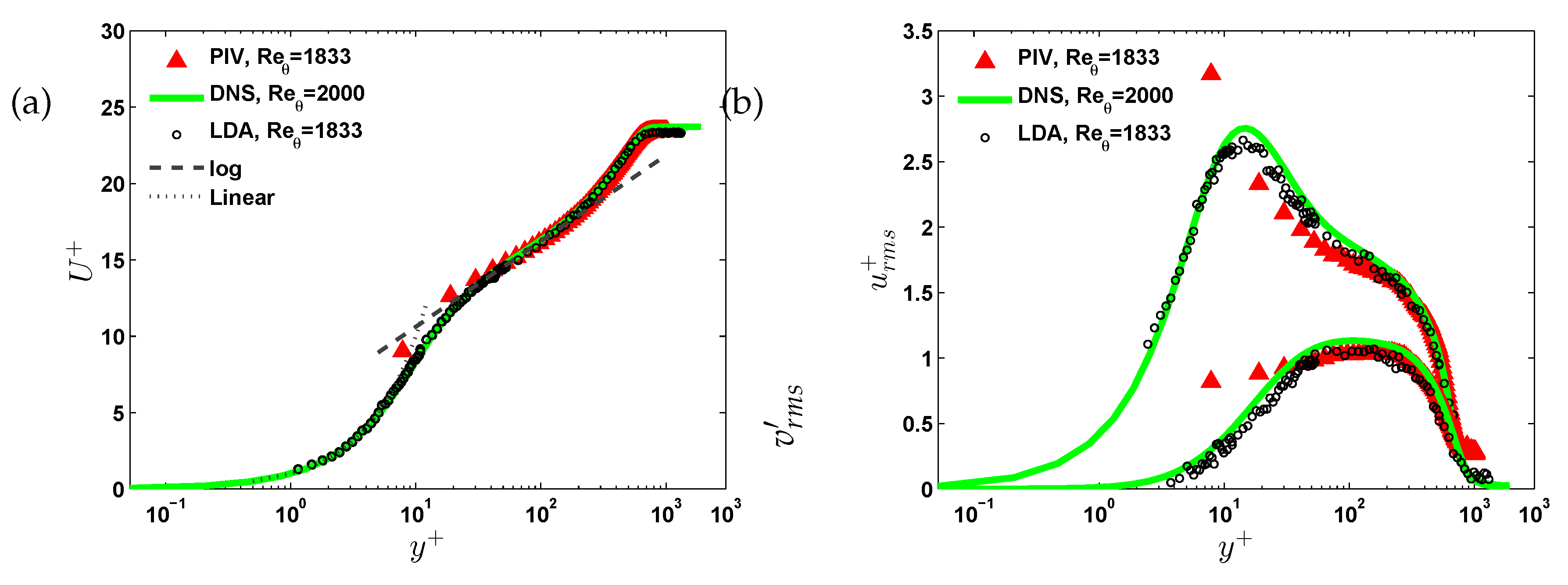
Figure 13.
Spatial development of the TBL downstream stations along the flat plate, comparing SBL and UB, (a) spatial development of dimensional [m], where, SBL is indicated with ’– –’ and UB at blowing ratio, F = 0.85% is indicated with ’– –’, (b) Increase in in percentage of cases.
Figure 13.
Spatial development of the TBL downstream stations along the flat plate, comparing SBL and UB, (a) spatial development of dimensional [m], where, SBL is indicated with ’– –’ and UB at blowing ratio, F = 0.85% is indicated with ’– –’, (b) Increase in in percentage of cases.
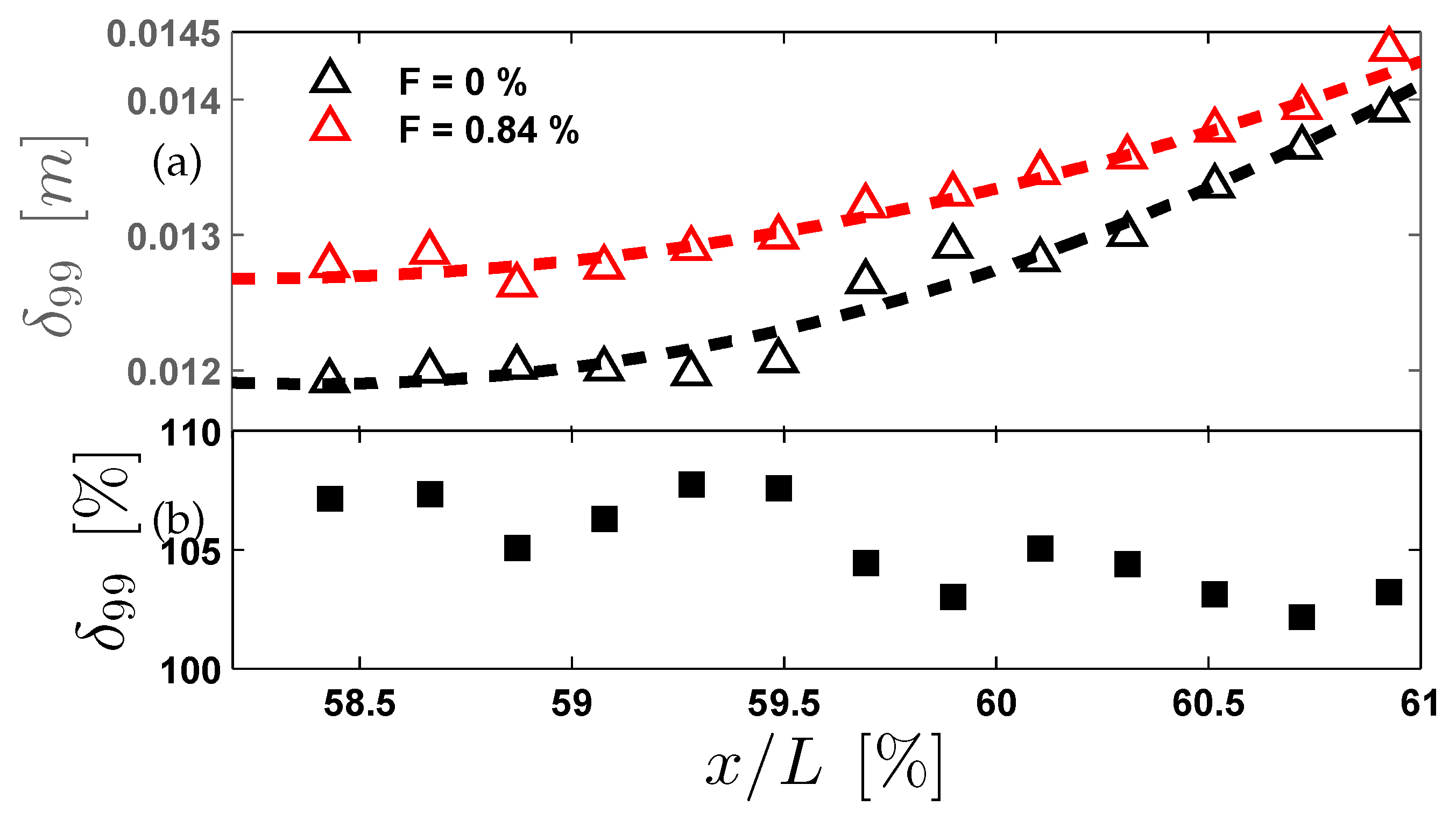
Figure 14.
Probability distribution function of the velocity components along outer-scaled wall-distance, (a) of SBL, (b) of UB at F=0.85%, (c) of SBL and (d) of UB at F=0.85%.
Figure 14.
Probability distribution function of the velocity components along outer-scaled wall-distance, (a) of SBL, (b) of UB at F=0.85%, (c) of SBL and (d) of UB at F=0.85%.
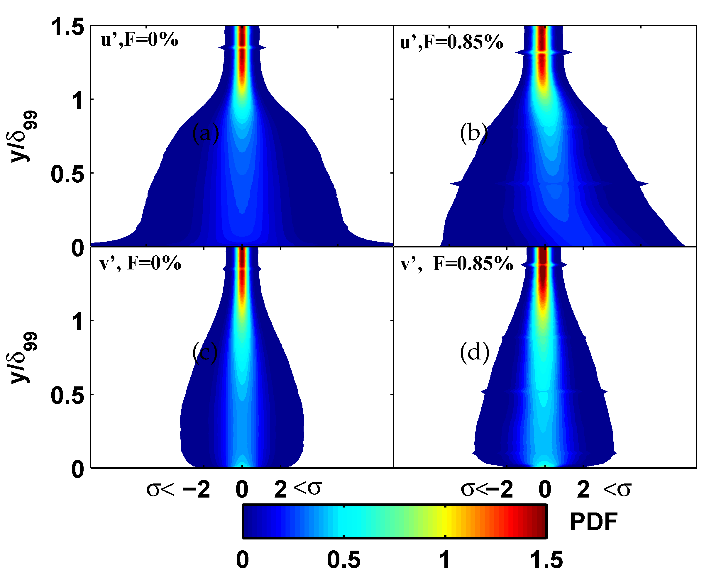
Figure 15.
Reynolds stress profiles () comparing PIV measurements with reference datasets, (a) DNS data from [25] at (left), (b) HWA data from [23] at (right). Empty triangles denote PIV data (: SBL; : UB at ).
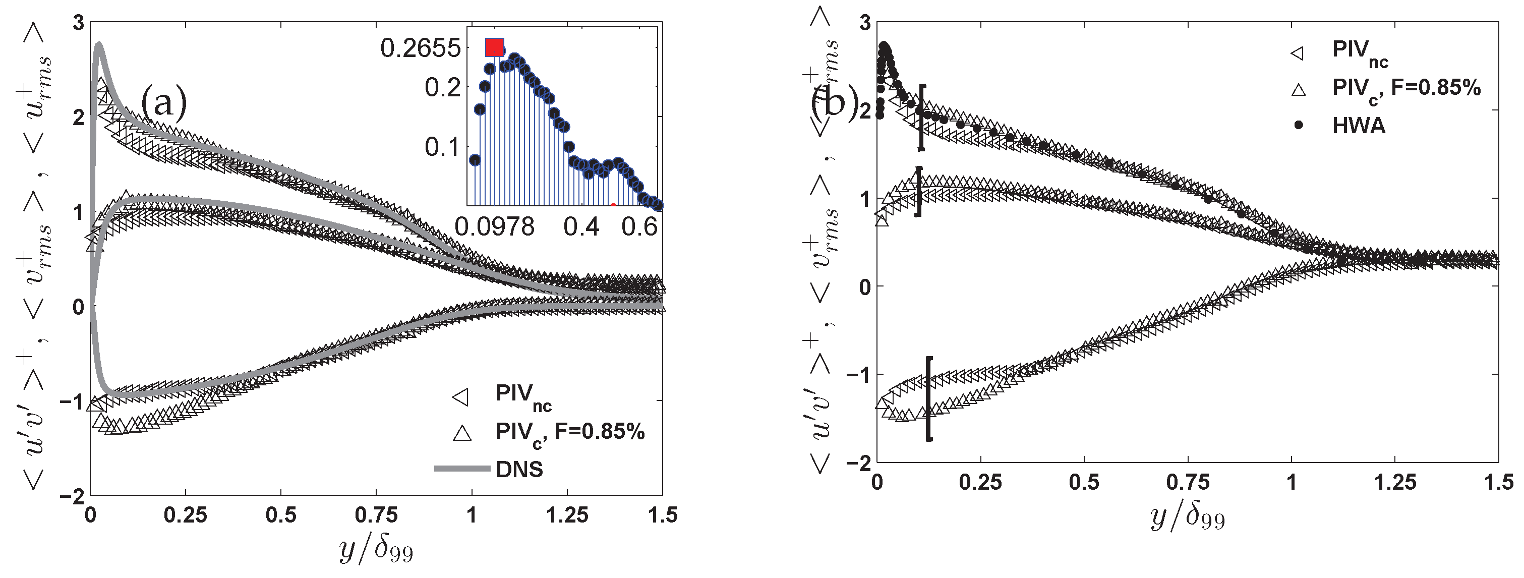
Table 1.
Selection of measurement techniques for flow control assessment
| Technique | Key Insights | Strengths | Limitations |
|---|---|---|---|
| PIV | Visualizes large-scale velocity fields and coherent structures; shows redistribution of turbulence | Good spatial coverage; global flow visualization | Limited temporal resolution; less effective for rapid near-wall fluctuations |
| LDA | Provides high-resolution pointwise measurements of mean and fluctuating velocities near the wall | Non-intrusive; accurate local statistics | Point measurements only; no spatial flow field |
| HWA | Offers detailed, time-resolved turbulence statistics; sensitive to near-wall effects | Exceptional temporal resolution; captures rapid fluctuations | Intrusive; possible probe interference; limited spatial domain |
Disclaimer/Publisher’s Note: The statements, opinions and data contained in all publications are solely those of the individual author(s) and contributor(s) and not of MDPI and/or the editor(s). MDPI and/or the editor(s) disclaim responsibility for any injury to people or property resulting from any ideas, methods, instructions or products referred to in the content. |
© 2025 by the authors. Licensee MDPI, Basel, Switzerland. This article is an open access article distributed under the terms and conditions of the Creative Commons Attribution (CC BY) license (http://creativecommons.org/licenses/by/4.0/).
Copyright: This open access article is published under a Creative Commons CC BY 4.0 license, which permit the free download, distribution, and reuse, provided that the author and preprint are cited in any reuse.


