Submitted:
05 July 2025
Posted:
07 July 2025
Read the latest preprint version here
Abstract
Trust in machine learning models by domain experts and end users is essential for model deployment by them, particularly in high-stakes fields such as healthcare diagnosis. However, consistently quantifying model trust across diverse types of ML models is a difficult challenge in machine learning. Existing trust concepts often are narrow in scope and are not clearly defined for computing a trust score. This paper introduces a new concept of model sureness, which is a quantifiable and generalizable measure of one of the aspects of trust in ML models. To measure this model sureness a process that combines iterative supervised learning and visual knowledge discovery is proposed. It reduces required training data while preserving model accuracy as conducted case studies demonstrate. The method iteratively varies the training dataset and retrains models until a predefined efficiency criterion is met. The measure of the model sureness is defined as a ratio of the number of successful iterations to the total number of iterations. The models with higher ratio of eliminated cases are defined as having higher sureness measures. Case studies across three standard datasets from biology, medicine, and handwriting recognition are conducted. These demonstrate that the method can preserve model accuracy and eliminate 20% to 80% of noisy or redundant instances, with an average reduction of around 50%.
Keywords:
Model Sureness
; Iterative Supervised Learning
; Visual Knowledge Discovery
1. Introduction
1.1. Motivation
Trust in machine learning (ML) models by domain experts and users is critical for deployment of models by them [1]. Trust involves more than just accuracy — it includes the user’s confidence in a model’s accuracy, personal comfort with understanding it, and willingness to let the model make decisions [2,3]. Trust is commonly associated with the stability of the model’s form (pattern) and its predictive accuracy under multiple variations. These variations include changes to training data, types of noise, learning algorithm parameters, models explanations, and others. Although many concepts of ML model trust have been proposed, this paper expands on them by introducing Model Sureness (MS).
Specifically, our model sureness concept is to measure the impact of training data variations on model accuracy for a chosen algorithm. Consider an algorithm that builds high-accuracy models even when trained on significantly varied training data. Then we call these models of high training data model sureness, a prerequisite for the model to be of high trust [4]. Model sureness measures in response to variations beyond training data are beyond the scope of this study.
We define model sureness using Iterative Supervised Learning (ISL) and Visual Knowledge Discovery (VKD) processes, identified later. If a much smaller subset of training data can be used to discover a model that yields the same properties as the one trained on the full known dataset, then this model would be considered to have high model sureness. See Figure 1 for 2-D examples that illustrate both low-risk and high-risk classification scenarios, each reflecting different levels of model sureness. Removing many cases in (a) will still allow us to build the model with the same high accuracy.
Commonly, noise in data obscures patterns and decreases model accuracy. We aim to discover models with stable accuracy despite possible noise. Iteratively analyzing how adding or removing cases affects model accuracy can help identify the smallest subsets of training data required for reliable performance. However, the order in which cases are added or removed significantly impacts resultant models. Exhaustively testing all possible case combinations would be combinatorially infeasible. To decrease computations and preserve class balance we use stratified sampling repeatedly in exploration of plausible scenarios. As a result, the process is stochastic through experimental repetitions.
Noisy cases in training data are often associated with non-representative patterns that obscure meaningful structure. In some of our case studies, the process eliminated from 20% up to 80% of such noisy or redundant cases with around 50% of cases being eliminated on average.
The benefit of this approach is not only in reducing data volume, but in identifying which cases are truly representative for building the model. This method is conceptually aligned with [5], which identified worst-case training instances via a visual knowledge discovery process.
Discovering such truly representative data by visual means often enhances purely analytical approaches [6,7,8]. While cutting down the number of training cases is especially relevant for large datasets, such as the MNIST handwritten digit dataset, which contains 60,000 training instances in a 784-D space. Case study 3.3 examines this scenario showing that models can be discovered with comparable accuracy extracted from only 9,600 cases instead of 60,000 cases resulting in substantial computational benefits.
Reducing the number of training cases may not always be successful. A significant decrease in accuracy after removing some training cases implies that these cases are strongly representative of its class or play a key role in revealing class patterns.
We can assess impactful cases through visual inspection in a lossless visualization by comparing them to their nearest neighbors that are not so impactful. Conversely, if model accuracy remains largely unaffected by the removal or addition of selected cases, those cases are likely not representative of the most representative class structure or even can represent noise.
In general, we can vary any characteristic in the model construction pipelines—such as attributes, parameters, and other design choices—and measure model stability for them as one of the model trust indicators. For instance, this process can identify a stable and relevant subset of data attributes. Moreover, trust in a model depends on the assumptions made during its construction. Unfortunately, users are rarely aware of these assumptions, yet in high-risk domains like healthcare diagnosis, such assumptions require critical scrutiny.
The common ML assumption that the distribution of unseen data will match the training data distribution limits potential deployment in trust-critical applications. This assumption, while potentially reasonable at the population level, fails to account for the case-specific variances and outliers. This is especially important for high-stakes tasks, where the cost of error from a single case can be significant. Crucially, we cannot assume all possible data instances are known or that new outlier cases will not emerge. Research shows that atypical cases behave fundamentally differently and can disproportionately impact model performance compared to typical cases [5]. The proposed model sureness measure helps to test the assumptions of distributional similarity between training and unseen data. Formally, it enables mathematical bounds of the minimum and maximum training data size required to achieve desired model properties like accuracy.
The proposed BASL process allows for dataset reduction for multiple ML algorithms. One of the examples is the generalized iterative classifiers (GIC) [6,9]. These models use generalized decision trees (GDTs), which allow for non-binary decision levels. Because each GDT level depends on the structure and composition of the training data, reducing the dataset has a cascading effect, simplifying downstream decision nodes and improving model interpretability.
1.2. Background Concepts
Background concepts for this study are from two domains: (1) active learning [10] and (2) visual knowledge discovery through lossless visualization of multidimensional (n-D) data [7].
Active Learning (AL) proceeds in a forward direction by querying an “oracle” or teacher to label new data points for building improved models. In this setting, Iterative Supervised Learning (ISL) is used to iteratively expand the training data to optimize model accuracy [10,11,12]. The optimization efficiency criteria vary with implementation and task. However, the efficiency of this querying process is usually measured by how many labeled cases are required to reach the desired accuracy. While our model sureness measure builds on this idea it extends it in both scope and direction.
In evaluating model sureness visual knowledge discovery can be used to discover ML models along with traditional pure computational ML algorithms and (2) to visualize multidimensional data losslessly to analyze these data and ML models build on them. In visualization, occlusion of data cases can obscure dominant patterns. Separating these occluding cases can reveal clearer structures in the remaining data, enabling identification of more precise patterns using interpretable frameworks such as decision rules based on First Order Logic (FoL), instead of relying on simpler approaches like decision trees (DT) or models built only from individual attributes [9]. This two-step process allows one to observe and analyze how patterns and models dynamically change as training data size is increased or decreased.
Alternative model sureness measures have been proposed for specific domains such as network security and quantum computations [13,14,15], where they focus on uncertainty or repeatability within limited ML contexts. The proposed Model Sureness (MS) measure complements the traditional Model Confidence measure, which provides a statistical confidence interval (CI) for individual predictions [16]. Using model sureness provides a more complete characterization of model trust. To compute MS, we iteratively grow or shrink the training data, retraining models each time. This process evaluates the stability of model accuracy under data variations. MS is then quantified as the ratio of the number of stable models—those maintaining a target accuracy threshold—to the total number of iterations that produced models. The central goal is to determine how reliably an ML model maintains accuracy and form of the model as the training data changes.
We formalize this bidirectional process of adding or removing data as Bidirectional Active Supervised Learning (BASL) process. Unlike standard Active Learning, BASL can operate without querying an oracle or teacher, enabling exploration of data sufficiency when all labels are assumed available.
BASL assumes the availability of a sufficiently labeled dataset. This assumption is increasingly practical due to advances in ML-driven synthetic data generation, reducing reliance on manual annotation while preserving essential model properties like accuracy [17,18]. Since manual data labeling is both computationally expensive and labor intensive it would prevent these methods from being fully utilized.
Given the assumption of ample labeled data, BASL seeks to identify the smallest subset of training examples needed to still capture the dominant patterns necessary for a supervised ML classifier to learn effectively. Such a reduction of ML training dataset size has multiple benefits with a few important ones listed below:
(1) Simplified analysis. For example, we can get 8 times less data as our experiments show. This enables visual explanations of the model prediction to be feasible for a wider set of ML tasks with less occlusion. This includes lossless visualization of similar cases to a new case to be predicted.
(2) Lower computational cost. For example, finding k nearest neighbors (k-NN) of a given case can be computed approximately 8 times faster on the dataset reduced by the same factor. In an experiment with k-NN, a 20% reduction in data size resulted in a 5 times speed-up on benchmark data.
(3) Improved deployment efficiency. Reducing data redundancy conserves memory and compute resources, which is especially important for edge devices like mobile, Internet of Things (IoT), and microcontroller platforms.
1.3. Relation to VC Dimension
In ML it is known that the amount of data needed to train an accurate prediction model is highly dependent on the data complexity [19]. Thus, measures and bounds of this exist for quantifying this issue such as the Vapnik–Chervonenkis dimension (VC-dim) [20]. VC-dim measures the size of a dataset that a given algorithm can classify correctly. The data size is defined by a positive integer pair (n, m), where n is the space dimension (n-D space), and m is the number of cases/n-D points in the dataset. However, the methods to measure this complexity are mostly theoretical, and not well-defined outside of either very generalized cases or specific scenarios [19,20,21]. Instead, more well-defined bounds exist that have been mathematically proven, particularly for upper bounds [19,22,23].
Applying the VC-dimension to binary classification algorithms finds a threshold value m (case count) for a classifier working in each dimension n to classify/“shatter” any n-D dataset without classification errors [19,20,23]. For example, a linear classifier in 2-D space can classify without any error only three arbitrary 2-D points, thus here we have a pair of (n, m) = (2, 3) [19,20,24]. In other words, a linear classifier cannot guarantee that with any arbitrary 4 or more 2-D points it will correctly classify all these arbitrary 2-D points. Note that for some, not all, datasets with m > 3 it is possible with a linear classifier.
Therefore, the practical value of the pair (2, 3) is very limited for real world ML tasks because all real datasets contain many more cases than just three with instead hundreds, or thousands of them, with very different mutual relations between them. Thus, by the VC-dim all these variable small and large datasets are within the same risk category of misclassification. However, it is intuitive that these risk categories are not the same for different datasets. Figure 2 shows this where the addition of one data case makes an easy classification task much more difficult. Here a single case requires relearning the model’s discriminant line and deteriorates the classification margin. This drastically lowers the model sureness on these data.
The key idea of the VC-dim is to find the capacity of a specific ML algorithm A in terms of a pair <n, m>. It is answering the question: “Will the algorithm A be able to classify a set of m cases (n-D points) for all possible split these m cases to k classes?” For example, if we have only two classes k = 2 then the question is: “Will the algorithm A be able to correctly classify any m cases in n-D space and any possible split of these cases to two classes?” Thus, VC-dim measures the capabilities of the algorithm to classify all possible datasets of a given size (n, m).
Respectively, the key application of the VC-dim is to check if an algorithm for the given number of cases m and classes k will be able to classify any n-D data or not. In most cases VC-dim exaggerates the requirements on the algorithm to be able to classify cases for a given dataset, because it checks any possible split of these cases to classes. However, in practice, many ML algorithms operate under an informal data compactness hypothesis that limits split sets. Under the compactness hypothesis, the cases of a single class are located nearby forming blobs. It is also assumed that these blobs form constellations that are separable by linear or non-linear functions. This is a fundamental idea behind various kernel-based algorithms like SVM.
The difference in our approach from VC-dim is illustrated by the following example. Consider m n-D points (C1, C2, …, Cm,) and 2 classes. There are multiple possible splits of these m cases to two classes, such as: (C1) is split from (C2, C3, …, Cm), or (C2) is split from the rest of the cases (C1, C3, …, Cm), or (C1, C2) are split from the remaining (C3, C4, …, Cm), and so on. VC-dimension deals with combinatorics of all possible splits of m n-D points for a given classifier algorithm. In contrast, our model sureness measure deals with this combinatorics of subsets of a single actual split of m n-D points of the given training data for a given classifier algorithm. Moreover, our model sureness measure deals with splits, where a single n-D can represent cases of two or more classes, which is known to often happen in real training data.
1.4. Relation to Other Relevant Concepts
This section considers the relation of our model sureness measure to other relevant concepts. Below, as above, we assume the data size is defined as (n, m) pair, where n is the dimension of the data points and m is the number of n-D points. Many modifications of the VC-dim exist. They enable rigorous analysis beyond binary classification, such as in multi-class learning, regression, and dynamical systems [24] within a pure computational approach and a general concept of the VC-dim presented above with all possible (n, m) datasets. Some approaches abstract the VC-dim problem to a set-theory perspective [22] or focus on its pure geometric interpretation [23].
The approach in this paper differs from them by dealing with a single training dataset and its subsets, which is not bound by VC-dim defined for all (n, m) datasets. Next, we follow the approach that blends computational analysis with visualization [25] to verify, analyze, and expedite computational discovery of the minimal ML training datasets.
This includes support to set up (1) model hypothesis space, (2) a stopping criterion for changing training data, and (3) model and its interpretation verification. It became possible because the user can visualize the subsets of data where less occlusion is present, allowing for better understanding of the shape of the data classes. Specifically, the use of lossless visualization on multidimensional data in General Line Coordinates [7,8] allows us to conduct it more completely due to preservation of all multidimensional information in contrast with common dimension reduction methods like PCA, MDS, and t-SNE.
This visualization also allows measuring better model’s accuracy in contrast with a standard “blind” k-fold CV (cross-validation) approach. The CV approach is considered “blind” because it only randomly selects validation cases and can exaggerate the accuracy, because the worst subsets may not ever get selected [5]. We expand on the k-fold CV by running much more times than the usual 10 times (10-fold CV) to mitigate it. Moreover, the process may be seeded by an oracle. This allows for learning a complex metric which is specific to a given classification task.
Relation to well- and ill-posed problems. A problem is well-posed if it satisfies the following conditions (as defined by Hadamard [26]): (1) Existence: A solution exists, (2) Uniqueness: The solution is unique, and (3) Stability: Small changes in input lead to small changes in output). If any of these conditions fail, the problem is considered ill-posed. Typically, ML problems are ill-posed with their solutions (models) violating at least one or more of these conditions. The proposed model sureness measure is to measure the uniqueness and stability of the ML models relative to variations of training data allowing us to judge how well- or ill-posed the problem is.
The rest of this paper is organized as follows. Section 2 details Methodology with Definitions and Algorithms. Section 3 details Case studies with Fisher Iris, Wisconsin Breast Cancer, and MNIST Digits datasets. Section 4 contains a Discussion, followed by section 5 of Conclusion and Future Work. After this are supplementary materials, links to developed open-source software implementations, followed by the cited references.
2. Methodology
2.1. General Framework
To study ML model sureness, we work with subsets of labeled data modified over many iterations with an ML model rebuilt each iteration to analyze and respond to. We iteratively rebuild the used ML model and observe if we reach stable states of accuracy on either growing or shrinking data subsets over many experimental iterations. As the overall experiment repeats, a minimum and maximum number of cases are averaged, and we check for convergence to an interval bounding the size for a minimal data subset. If interval convergence is not reached, then we can conclude that the chosen ML algorithm is unstable on the given data for the specified accuracy threshold.
This process relies on a selected ML model algorithm and some given dataset. The data may be previously split into train and test subsets like a 70:30 split being 70% to train and 30% to test with. However, some data will come without being split beforehand. For analysis of such data, we must split the data to train and test prior to testing the model sureness. The main process conducted is demonstrated in the Figure 3 flowchart diagram.
2.2. Definitions
This section defines the main concepts that we work with in this paper.
Definition 1. Minimal Necessary Training Subset (MNTS):
A subset Sm from the given dataset S that is sufficient to train an ML model M to achieve the model accuracy at the level or above the threshold T for a given ML algorithm A, e.g., 95% accuracy.
Thus, Sm is a result of some function F, Sm= F(S, M, A, T), that will be discussed later.
Definition 2. Maximal Unnecessary Training Subset (MUTS):
A subset from dataset S after exclusion of the minimal necessary training subset (MNTS) Sm from S: Su = S\Sm.
Definition 3. Minimal Magnitude of Training Subset:
The number of elements |Sm| is the magnitude the minimal necessary training subset (MNTS) Sm.
Definition 4. Model Sureness (MS) Measure:
The Model Sureness Measure U is the ratio of the number of unnecessary n-D points Su: |Su| =|S| - |Sm| to all point is set S,
U = |Su| /|S|
Larger values of U indicate that more unnecessary points can be excluded from the training data to discover a model that satisfies T threshold accuracy. This larger U will also indicate higher trust in the model.
Definition 5.
Model Sureness Lower Bound (MSLB):
It is a number LB that is not greater than Model Sureness measure U: 0 < LB ≤ U.
Definition 6.
Tight Model Sureness Lower Bound (TMSLB):
It is a Lower bound LBT is such that U- LBT ≤ ε, where ε is allowed difference between U and LBT.
Definition 7.
Model Sureness Upper Bound (MSUB):
Is a number LUB that is no less than Model Sureness measure U: 1 > LUB ≥ U.
Definition 8.
Tight Model Sureness Upper Bound (TMSUB):
Is a number LTU such that LTU - U ≤ ε, where ε is an allowed difference of U and LTU.
Definition 9. Upper Bound Minimal Training Subset:
The subset SUB of n-D points from set S needed to produce a model with Model Sureness Upper Bound LTU.
For a practical reason we often search only for an Upper Bound Minimal Training Subset SUB with its Model Sureness Upper Bound LUB. Computationally finding the actual model sureness measure value, or its bounds, can lead to exhaustive search of computing models produced by the algorithm A on multiple subsets of the set S. The number of those model computations NMC and complexity of each model computation CMC depend on the algorithm A, a dataset S, and threshold T for the model accuracy that is set. Respectively, we define these concepts below.
Definition 10.
The number of times that algorithm A computes models {M} on subsets of dataset S is denoted as NMC.
Definition 11. The complexity of each model computation
CMC by an algorithm A on a subset SRi of set S is denoted as CMC(SRi).
Definition 12. The total complexity of all model computation
TMC by an algorithm A on all selected subsets {SRi} of set S is denoted as TMC(S) and it is a sum of all CMC(SRi):
Here we do not specify details of complexity of model computation CMC(SRi) by an algorithm A because it heavily depends on the algorithm A. For instance, these details are very different for DTs, k-NN, SVM, neural networks, and others. Respectively, it is then specified when the algorithm A is selected.
At first glance the computational complexity is not important for the user as long as it takes a reasonable time to compute the model sureness measure. However, it is truly important for a user. Consider two algorithms A1 and A2 with the same model sureness measure, say, 0.8, where algorithm A1 requires two times less time than algorithm A2, to compute its model sureness measure because A2 is more complex than A1. Therefore, a user would prefer algorithm A1 because it is simpler with the same model sureness. This is under the assumption that both algorithms are interpretable at the same level.
Many ML algorithms have stochastic components leading to different accuracies and different times to produce the model. To accommodate this, we use standard deviations of accuracy and the number of cases in the minimal set.
2.3. Algorithms
The algorithms for computing the model sureness measure run many times over to analyze different subset selections. Below we present ways to formalize subsets selection methods that involve random stratified sampling and a human-guided visual selection sampling method. We also visualize the results of iterations where the accuracy threshold is reached and those where it is not reached. In both situations we get a visual sense of the dominant patterns to use in model building and/or to improve them.
-
Minimal Dataset Search (MDS) Algorithm: It is characterized by as a triplet of:<BDIR, T, IMAX>Here BDIR is a computation direction indicator bit. BDIR = 0 if the Minimal Dataset Search algorithm starts from the full set of n-D points S and excludes some n-D points from S. Bit BDIR = 0 if the Minimal Dataset Search algorithm starts from some subset of set S and includes more n-D points from set S. The accuracy threshold T is some numerical percentage value 0 to 1, e.g., 0.95 for 95%. A predefined max number of iterations to produce subsets is denoted as IMAX. This algorithm: (1) reads the triple <BDIR, T, IMAX>, (2) updates and tests the selected training dataset using the respective IMDS, EMDS, and AHSG algorithms, described below.
- Inclusion Minimal Dataset Search (IMDS) Algorithm: It iteratively includes a fixed percentage of n-D points of the initial dataset S to the learnt subset Si, trains a selected ML classifier A thereon, and evaluates accuracy on all known separate test data Sev. It iterates until all data are added and assessed when reaching threshold T, e.g., 95% accuracy of model.
- Exclusion Minimal Dataset Search (EMDS) Algorithm: In contrast with the above Inclusion Minimal Dataset Search, this algorithm instead starts on the entire training dataset S and excludes data iteratively to retrain a selected ML algorithm on. It also assesses reaching the threshold T.
- Additive Hyperblock Grower (AHG) Algorithm: It iteratively adds data subsets to the training data, builds hyperblocks (hyperrectangles) thereon using the existing IMHyper algorithm [27], then tests class purity of each hyperblock iteration on the next data subset to be added.
3. Case Studies
This section presents case studies using the Fisher Iris, Wisconsin Breast Cancer, and MNIST datasets, including experimental results, their interpretation, and conclusions
3.1. Fisher Iris Data Cases Study
This case study is based on the Fisher Iris dataset with an SVM algorithm. Results show that data may be reduced to 61.4% - 77.4% while preserving accuracy when ran independently across 10 independent tests. With 100 tests the results are almost identical, see Table 1. This shows that we need much less than half of this dataset to adequately classify data with the chosen SVM algorithm. Incremental data size was set at 10 cases; the accuracy threshold was 0.95 (95%) with 70:30 data split to training and validation data.
Figure 3 shows the visualization in Parallel Coordinates (PC) of increasing subsets of data used in these experiments to visually analyze the results to the model over iterations. This visualization shows the iterative growth of the training data up until the accuracy threshold is reached. Initially, each data class is represented by just a few cases. Over time, as additional instances are incorporated, the space becomes more densely filled, resulting in a relatively uniform n-D density among the cases that delineate the class boundaries. The test data is visualized in the last PC plot for visual comparison.
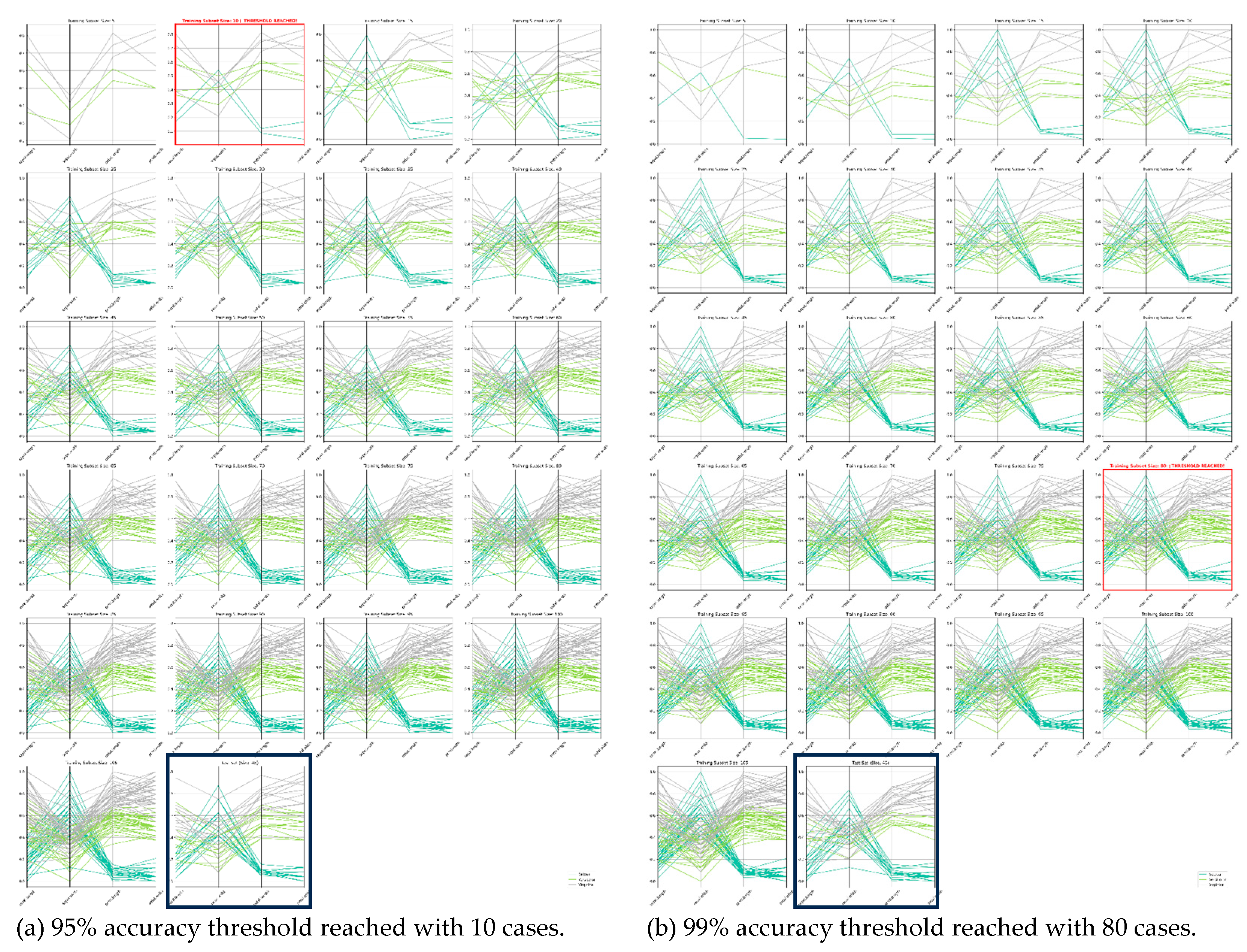
Figure 4.
The increasing subsets of training data with the last subplot showing the test data from experiment presented in Table 1. The red rectangles show the cases which are needed to get 95% accuracy and cases in the black box independently selected cross validation percent of validation data comparison of these rectangles shows high similarity of the datasets in them. We first split data to 70:30 and these 30% are shown in the last subplot in both (a) and (b) and other data are growing to reach 70%.
Table 2 shows the results from this process with Linear Discriminant Analysis (LDA) classifier.
We conducted an experiment with an algorithm from [27] to generate interpretable hyperblocks (hyper-rectangles) as ML classification models. With this approach we can test the hyperblock structures for each iteration on the next data additions. This can demonstrate the robustness of the model in a geometric sense.
In Table 3 the column “Next Misclassified” refers to upcoming cases misclassified when we evaluate the existing hyperblock (HB) built in the former step. For instance, we built a hyperblock with 100 cases of single class. Then we added 10 more cases to the training data with 5 of them that are in this hyperblock, but three of them are not from the class of those 100 cases. These are “next misclassified” cases. While it can happen, in fact, in Table 3, we did not get any “next misclassified” cases.
Each hyperblock (HB) is a simple model, but the number of HBs can be quite large for covering all training data. It is possible that some of these HBs are redundant. One of the algorithms in [27] analyzes it and decreases the number of HBs. The Minimal Dataset Search (MDS) algorithm presented above found a smaller training data subset that is sufficient to get the required accuracy of 95%. It can potentially build a simpler set of HBs than are already built for the whole training data. The actual number of HBs is 2 and the number of HBs for all 70% of training data is 4. It is a minor decrease, but it is still useful to make processing faster without conducting complex optimization.
3.2. Wisconsin Breast Cancer Data Cases Study
This case study follows the same approach as used in section 3.1 above. However, now we use increment size of 20 cases. The best results with WBC data are 96.995% while in all cases studies in this paper we aim for no less than 95% accuracy. This is marginally less than best reported in the prior literature using 10-fold CV, not 70:30 that can be lower, which achieved accuracies of 97.01 – 100% [28,29].

Table 4.
Results of experiments on cancer data adding 20 cases, with 70:30 split, and threshold of 95% accuracy.
Table 4.
Results of experiments on cancer data adding 20 cases, with 70:30 split, and threshold of 95% accuracy.
| Characteristics | Number of iterations of SVM run | |
| 10 | 100 | |
| Mean Cases Needed | 20 | 21 ± 5.2 |
| Min Cases Needed | 20 | 20 |
| Max Cases Needed | 20 | 60 |
| Mean Model Accuracy | 0.975 ± 0.01 | 0.969 ± 0.011 |
| Convergence Rate | 10/10 = 100% | 99/100 = 99% |
3.3. MNIST Digits
This case study uses the MNIST digits dataset for handwriting recognition with k-Nearest Neighbor algorithm and CNN. We first perform dimension reduction (DR) by using edge cropping of 3 pixels on all edges and then average pooling with a 2x2 kernel and stride of 2. We iteratively add 100 cases at a time to the training data and converge to 97.2% accuracy every time. Table 5 and Table 6 and Figure 5 summarize these results. Table 5 shows that only 16% of data (9,600 from 60,000 cases) is needed for 97.2% accuracy with k-NN on 10,000 test cases. This stability of the results of each experiment demonstrates stability of k-NN for MNIST data.
Table 6 shows in detail the distribution of digit class labels in the decreased dataset. It demonstrates that these data are relatively balanced (about 1000 cases per digit class) as it is for the full MNIST dataset itself.
Figure 5 presents visualization of these 9,600 converged cases with k-NN for k = 3 after Dimension Reduction to 121-D from original 784-D revealing more visual patterns.
The results reported in this case study show that we can use a much smaller subset of data for this task even after described dimension reduction and get over 95% accuracy for k-NN with k = 3. Thus, the k-NN algorithm has high sureness on the MNIST data with used k = 3 for this experiment.
So, these data contain little noise and substantial redundancy. The little noise can be a result of a dimension reduction process, which can be tested in an additional experiment with various dimension reduction parameters to validate stability of the used dimension reduction process. The proposed model sureness measure can be expanded from the number of cases m to the changing the dimension n of the cases too. In this way we will get a model sureness for data size pair (m, n).
Below Figure 6 and Figure 7 show the results of model sureness study in PCA and t-SNE visualizations, which despite being lossy can show changes in the data when considering the full data versus the reduced data. Both use the same dimension reduction version of the data. The visualization in Figure 7 allows us to verify if the centers of the data are consistent with the full data, which is essential to maintain consistency of the k-NN classification. Figure 7 confirms that the centroids of the classes are quite similar before and after the data reduction to the stable subset.
Below we present the results of the experiment with CNN on the same MNIST data. We used a CNN model [30] on all 60,000 training cases for 50 epochs and with the same architecture and hyperparameters we get the following test accuracies on all 10,000 test cases presented in Table 7.
The marginal loss of accuracy at only 0.23% testing accuracy with the data after dimension reduction opens an opportunity to conduce model sureness exploration much faster on the reduced dimension. We conducted iterative supervised learning in parallelized processing to find data subsets with 95% accuracy on the same 10,000 test cases. We pick up 100 cases at a time, train the model, evaluate the model on all 10,000 test cases, then repeat until 95% accuracy threshold is reached. See Table 8.
This gives the best model found in 5 trials. This result is reached with only 2,500 training cases instead of the total 60,000 training cases (only 4.17% of the total training cases available). Figure 8 shows plotting these 2,800 cases in Parallel Coordinates.
Figure 8 presented results of plotting the top accuracy tests found for a run that produced 2,800 cases with 95.36% accuracy in Parallel Coordinates.
4. Conclusion
This paper proposes a new model sureness measure for machine learning tasks by combining processes of Iterative Supervised Learning and Visual Knowledge Discovery. It allows us to find smaller and efficient training datasets that allow us to measure the data stability in machine learning models. Furthermore, this allows for validation of selection of data subsets to be explored with human-in-the-loop feedback.
The conducted case studies demonstrate that the training data for ML models can be decreased significantly by eliminating from 20% up to 80% of noisy or redundant cases with around 50% of cases being eliminated on average. This work shows that model sureness is maintained after removing or adding cases by the proposed methods. This simplifies the computational requirements of model training. Moreover, it opens an opportunity for integration with efficient visual methods to deal with noise in the data.
The limitations of the proposed model sureness measure methods are as follows. Combinatorics of all exploration of all possible subsets is not feasible. The current approach with stratified random selection requires extensive computational resources. To expand the model sureness to vary dimensions by different dimension reduction methods also will require additional significant computational resources. The experiment conducted with MNIST data used one specific form of dimension reduction. The current model sureness measure only varies the data size. Varying other characteristics can be beneficial too.
Future work may focus on analyzing the combinatorial issue discussed as limitations with finding efficient solutions. Future work may test different data splits on training and validation data and finding efficient ways to conduct it. Further study of data subsets size that are added or removed will be beneficial too. Exploration of data subsets can be expanded to synthetic data that are similar or complementary to available training and test data when those data are scarce.
Supplementary Materials
All utilized code is available at: https://github.com/CWU-VKD-LAB the project used in these case studies is at: https://github.com/CWU-VKD-LAB/IterativeSurenessTester
Data Availability Statement
This work uses the following publicly available datasets: Fisher Iris, Wisconsin Breast Cancer, and MNIST digits.
References
- Lin H., Han J., Wu P., Wang J., Tu J., Tang H., Zhu L., Machine learning and human-machine trust in healthcare: A systematic survey. CAAI Transactions on Intelligence Technology, 2024. 9(2):286-302. [CrossRef]
- Lipton Z., The mythos of model interpretability: machine learning, interpretability is both important and slippery, Association for Computing Machinery Queue, vol. 16, 2018. pp. 31–57. [CrossRef]
- Rong Y., Leemann T., Nguyen TT, Fiedler L., Qian P., Unhelkar V., Seidel T., Kasneci G., Kasneci E., Towards human-centered explainable ai: A survey of user studies for model explanations. IEEE transactions on pattern analysis and machine intelligence, 2023. 46(4):2104-22. [CrossRef]
- Yin M., Wortman Vaughan J., Wallach H., Understanding the effect of accuracy on trust in machine learning models. Proceedings of the CHI conference on human factors in computing systems, 2019. pp. 1-12. [CrossRef]
- Recaido C., Kovalerchuk B., Visual Explainable Machine Learning for High-Stakes Decision-Making with Worst Case Estimates. In: Data Analysis and Optimization. Springer, 2023. pp. 291-329.
- Williams A., Kovalerchuk B., Boosting of Classification Models with Human-in-the-Loop Computational Visual Knowledge Discovery. In: International Human Computer Interaction Conf, LNAI, vol. 15822, 2025.Springer, pp. 391-412.
- Kovalerchuk B., Visual knowledge discovery and machine learning. Springer, 2018.
- Kovalerchuk B., Nazemi K., Andonie R., Datia N., Bannissi E., editors, Artificial Intelligence and Visualization: Advancing Visual Knowledge Discovery. Springer, 2024.
- Williams A., Kovalerchuk B., High-Dimensional Data Classification in Concentric Coordinates, Internation Visualization, 2025.
- Settles B., From theories to queries: Active learning in practice. Active learning and experimental design workshop, 2011. pp. 1-18. http://proceedings.mlr.press/v16/settles11a/settles11a.pdf.
- Rubens N., Elahi M., Sugiyama M., Kaplan D., editors, Active Learning in Recommender Systems. Recommender Systems Handbook (2 ed.). Springer, 2016.
- Das S., Wong, W., Dietterich T., Fern A., Emmott A., editors, Incorporating Expert Feedback into Active Anomaly Discovery. 16th International Conference on Data Mining. IEEE, 2016. pp. 853–858.
- Whitney HM, Drukker K., Vieceli M., Van Dusen A., de Oliveira M., Abe H., Giger ML, Role of sureness in evaluating AI/CADx: Lesion-based repeatability of machine learning classification performance on breast MRI. Medical Physics, 2024. 51(3):1812-21. [CrossRef]
- Gupta MK, Rybotycki T., Gawron P., On the status of current quantum machine learning software. preprint arXiv:2503.08962, 2025.
- Woodward D., Hobbs M., Gilbertson JA, Cohen N., Uncertainty quantification for trusted machine learning in space system cyber security. IEEE 8th International Conference on Space Mission Challenges for Information Technology, 2021. pp. 38-43.
- Heskes T., Practical confidence and prediction intervals. Advances in neural information processing systems. 1996.
- Williams A., Kovalerchuk B., Synthetic Data Generation and Automated Multidimensional Data Labeling for AI/ML in General and Circular Coordinates, 28th International Conference Information Visualisation. IEEE, 2024. pp. 272-279.
- Nguyen PA, Tran T., Dao T., Dinh M., Doan MH, Nguyen V., Le N., editor, Efficient data annotation by leveraging AI for automated labeling solutions. Innovations and Challenges in Computing, Games, and Data Science. Hershey: IGI Global, 2025. pp. 101–116.
- Mohri, M., Rostamizadeh, A., & Talwalkar, A., Foundations of Machine Learning (2nd ed.). MIT Press, 2018.
- Vapnik, V., Statistical Learning Theory. Wiley, 1998.
- Vapnik V., Izmailov, R., Rethinking statistical learning theory: Learning using statistical invariants. Machine Learning, 2019. 108, pp. 381–423. [CrossRef]
- Wencour, R. S., Dudley, R. M., Some special Vapnik–Chervonenkis classes, Discrete Mathematics, 1981. 33 (3): pp. 313–318. [CrossRef]
- Vapnik V., Chervonenkis A., On the uniform convergence of relative frequencies of events to their probabilities. 2015.
- Blumer A., Ehrenfeucht A., Haussler D., Warmuth M. K., Learnability and the Vapnik–Chervonenkis dimension. Journal of the ACM, 1989. 36 (4): pp. 929–865. [CrossRef]
- Hayes D., Kovalerchuk B., Parallel Coordinates for Discovery of Interpretable Machine Learning Models. Artificial Intelligence and Visualization: Advancing Visual Knowledge Discovery. Springer, 2024. pp. 125-158.
- Hadamard J., Sur les problèmes aux dérivées partielles et leur signification physique. Princeton University Bulletin, 1902.
- Huber L., Kovalerchuk B., Recaido C., Visual knowledge discovery with general line coordinates. Artificial Intelligence and Visualization: Advancing Visual Knowledge Discovery. Springer, 2024. pp. 159-202.
- Neuhaus N., Kovalerchuk B., Interpretable Machine Learning with Boosting by Boolean Algorithm, 8th Intern. Conf. on Informatics, Electronics & Vision & 3rd Intern. Conf. on Imaging, Vision & Pattern Recognition, 2019. 307-311.
- Kovalerchuk B., Neuhaus N., Toward Efficient Automation of Interpretable Machine Learning. International Conference on Big Data, pp. 4933-4940, 978-1-5386-5035-6/18, IEEE, 2018.
- Artley B., MNIST: Keras Simple CNN (99.6%), 2022, https://medium.com/@BrendanArtley/mnist-keras-simple-cnn-99-6-731b624aee7f.
Figure 1.
Examples of how model sureness is affected by data distribution relative to a linear discriminant function. Additionally, it demonstrates that the border areas of the classes have a high influence on the model capabilities.
Figure 1.
Examples of how model sureness is affected by data distribution relative to a linear discriminant function. Additionally, it demonstrates that the border areas of the classes have a high influence on the model capabilities.
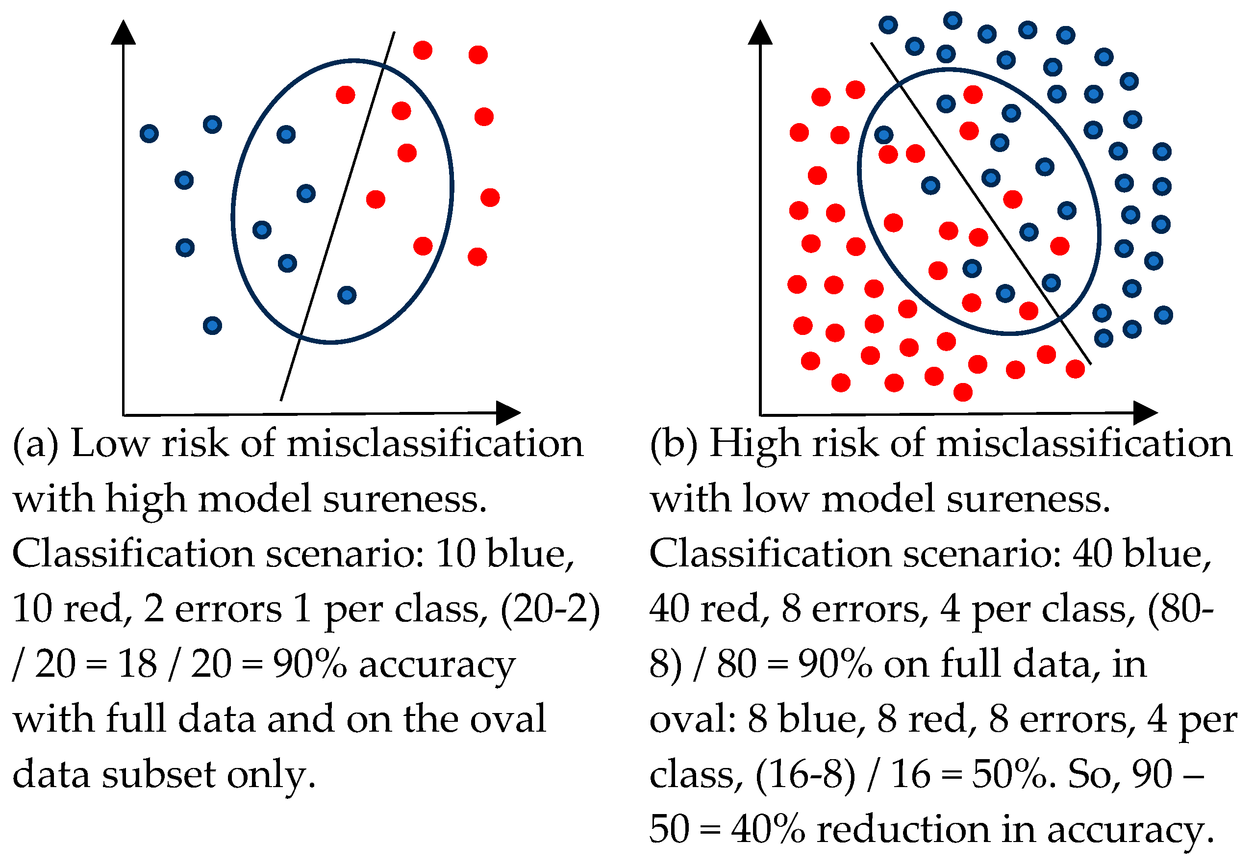
Figure 2.
Examples of different model sureness showing how the addition of one case takes us from an easy classification scenario to a difficult one.
Figure 2.
Examples of different model sureness showing how the addition of one case takes us from an easy classification scenario to a difficult one.
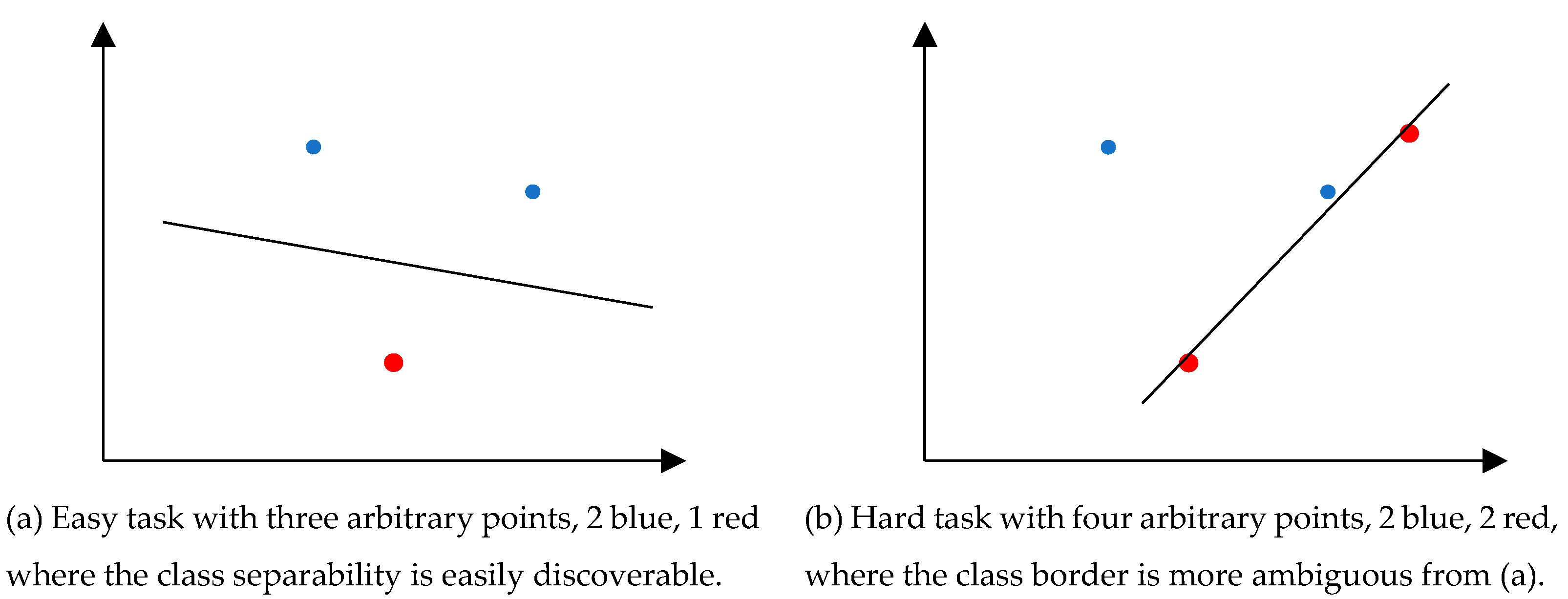
Figure 3.
Diagram of the overall process conducted where we repeat the Update Train Data step iteratively.
Figure 3.
Diagram of the overall process conducted where we repeat the Update Train Data step iteratively.
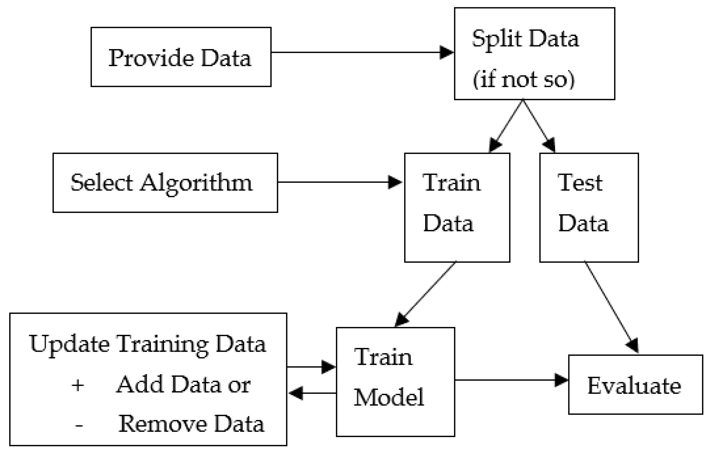
Figure 5.
Visualization of the resultant 9,600 cases from the first MNIST experiment in this study.
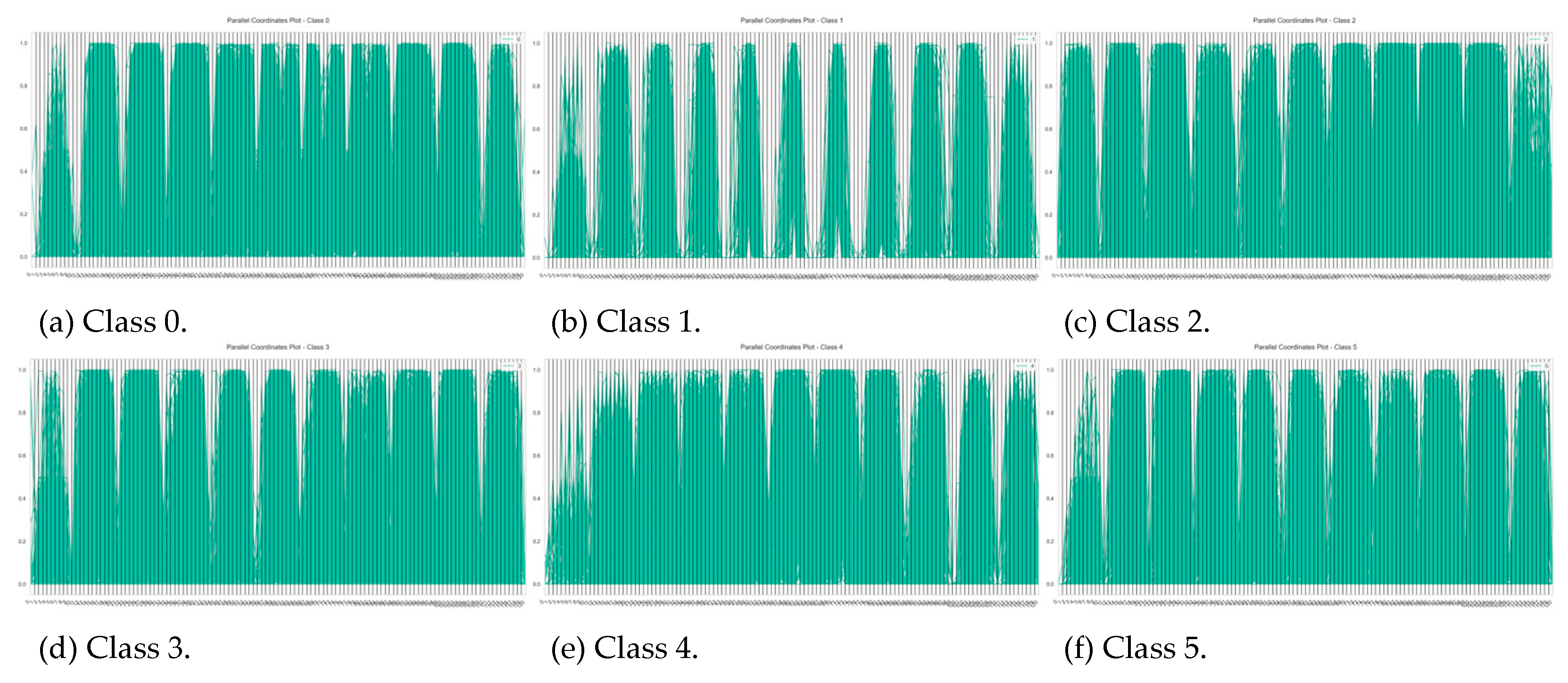
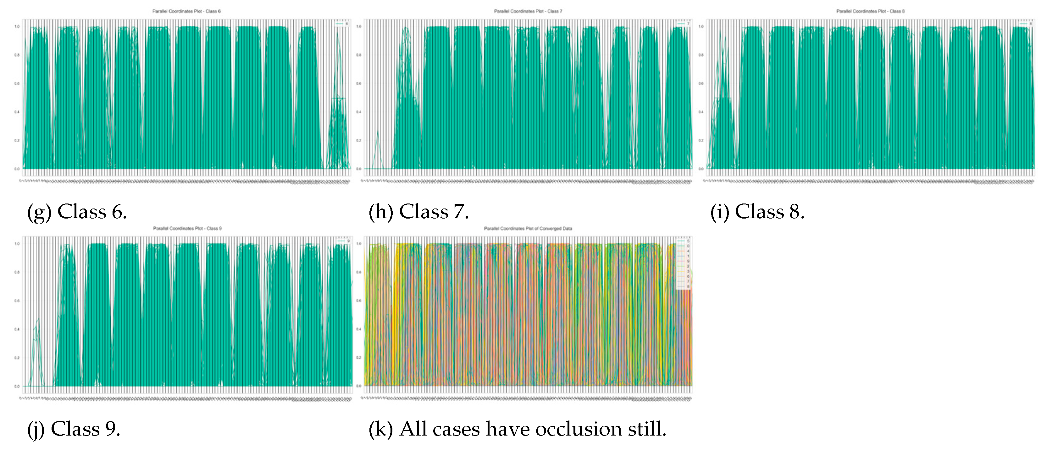
Figure 6.
Visualization of the full 60,000 cases in top two plots, and the reduced stable 9600 cases in the bottom two.
Figure 6.
Visualization of the full 60,000 cases in top two plots, and the reduced stable 9600 cases in the bottom two.
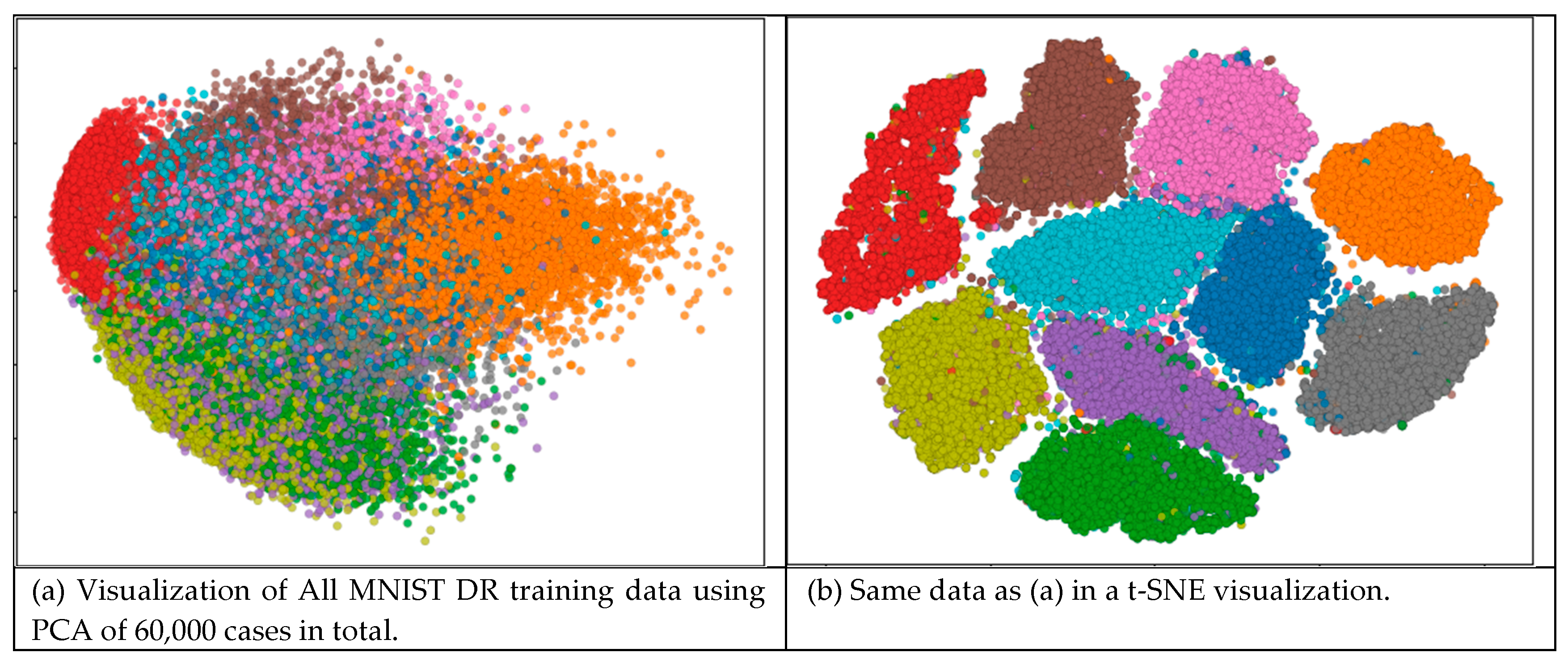
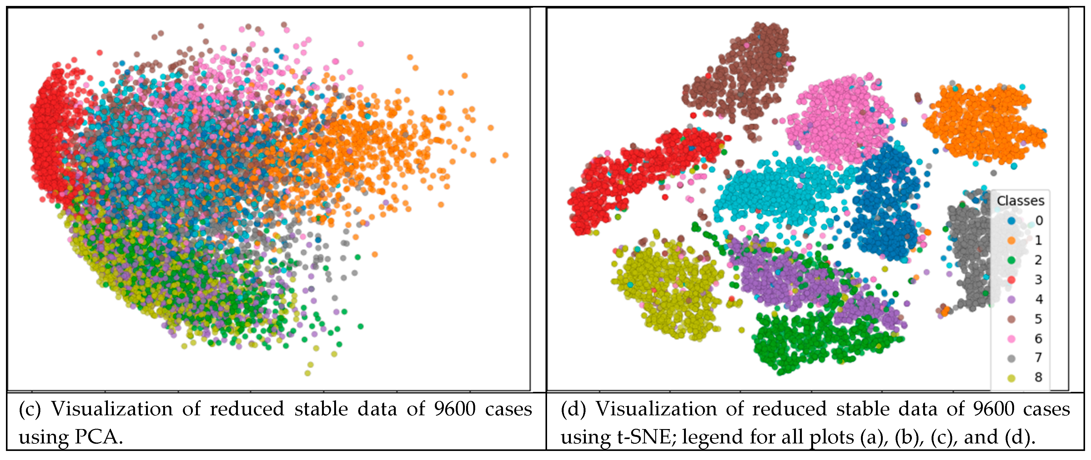
Figure 7.
Visualization of the centroids from the full data on top two plots, and the reduced in bottom two.
Figure 7.
Visualization of the centroids from the full data on top two plots, and the reduced in bottom two.
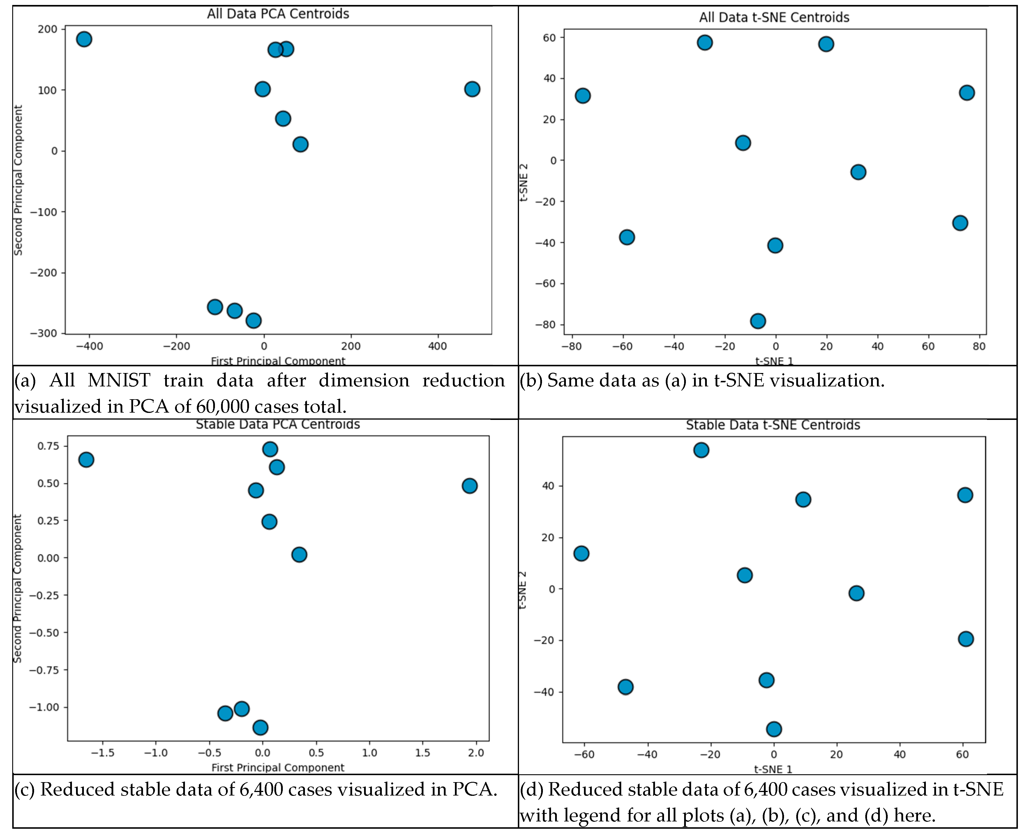
Figure 8.
Results of plotting the top accuracy tests found 2,800 cases in Parallel Coordinates.
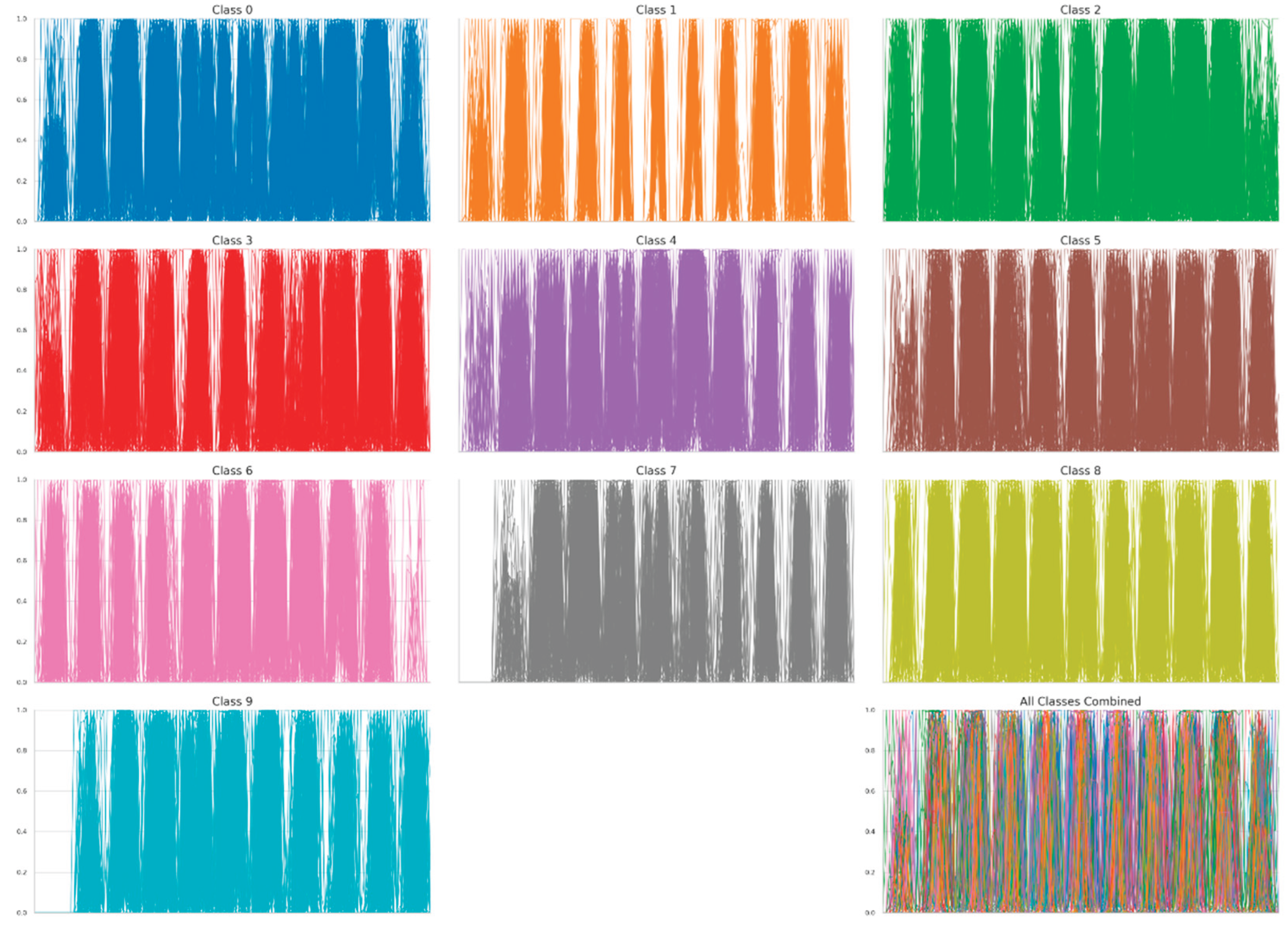
Table 1.
SVM on Fisher Iris data with 10 cases increment, 70:30 split and threshold 95%.
| Characteristics | Number of iterations of SVM run | ||
| 10 | 100 | 1,000 | |
| Mean Cases Needed | 37.8 ± 22 | 31.6 ± 16.5 | 31.8 ± 18.5 |
| Min Cases Needed | 10 | 10 | 10 |
| Max Cases Needed | 90 | 90 | 100 |
| Mean Model Accuracy | 0.953 ± 0.035 | 0.959 ± 0.026 | 0.961 ± 0.026 |
| Convergence Rate* | 9 / 10 = 90% | 93 / 100 = 93% | 919 / 1000 = 91.9% |
*The Convergence Rate is measured by the ratio of the number of times the model was considered as “sure” (under given accuracy threshold) relative to the total number of iterations ran.
Table 2.
Results on Fisher Iris testing LDA data adding 10 cases from 70:30 split to threshold of 95%.
Table 2.
Results on Fisher Iris testing LDA data adding 10 cases from 70:30 split to threshold of 95%.
| Characteristics | Number of iterations of LDA run | ||
| 10 | 100 | 1,000 | |
| Mean Cases Needed | 19 ± 5.4 | 21.3 ± 14.3 | 21.1 ± 14.5 |
| Min Cases Needed | 10 | 10 | 10 |
| Max Cases Needed | 30 | 100 | 100 |
| Mean Model Accuracy | 0.980 ± 0.018 | 0.977 ± 0.021 | 0.977 ± 0.02 |
| Convergence Rate | 10/10 = 100% | 99/100 = 99% | 981/1,000 = 98.1% |
Table 3.
Results of testing Iris HBs have grown with IMHyper algorithm.
| Iteration | Cases in Training data | Hyperblock Count |
Average Hyperblock Size |
Next Misclassified |
| 1 | 5 | 2 | 2.5 | N/A |
| 2 | 5 | 2 | 2.5 | 0/5 |
| 3 | 10 | 2 | 5 | 0/5 |
| 4 | 15 | 2 | 7.5 | 0/5 |
| 5 | 20 | 2 | 10 | 0/5 |
| 6 | 25 | 2 | 12.5 | 0/5 |
| 7 | 30 | 2 | 15 | 0/5 |
| 8 | 35 | 2 | 17.5 | 0/5 |
| 9 | 40 | 2 | 20 | 0/5 |
| 10 | 45 | 2 | 22.5 | 0/5 |
| 11 | 50 | 2 | 25 | 0/5 |
| 12 | 55 | 2 | 27.5 | 0/5 |
| 13 | 60 | 2 | 30 | 0/5 |
| 14 | 65 | 2 | 32.5 | 0/5 |
| 15 | 70 | 2 | 35 | 0/5 |
| 16 | 75 | 2 | 37.5 | 0/5 |
| 17 | 80 | 2 | 40 | 0/5 |
| 18 | 85 | 2 | 42.5 | 0/5 |
| 19 | 90 | 2 | 45 | 0/5 |
| 20 | 95 | 2 | 47.5 | 0/5 |
| 21 | 100 | 2 | 50 | 0/5 |
Table 5.
Test results on MNIST data, with variant test cases up to a total of 60,000 train cases, using 10,000 test cases for each model measurement.
Table 5.
Test results on MNIST data, with variant test cases up to a total of 60,000 train cases, using 10,000 test cases for each model measurement.
| Number of iterations of SVM run | ||
| Characteristics | 10 | 100 |
| Mean Cases Needed | 9,600 | 9,600 |
| Min Cases Needed | 9,600 | 9,600 |
| Max Cases Needed | 9,600 | 9,600 |
| Mean Model Accuracy | 0.972 | 0.972 |
| Convergence Rate | 10/10 = 10% | 100/100 = 100% |
Table 6.
Minimal MNIST training dataset for k-NN with k = 3.
| Cases Per Class Label | Case Count | Percentage |
| 0 | 954 | 9.94% |
| 1 | 1,088 | 11.33% |
| 2 | 946 | 9.85% |
| 3 | 985 | 10.26% |
| 4 | 953 | 9.93% |
| 5 | 834 | 8.69% |
| 6 | 976 | 10.17% |
| 7 | 1,029 | 10.72% |
| 8 | 899 | 9.36% |
| 9 | 936 | 9.75% |
Table 7.
CNN accuracy on all MNIST data. .
| Training Data (all 60,000 training MNIST cases) | Accuracy on all Test Data (10,000 cases) |
| Data 28x28 ( full resolution) | 99.57% |
| Data 11x11 (121-D data by 3 pixels crop edges and average pooling of 2x2 kernel, 2 stride) | 99.34% |
Table 8.
Results of model accuracy given various reduced training data subsets.
| Accuracy on all test data | Sample Count |
| 95.36% | 2,800 |
| 96.25% | 3,200 |
| 95.20% | 2,500 |
| 95.93% | 2,700 |
| 96.79% | 2,800 |
Disclaimer/Publisher’s Note: The statements, opinions and data contained in all publications are solely those of the individual author(s) and contributor(s) and not of MDPI and/or the editor(s). MDPI and/or the editor(s) disclaim responsibility for any injury to people or property resulting from any ideas, methods, instructions or products referred to in the content. |
© 2025 by the authors. Licensee MDPI, Basel, Switzerland. This article is an open access article distributed under the terms and conditions of the Creative Commons Attribution (CC BY) license (http://creativecommons.org/licenses/by/4.0/).
Copyright: This open access article is published under a Creative Commons CC BY 4.0 license, which permit the free download, distribution, and reuse, provided that the author and preprint are cited in any reuse.


