
Submitted:
04 July 2025
Posted:
07 July 2025
You are already at the latest version
Abstract
Supercritical fluid extraction (SFE) using carbon dioxide (CO2) has been extensively investigated in the literature due to its efficiency and environmental compatibility. A key objective of such modeling efforts is the scale-up of laboratory results to pilot or industrial-scale systems. Among the established models, Sovová’s Broken and Intact Cell (BIC) model classifies extraction behavior into four distinct types of extraction curves, corresponding to varying levels of CO2 accessibility during the initial, fast extraction phase from easy to very difficult penetration. Most experimental extractions are categorized as Type A and Type B. However, empirical observations often reveal that extraction behavior during the initial phase deviates from the linear trend predicted by Sovová’s original model. Instead, a nonlinear, decreasing trend is commonly observed.This study focuses on a proposed mathematical model, which uses a power law function of the form e = axb to describe the fast extraction phase. It is then coupled with partial differential equation (PDE) and ordinary differential equation (ODE) to model the slow extraction phase. The proposed model synthesizes key elements from both Sovová’s BIC model and the Reverchon model, replicating Sovová’s approach in the fast extraction phase and aligning with Reverchon’s formulation in the slow extraction phase.The proposed model is demonstrated through experiments involving the supercritical CO2 extraction of argan kernel oil under varying pressures (300–400 bar) and temperatures (40–60 °C). The two non-constant parameters a and b of the power law equation were determined using response surface methodology (RSM) based on the experimental data. These parameters were then used to develop a predictive equation correlating the power law parameters with two pressures and three temperatures, enhancing the model’s predictive accuracy for Type A and B extractions. This proposed mathematical modeling provides a more accurate representation of the extraction kinetics and can serve as a foundation for further extension to other BIC types, thereby extending its use to a wide range of plant matrices in supercritical fluid extraction processes.
Keywords:
BIC model
; argan kernel oil
; supercritical fluid CO2 extraction
; mathematical model
MSC: 76-04
1. Introduction
Supercritical fluid extraction (SFE) using carbon dioxide (CO2) has been extensively applied to a wide variety of plant materials, including seeds, leaves, and kernels. This technique is particularly valued for its ability to extract highly purified essential oils and bioactive compounds, making it especially suitable for applications in pharmaceuticals and nutraceuticals [1,2,3,4,5]. Accurate modeling of the extraction process is crucial for predicting extraction yields and enabling effective scale-up from laboratory to pilot and industrial scale operations. Among the most widely used models for SFE are the Sovová model and the Reverchon model. The Sovová model is derived from mass balance and mass transfer principles. It typically represents the extraction process using exponential functions, segmented into two or three stages depending on the type of extraction curve (Types A–D) [6,7,8]. In contrast, the Reverchon model also originates from mass balance and mass transfer equations but employs partial differential equation (PDE) and ordinary differential equation (ODE) to describe the extraction kinetics, solved using time-dependent numerical methods [9].
In two-dimensional (2D) simulations of supercritical fluid extraction (SFE), partial differential equation (PDE) and ordinary differential equation (ODE) are used to model the entire extraction process [10]. The results in high prediction errors in the initial stages of extraction. This rapid extraction behavior deviates markedly from that of normal extraction processes. In normal extraction processes, the extraction rate shows a decreasing curve during the initial phase, reflecting a rapid decline in mass transfer as easily accessible solutes are depleted. In contrast, supercritical fluid extraction (SFE) often shows a nearly linear extraction curve in the early stage, indicating an efficient extraction rate due to the superior solvating power and high diffusivity of supercritical CO2. However, a significant modeling is required during the initial phase of extraction, where supercritical CO2 rapidly dissolves the target compounds. To solve this issue, several studies have modeled the fast extraction zone using a linear relationship, expressed as e = qys, where e is the extraction oil and “ys” represents solubility [11,12]. In this context, solubility is determined experimentally and is often correlated with temperature and pressure using the Chrastil model [13,14]. While this linear approximation offers simplicity, it does not represent the nonlinear behavior observed during the fast extraction phase of many plant materials.
The primary objective of this study is to develop a unified mathematical model that integrates both the Sovová and Reverchon approaches. The proposed mathematical model divides the extraction process into two phases, consistent with BIC model: a fast extraction phase and a slow extraction phase. The fast extraction phase is characterized using a power law function of the form e = axb, while the slow extraction phase is described using PDE and ODE formulations, following the conceptual basis of the Reverchon model [15]. The simulation is implemented in a one-dimensional (1D) domain. A power law equation of the form e = axb is proposed to describe the kinetics of the fast extraction phase. Unlike linear models, the power law formulation more accurately represents the fast phase, providing improved predictive accuracy and a better fit to experimental data. This approach reflects the rapid mass transfer mechanisms characteristic of supercritical CO2 extraction during the initial phase.
For plant materials with soft outer structures, such as leaves or seeds, the fast extraction phase is commonly approximated by a linear equation, where the extraction rate remains relatively constant. In such cases, solubility defined as a function of pressure and temperature is used directly as the slope in the linear model [16,17,18]. However, it is not suitable for hard-shelled plant materials, such as argan kernels, where the extraction behavior non-linearity due to increased mass transfer resistance. A power law equation is used to represent the fast extraction zone in the proposed model, with its parameters expressed as functions of pressure and temperature. It provides a more accurate representation of such systems. This model is particularly well-suited for Type B extraction behavior in the Sovová BIC. Moreover, the structural similarities between argan kernel, coconut, and palm kernel all of which possess hard shells suggest that this model can be effectively extended to these materials [19,20,21]. The improved predictive capability of the power law-based approach makes it a promising tool for modeling supercritical CO2 extraction in hard-shelled plant matrices.
2. Modeling and Methods
2.1. Mathematical and Numerical Modeling
The fast extraction zone, often referred to as the solubility-controlled region in previous studies, is commonly described using a linear equation of the form e = qys, where the parameter “ys” represents the solubility of the material in supercritical CO2 extraction. This solubility is determined by fitting the linear model to experimental extraction data from the beginning of the process up to a defined critical time (tc), which marks the transition to the slow extraction phase.
In the present study, the fast extraction zone is instead modeled using a power law equation, e = axb, to better represent the non-linear behavior of the extraction process during this phase. The two non-constant parameters “a” and “b” were obtained by fitting the model to experimental data using MATLAB. This approach provides a more accurate representation of the initial phase extraction kinetics.
where e is the extraction oil at fast extraction zone (g), a and b are the non-constant parameters for power law equation, x is amount of CO2 (g).
where is mass flow rate of CO2 (g/min), t is extraction time (min).
e = axb
Once the supercritical CO2 extraction process reaches the critical time (tc), the extraction rate begins to decline significantly, which indicates the transition from the fast extraction zone to the slow extraction zone as shown in Figure 1. In this later phase, mass transfer becomes limited by internal diffusion within the solid matrix. To accurately describe the extraction behavior in the slow extraction zone, partial differential equation (PDE) and ordinary differential equation (ODE) were used. For more detailed please see [10,22].
PDE
ODE
where is porosity, V is volume of extractor (m3), c is oil concentration in fluid phase (g), u is superficial velocity (m/s), Ap is total particle area (m2), K is mass transfer coefficient (m/s), is oil concentraction in solid phase (g), is oil concentraction at interface (g).
Both equations can be solved using numerical methods in the COMSOL program. The initial conditions are set at the critical time (tc), with the initial oil concentration defined as
Initial time derivative:
where RoE is rate of extraction (g/min), is determined by the slope at the critical time (tc) point within the fast extraction zone.
In this study, the yield of oil concentration was expressed in dimensionless units to allow comparison with the experimental data from the Argan study [23]. The calculation is performed using the following equation:
2.2. Initial and Boundary Condition
The proposed model consists of two phases: the fast extraction zone and the slow extraction zone. The fast extraction zone is described using a power law equation (Eq. (1) & Eq. (2)).
Initial conditions: For t = 0
e(0) = 0
x(0) = 0
The PDE and ODE was solved by numerical method using the backward Euler method. The numerical simulations are conducted in a one-dimensional (1D) domain using COMSOL Multiphysics. The mesh was defined as a line representing the height of the extraction column along vertical axis. Following the governing equations (Eq. (3) and Eq. (4)).
Initial conditions: For t = tc
c(tc) = 0
Boundary conditions: For h = 0
c(0) = 0
Assume tc is defined as the final point within the experimental data that corresponds to the end of the fast extraction zone and the onset of the slow extraction zone. If multiple data points are recorded within the range surrounding tc, the estimation of this transition point becomes more accurate. is initial oil concentration in solid phase (g).
2.3. Validation
In previous studies, the fast extraction zone has commonly been described using a linear equation, where solubility was used as the parameter, representing a constant rate of extraction under supercritical conditions [11,13]. In contrast, the present study begins by investigating the actual extraction behavior within the fast extraction zone and proposes a power law equation (Eq. (1)) as a more appropriate model to describe the observed nonlinearity.
To validate this approach, experimental data from the supercritical CO2 extraction of argan kernel oil were used. The predicted extraction curves, combining the power law equation for the fast extraction zone and PDE/ODE-based modeling for the slow extraction zone, were compared against the experimental results. Within the fast extraction zone, data points prior to the critical time (tc) were fitted to the power law equation to obtain the two non-constant parameters, “a” and “b”. These parameters were determined for all experimental conditions across various temperatures and pressures, with the resulting values presented in Table 1.
Following the determination of non-constant parameters “a” and “b” from the power law fitting, the RSM equation was developed to relate these parameters to the operating conditions specifically pressure and temperature. An RSM fitting approach was used to model the dependence of each parameter on pressure and temperature (Eq. (7)). The use of the RSM equation to calculate the two non-constant parameters enables the model to make predictions without the need for experimental data at specific pressure and temperature conditions. This significantly enhances the model’s predictive capability and practical applicability. In this model, the pressure and temperature are treated as the independent variables along the X and Y axes, respectively, while the resulting non-constant parameter value (either “a” or “b”) forms the Z-axis.
The general form of RSM equation used is
where Z is the power law parameter i.e. a or b. X and Y are dimensionless pressure and temperature, respectively. X = [0,1] and Y = [-1,0,1].
Z = p0 + p1X + p2Y + p12XY + p22Y2
MATLAB was used to perform curve fitting and determine the parameters of the RSM equations for predicting the non-constant parameters “a” and “b” in the power law model. These equations allow for the estimation of the power law parameters as functions of pressure and temperature, enabling prediction of extraction yield in the fast extraction zone under varying operating conditions. The parameter of the RSM equations presented in Table 2.
In the slow extraction zone, the extraction behavior is controlled by internal diffusion. This slow phase is modeled using a system of coupled partial differential equation (PDE) and ordinary differential equation (ODE) (Eq. (3) & Eq. (4)). These equations were solved by numerical method using the Backward Euler method, implemented in the COMSOL Multiphysics. The simulation is designed to ensure continuity between the fast and slow extraction phases. The slope at tc (RoEtc) was used to calculate the parameter ApK, which represents the apparent efficiency of oil extraction (Eq. (5)). Once the ApK parameter is determined, the PDE and ODE can be solved, allowing for the accurate simulation of the slow extraction phase. This enhancing the overall accuracy of the hybrid model.
A reverse validation was conducted using the predicted two non-constant parameters “a” and “b” obtained from the RSM equations as functions of pressure and temperature (Eq. (7)). The non-constant parameters “a” and “b” are plotted as surface curves, with pressure and temperature as the x and y-axes, respectively, as shown in Figure 2. These predicted parameters were substituted into the power law equation to simulate the extraction yield in the fast extraction zone. The resulting predicted curves using the RSM-based model (Eq. (7)) were then compared against both the experimental data and the fitted curves derived directly from experimental “a” and “b” values. The results from the power law and PDE/ODE models were converted to oil yield using Eq. (6). The Root Mean Square Error (RMSE) were used to assess the goodness of fit in each case.
3. Results and Discussion
3.1. Comparison Between Experimental Fitting and Modeling with RSM
The experimental data and model extraction curve are presented in Figure 3. The solid lines represent curves obtained by fitting the experimental data, while the dashed lines represent the model curves based on the parameters from Eq. (7). The extraction curves fitted from experimental data showed low error. Similarly, the model-generated curves based on parameters derived from Eq. (7) also showed small errors, though slightly higher than those from direct experimental curve fitting. The non-constant parameters in Eq. (7) were obtained using MATLAB by fitting experimental data across various pressure and temperature conditions. This equation provides a reliable means of predicting the non-constant parameters “a” and “b” in the power law model and is therefore appropriate for simulating extraction yields under different operating conditions.
An interesting observation was made at 40 °C, where the extraction rate at 300 bar was higher in the initial phase than at 400 bar. This behavior deviates from typical supercritical extraction trends, where an increase in pressure usually corresponds to a higher initial yield. This phenomenon is attributed to the retrograde solubility effect, a well-known anomaly in supercritical fluid extraction. Retrograde behavior refers to the inverse relationship between pressure and solubility at lower temperatures, where increasing pressure leads to a decrease in extraction efficiency during the initial phase, as shown in Figure 3 (a).
As shown in Figure 2, the parameter “a” decreases at lower temperatures. Under such conditions, the density of the supercritical CO2 becomes less influential, and diffusion limitations dominate the mass transfer process. At high pressure, the viscosity of the fluid increases, which in turn reduces diffusion rates, as described by the Stokes–Einstein equation. As a result, oil molecules require more time to move from within the solid matrix to the surface, delaying the onset of efficient extraction. Despite this complexity, the model based on Eq. (7) continues to show strong agreement with experimental data, affirming its suitability for modeling supercritical CO2 extraction.
3.2. Slow Extraction Zone and Fast Extraction Zone
In the fast extraction zone, the data are modeled using the power law equation (Eq. (1)), as the actual extraction behavior shows nonlinearity and cannot be accurately represented by a simple linear model. The use of the power law function shows the rapid yet nonlinear extraction that occurs during this phase, as shown in Figure 4. The non-constant parameters “a” and “b” in the power law equation are closely related to the solubility of the target compounds in supercritical CO2. These parameters vary as functions of pressure and temperature (Figure 2), which significantly influence solute solubility and mass transfer rates in the extraction process. The critical time (tc) is defined as the time corresponding to the final experimental data point before the transition from the fast to the slow extraction zone. This transition point is crucial for accurately connecting the power law model with the PDE/ODE-based model used for the slow extraction phase.
The non-constant parameters “a” and “b” from the power law equation e = axb exhibit clear trends with respect to extraction conditions. The parameter “a”, which represents the initial slope of the extraction curve, increases with temperature, meaning enhanced solubility and mass transfer at higher thermal conditions. In contrast, the parameter “b”, which controls the rate of curvature or declines in the extraction profile, increases with pressure. Both non-constant parameters remain less than 1 (Table 1), indicating a decreasing extraction rate over time, consistent with the observed non-linear behavior during the fast extraction phase. The parameter “a” is explained as the initial rate of mass transfer. At the beginning of the extraction (typically within the range of CO2 consumption below approximately 5 kg CO2/kg material), this phenomenon shows a shell extraction behavior. The parameter “b”, which defines the degree of curvature in the power law model, accords the rate of decrease in extraction over time. At lower pressures, “b” values are smaller, leading to a sharper decline in the extraction rate. Conversely, as pressure increases, “b” approaches 1, causing the curve to become more linear. A value of b≈1 signifies a relatively constant extraction rate, which is characteristic of Type A extraction kinetics typical for soft plant matrices such as leaves or seeds with permeable outer layers. Under these conditions, both the experimentally fitted curves and the curves predicted by the RSM model (Eq. (7)) show good agreement, confirming the validity of the model for predicting the fast extraction phase.
After the critical time (tc), the extraction process transitions into the slow extraction zone, where the extraction behavior is described by a system of partial differential equation (PDE) and ordinary differential equation (ODE). This phase begins with a slope equal to that at tc, ensuring continuity between the fast and slow extraction models. The slope at this point is used to determine the value of ApK, a parameter representing the apparent extraction efficiency (Eq. (5)). The ApK value is calculated based on the final yield and slope of the power law curve at tc. The PDE and ODE are derived from mass balance and mass transfer principles. As the extraction time progresses, the mass transfer rate slowly decreases due to the decreasing concentration of extractable oil within the particles, as shown in Figure 4. This modeling approach describes the extraction process across both zones and ensures that the overall extraction curve is smooth and accurate.
3.3. Comparison Between BIC Type B Model and Proposed Model
In A. Mouahid study on argan extraction [23], the fast extraction zone was subdivided into two phases: the initial phase was modeled using a solubility based linear equation, followed by a second phase described by another linear equation. As a result, the Sovová BIC model for Type B extraction typically uses two separate equations to characterize the fast extraction zone. The dashed lines in Figure 5, these models based on linear and exponential equations are advantageous due to their simplicity and ease of implementation, and they provide acceptable predictive accuracy for Type B systems.
In contrast the solid lines of Figure 5, the present study introduces an improved approach by representing the entire fast extraction zone using a single power law equation. This not only simplifies the model but also improves predictive accuracy. Importantly, the proposed model requires fewer experimental parameters than the original BIC model. Specifically, only three parameters need to be estimated: the non-constant parameters “a” and “b” from the power law equation, and the transition time tc to the slow extraction phase. Beyond this point, the slow extraction zone is described using PDE and ODE formulations, which are solved numerically via the Backward Euler method.
The effectiveness of the proposed model is showed by its strong agreement with experimental data and lower prediction error compared to the BIC Sovová model, as shown in the comparison in Figure 5. As summarized in Eq. (1)-(4) and detailed in Table 3, the model provides a complete and accurate for predicting extraction yield across different operational conditions. These results confirm the model’s reduced complexity, and superior accuracy in modeling supercritical CO2 extraction.
3.4. Error of Modeling and Experimental
As shown in Table 4, the error associated with the Sovová BIC model is generally less than 2%, which is considered acceptable for predictive modeling in supercritical fluid extraction. However, to further enhance the accuracy of yield prediction and reduce the residual error, the proposed model developed in this study combining a power law equation for the fast extraction zone with PDE/ODE formulations for the slow extraction zone demonstrates superior performance. The error between the experimental data and the curve obtained from MATLAB fitting using the power law model was found to be less than 1% for most operating conditions, demonstrating excellent agreement, as shown in Table 4. The only exception was observed at 400 bar and 50 °C, where a slightly higher deviation was recorded, likely due to experimental variability or nonlinear effects not fully captured at that specific condition.
Additionally, the model predicted curve generated using the non-constant parameters “a” and “b” obtained from the RSM equations based on pressure and temperature also showed a comparable level of accuracy to that of the experimentally fitted model. This indicates that the predictive model for solubility-based parameters is reliable and effective in simulating the extraction yield in the fast extraction zone across a range of conditions.
4. Conclusions
In previous studies on the modeling of supercritical fluid extraction (SFE), the fast extraction zone has often been represented using a linear equation, assuming a constant extraction rate. For greater accuracy, the extraction behavior in the fast extraction zone is modeled with a slightly decreasing rate. In this study, the extraction behavior in the fast extraction zone is more accurately described using a power law equation (Eq. (1) & Eq. (2)), which accounts for the slight decrease in extraction rate over time. The non-constant parameters “a” and “b” in the power law model are both less than 1, as shown in Table 1, decreasing nature of the extraction curve. When b=1, the model simplifies to a linear form, corresponding to Type A extraction behavior, which is typical of soft plant materials such as leaves or seeds with permeable outer shells. In contrast, when b<1, the model indicates a Type B extraction behavior, characterized by a declining extraction rate in the early stages. This behavior is commonly observed in hard-shelled materials such as argan kernel, coconut, palm kernel, and similar plant matrices. The power law model thus provides a more flexible and realistic for describing SFE kinetics, particularly for materials with structural barriers to concentration release in the early extraction phase.
Pressure and temperature directly influence the solubility of the oil concentration in supercritical CO2 and are modeled using a response surface methodology (RSM) equation, as shown in Figure 2. To determine the non-constant parameters “a” and “b” of the power law equation, experimental extraction data are used to fit the extraction curves in the fast extraction zone. Subsequently, RSM equations correlating these parameters to pressure and temperature are developed (Eq. (7)). This approach effectively links the power law model to operating conditions, enabling accurate description of extraction behavior in the fast extraction phase.
The transition between the fast and slow extraction zones occurs at the critical time tc, which is estimated from experimental data. Beyond tc, the extraction kinetics are controlled by coupled PDE and ODE models that describe the decreasing extraction rate characteristic of the slow extraction zone. The combined model shows strong agreement with the Sovová Broken and Intact Cells (BIC) model for Type B extraction behavior, as shown in Figure 4. The RMSE of this model is less than 1% due to the improved equation, indicating higher accuracy compared to previous studies, as shown in Figure 5. This mathematical model effectively describes the extraction process and accurately predicts the yield across all extraction conditions.
Supplementary Materials
The following supporting information can be downloaded at: https://www.mdpi.com/article/doi/s1.
Author Contributions
Methodology, T.O. and W.L.; Software, T.O.; Formal analysis, T.O. and W.L.; Writing—original draft, T.O. and W.L.; Writing—review & editing, T.O. and W.L.; Supervision, W.L. All authors have read and agreed to the published version of the manuscript.
Funding
This research received no external funding.
Data Availability Statement
The original contributions presented in this study are included in the article/Supplementary Materials. Further inquiries can be directed to the corresponding author.
Acknowledgments
This study was supported by Thammasat University Research Fund, Contact No TUFT 100/2567 and Thammasat University Center of Excellence in Computational Mechanics and Medical Engineering, Thammasat University, Pathum Thani, Thailand.
Conflicts of Interest
The authors declare no conflicts of interest. The funders had no role in the design of the study; in the collection, analyses, or interpretation of data; in the writing of the manuscript; or in the decision to publish the results.
Abbreviations
| SFE | Supercritical fluid extraction |
| BIC | Broken and intact cell |
| PDE | Partial differential equation |
| ODE | Ordinary differential equation |
| RoE | Rate of extraction |
| RSM | Response surface methodology |
References
- Park, H.; Kim, J.S.; Kim, S.; et al. Pharmaceutical applications of supercritical fluid extraction of emulsions for micro-/nanoparticle formation. Pharmaceutics 2021, 13(11), 1928. https://doi.org/10.3390/pharmaceutics13111928. [CrossRef]
- Artemiev, A.I.; Demkin, K.M.; Kazeev, I.V. Search for New Active Substances for the Development of Pharmaceuticals Using Supercritical Fluid Extraction. Biochemistry (Moscow) Supplement Series B: Biomedical Chemistry 2024, 18(4), 323–330. https://doi.org/10.1134/S1990750824600511. [CrossRef]
- Oman, M.; Škerget, M.; Knez, Z. Application of supercritical fluid extraction for the separation of nutraceuticals and other phytochemicals from plant material. Macedonian Journal of Chemistry and Chemical Engineering 2013, 32(2), 183–226. https://doi.org/10.20450/mjcce.2013.443. [CrossRef]
- Li, L.; Chen, M.; Zeng, Y.; Liu, G. Application and Perspectives of Supercritical Fluid Technology in the Nutraceutical Industry. Advanced Sustainable Systems 2022, 6(7), 2200055. https://doi.org/10.1002/adsu.202200055. [CrossRef]
- Khalil, A.A.; Rahman, M.M.; Rauf, A.; et al. Oleuropein: Chemistry, extraction techniques and nutraceutical perspectives-An update. Critical Reviews in Food Science and Nutrition 2024, 64(27), 9933–9954. https://doi.org/10.1080/10408398.2023.2218495. [CrossRef]
- Sovová, H.; Rate of the vegetable oil extraction with supercritical CO2-I modeling of extraction curves. Chem. Eng. Sci. 1994, 49 (3), 409–414. https://doi.org/10.1016/0009-2509(94)87012-8. [CrossRef]
- Sovova, H.; Kucera, J.; Jez, J. Rate of the vegetable oil extraction with supercritical CO2–II extraction of grape oil. Chem. Eng. Sci. 1994, 49(3), 415–420. https://doi.org/10.1016/0009-2509(94)87013-6. [CrossRef]
- Mouahid, A.; Claeys-Bruno, M.; Clercq, S. A New Methodology Based on Experimental Design and Sovová’s Broken and Intact Cells Model for the Prediction of Supercritical CO2 Extraction Kinetics. Processes 2024, 12(9), 1865. http://doi.org/10.3390/pr12091865. [CrossRef]
- Reverchon, E. Mathematical modeling of supercritical extraction of sage oil. AIChE J. 1996, 42(6), 1765–1771. https://doi.org/10.1002/aic.690420627. [CrossRef]
- Obchoei, T.; Limtrakarn, W. Axisymmetric flow model of cannabis oil extraction of supercritical fluid extraction CO2 process. International Journal of Thermofluids. 2024, 22, 100682. https://doi.org/10.1016/j.ijft.2024.100682. [CrossRef]
- Mouahid, A.; R´ebufa b, C.; Le Dr´eau, Y. Supercritical CO2 extraction of Walnut (Juglans regia L.) oil: Extraction kinetics and solubility determination. Journal of Supercritical Fluids. 2024, 211, 106313. https://doi.org/10.1016/j.supflu.2024.106313. [CrossRef]
- Zuknik, M.H.; Nik Norulaini, N.A.; Wan Nursyazreen Dalila, W.S.; et al. Solubility of virgin coconut oil in supercritical carbon dioxide. Journal of Food Engineering. 2016, 168, 240–244. http://dx.doi.org/10.1016/j.jfoodeng.2015.08.004. [CrossRef]
- Del Vallea, J.M.; De la Fuente, J.C.; Uquichec, E. A refined equation for predicting the solubility of vegetable oils in high pressure CO2. Journal of Supercritical Fluids. 2012, 67, 60– 70. https://doi.org/10.1016/j.supflu.2012.02.004. [CrossRef]
- Tomita, K.; Machmudah, S.; Quitain, A.T.; et al. Extraction and solubility evaluation of functional seed oil in supercritical carbon dioxide. J. Supercrit. Fluids. 2013, 79, 109–113. https://doi.org/10.1016/j.supflu.2013.02.011. [CrossRef]
- Reverchon, E.; Donsi, G.; Osseo, L.S. Modeling of supercritical fluid extraction from herbaceous matrices. Ind. Eng. Chem. Res. 1996, 32(11), 2721–2726. https://doi.org/10.1021/ie00023a039. [CrossRef]
- Hartono, R.; Mansoori, G. A.; Suwono, A. Prediction of solubility of biomolecules in supercritical solvents. Chemical Engineering Science. 2001, 56(24), 6949–6958. https://doi.org/10.1016/s0009-2509(01)00327-x. [CrossRef]
- Vatani, Z.; Ramezanian Bajgiran, S.; Amini, G. Solubility modeling of supercritical fluid extraction in a wide range compounds: comparison between fuzzy-genetic and new empirical models. Energy Sources Part A: Recovery Utilization and Environmental Effects. 2020, 42(3), 365–374. https://doi.org/10.1080/15567036.2019.1587083. [CrossRef]
- Sodeifian, G.; Usefi, M.M.B. Solubility, Extraction, and Nanoparticles Production in Supercritical Carbon Dioxide: A Mini-Review. ChemBioEng Reviews. 2023, 10(2), 133–166. https://doi.org/10.1002/cben.202200020. [CrossRef]
- Torres-Ramóna, E.; García-Rodríguezb, C.M.; Estévez-Sánchezc, K.H.; et al. Optimization of a coconut oil extraction process with supercritical CO2 considering economical and thermal variables. Journal of Supercritical Fluids. 2021, 170, 105160. https://doi.org/10.1016/j.supflu.2020.105160. [CrossRef]
- Promraksaa, A.; Siripatanaa, C.; Rakmaka, N.; et al. Modeling of Supercritical CO2Extraction of Palm Oil and TocopherolsBased on Volumetric Axial Dispersion. Journal of Supercritical Fluids. 2020, 166, 105021. https://doi.org/10.1016/j.supflu.2020.105021. [CrossRef]
- Zaidul, I.S.M.; Nik Norulaini, N.A.; Mohd Omar, A.K.; et al. Supercritical carbon dioxide (SC-CO2) extraction of palm kernel oil from palm kernel. Journal of Food Engineering. 2007, 79, 1007–1014. https://doi.org/10.1016/j.jfoodeng.2006.03.021. [CrossRef]
- Obchoei, T.; Limtrakarn, W.; Numerical model of supercritical fluid extraction CO2 technique for cannabis extraction. Eur. Chem. Bull. 2023, 12(6), 7354–7364. https://doi.org/10.31838/ecb/2023.12.si6.654. [CrossRef]
- Mouahid, A.; Bombarda, I.; Claeys-Bruno, M.; et al. Supercritical CO2 extraction of Moroccan argan (Argania spinosa L.) oil: Extraction kinetics and solubility determination. Journal of CO2 Utilization. 2021, 46, 101458. https://doi.org/10.1016/j.jcou.2021.101458. [CrossRef]
Figure 1.
Fast and slow extraction zone on supercritical CO2 extraction process.
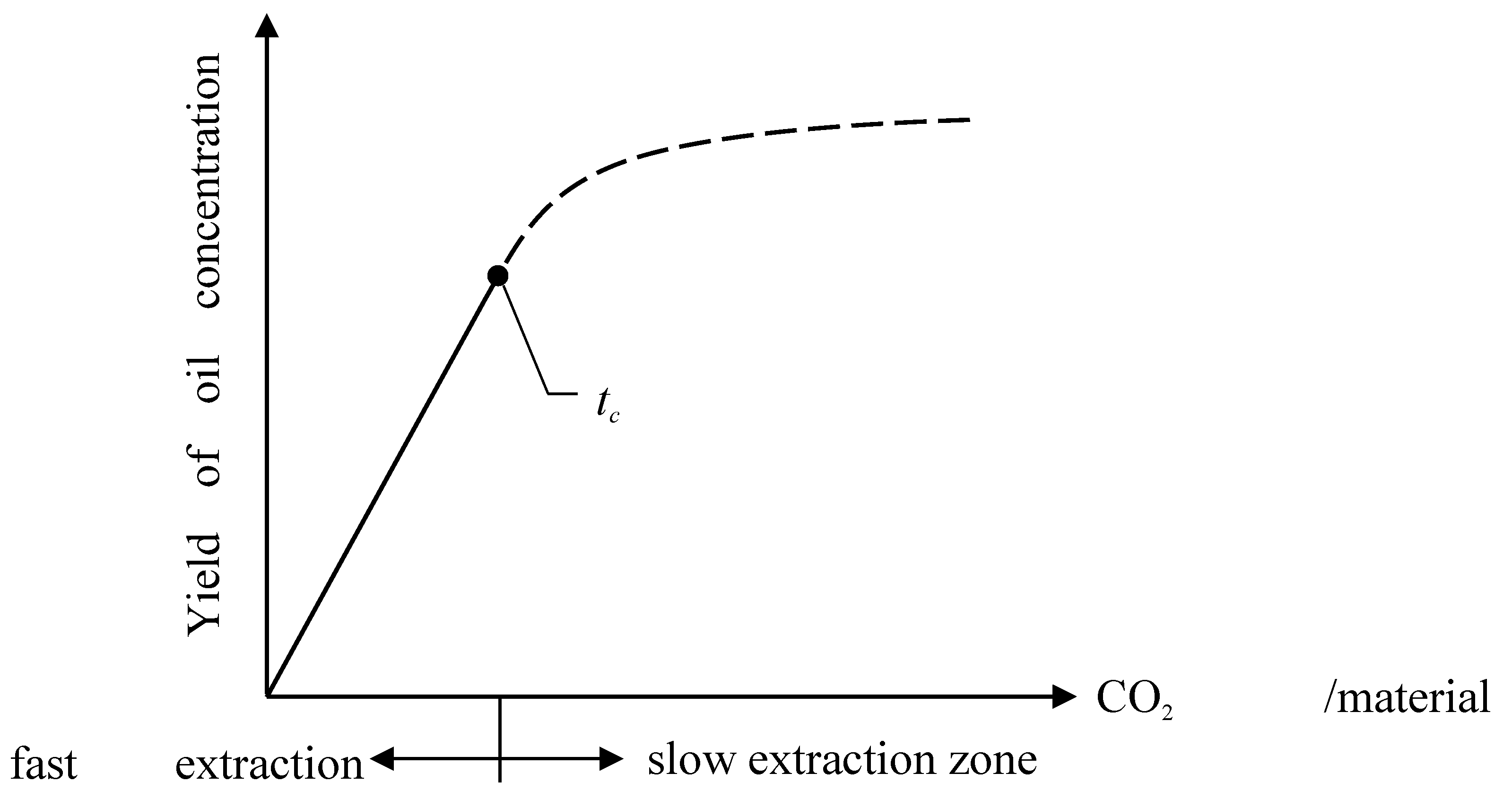
Figure 2.
RSM chart for non-constant parameters “a” and “b” varies with temperature and pressure. (a.) Parameter “a”, (b.) Parameter “b”.
Figure 2.
RSM chart for non-constant parameters “a” and “b” varies with temperature and pressure. (a.) Parameter “a”, (b.) Parameter “b”.
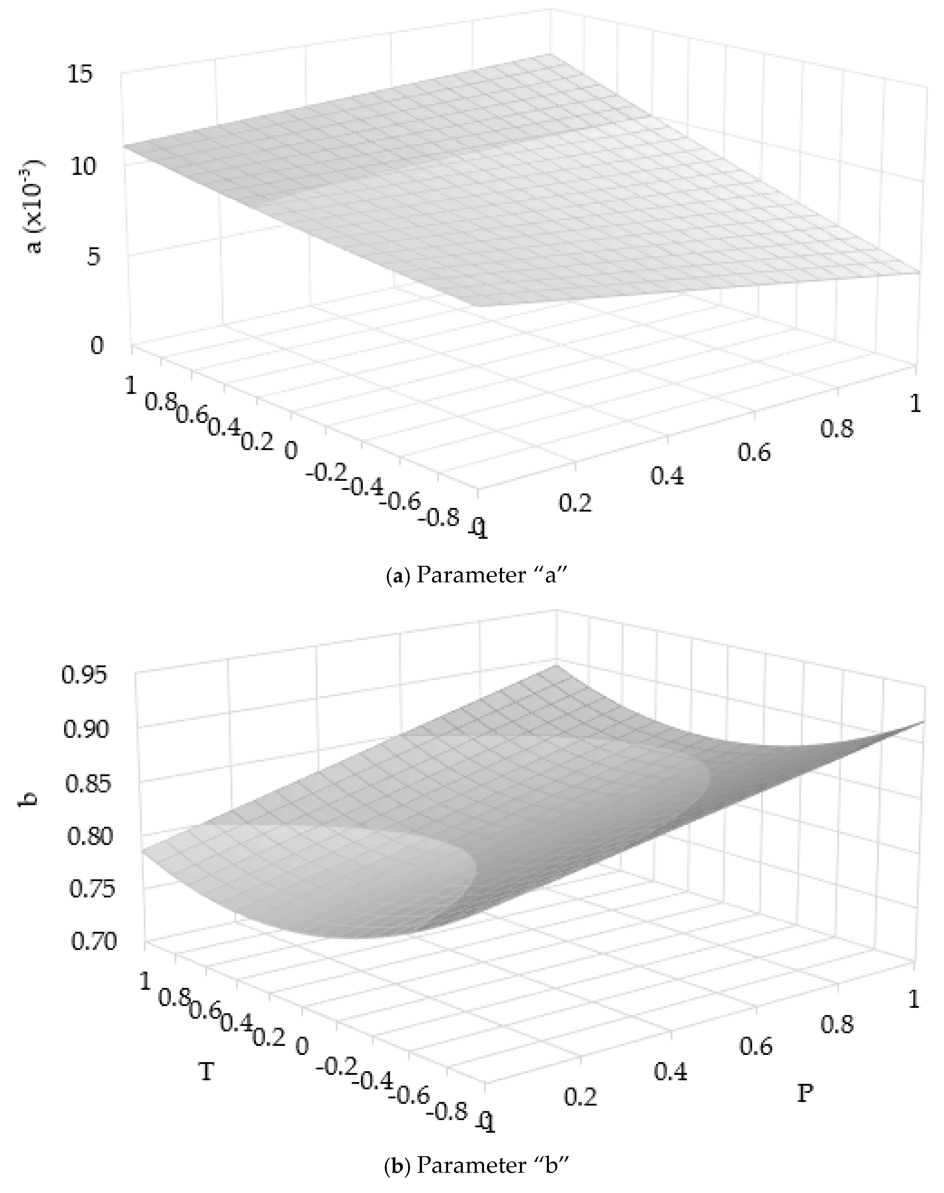
Figure 3.
Yield of oil concentration by amount of CO2 in dimensionless unit. Show experimental fitting and modeling combine with Eq. (7). (a.) 40 °C, (b.) 50 °C, (c.) 60 °C.
Figure 3.
Yield of oil concentration by amount of CO2 in dimensionless unit. Show experimental fitting and modeling combine with Eq. (7). (a.) 40 °C, (b.) 50 °C, (c.) 60 °C.
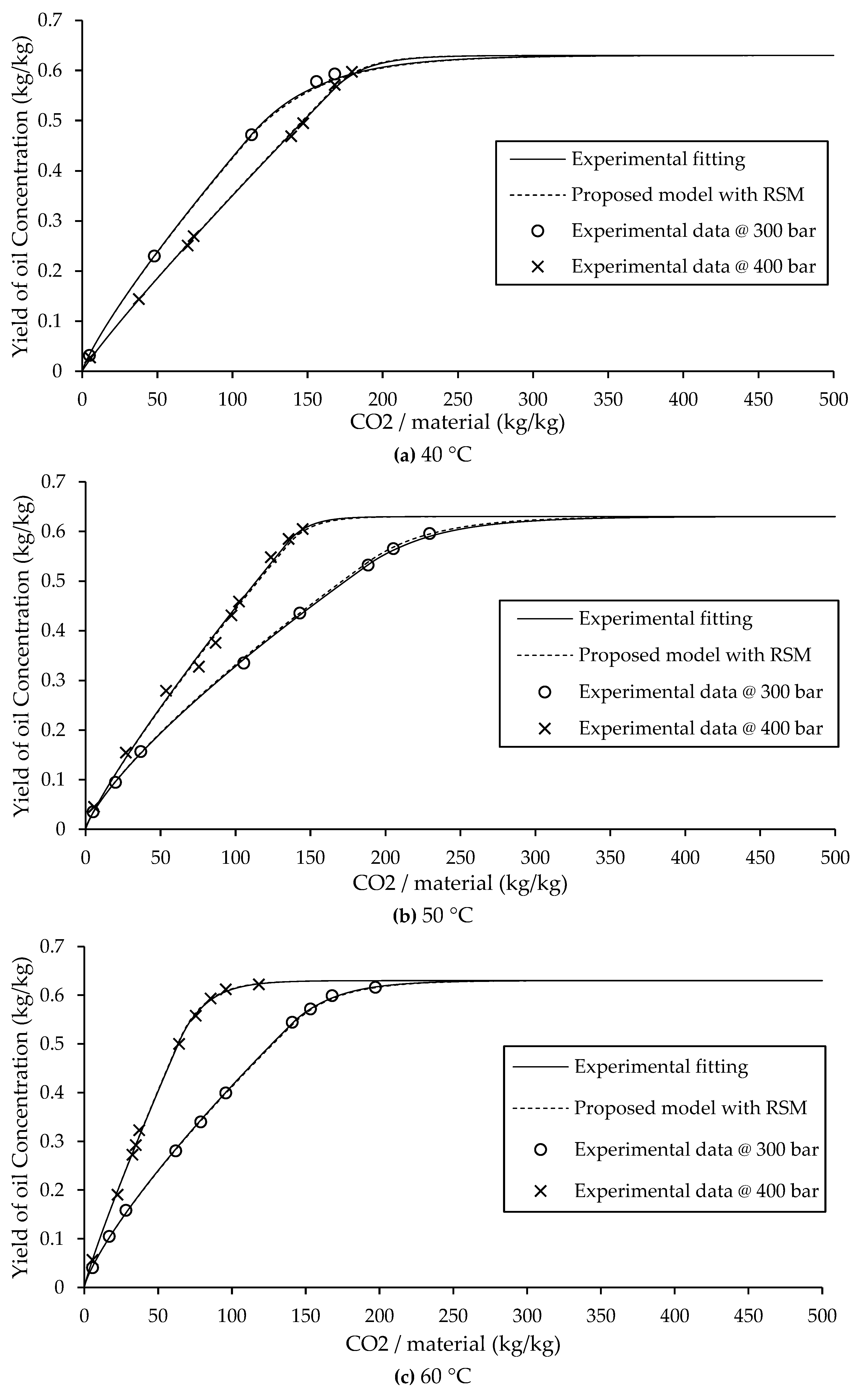
Figure 4.
Yield of oil concentration by amount of CO2 in dimensionless unit. Show fast extraction zone and slow extraction zone. (a.) 40 °C, (b.) 50 °C, (c.) 60 °C.
Figure 4.
Yield of oil concentration by amount of CO2 in dimensionless unit. Show fast extraction zone and slow extraction zone. (a.) 40 °C, (b.) 50 °C, (c.) 60 °C.
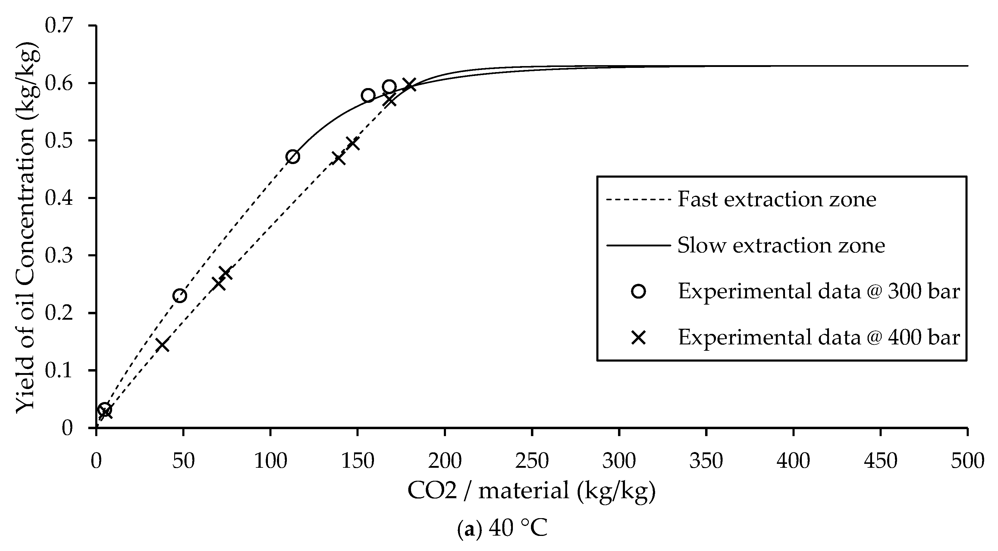
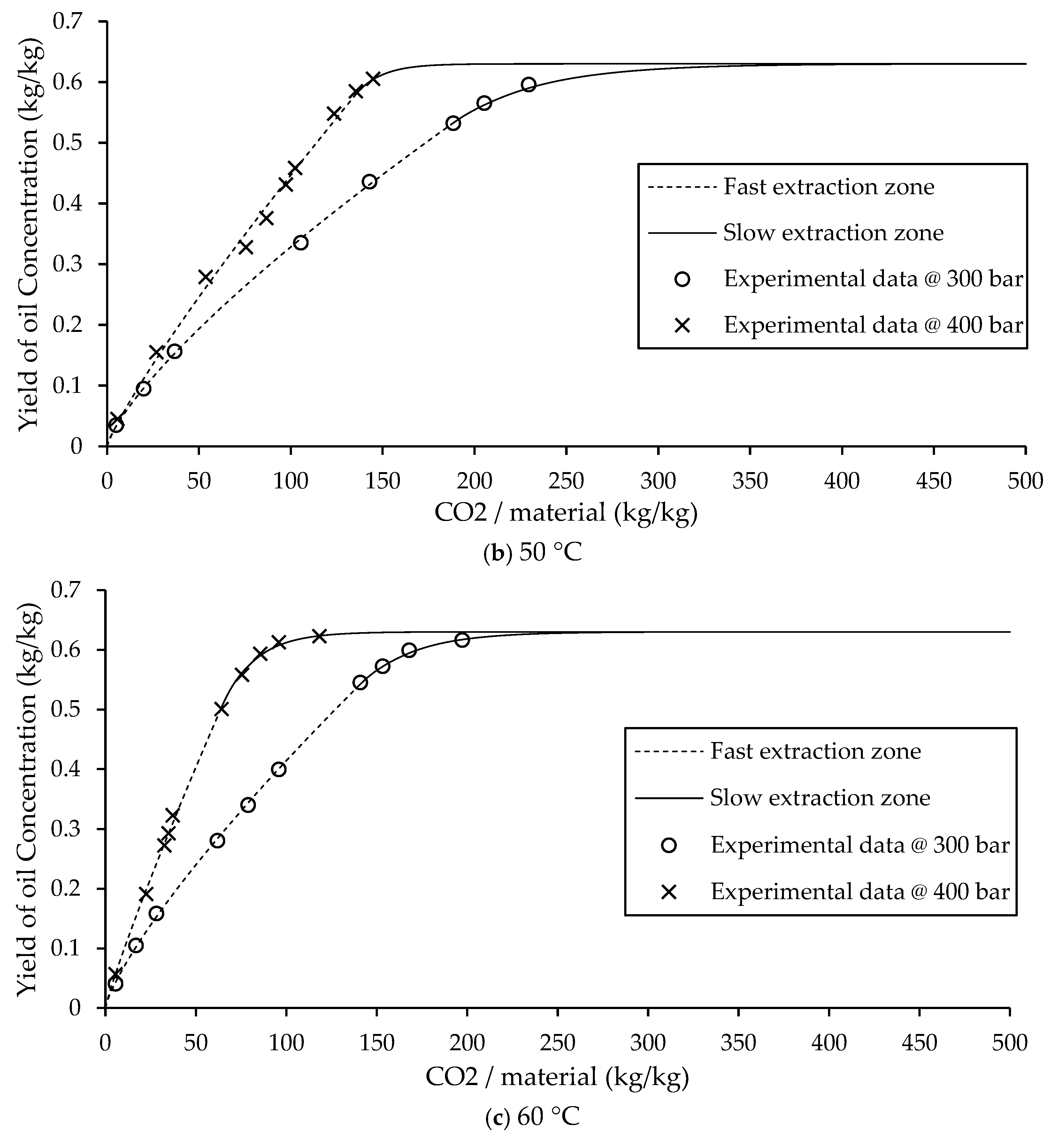
Figure 5.
Yield of oil concentration by amount of CO2 in dimensionless unit. Show proposed model and BIC model. (a.) 40 °C, (b.) 50 °C, (c.) 60 °C.
Figure 5.
Yield of oil concentration by amount of CO2 in dimensionless unit. Show proposed model and BIC model. (a.) 40 °C, (b.) 50 °C, (c.) 60 °C.
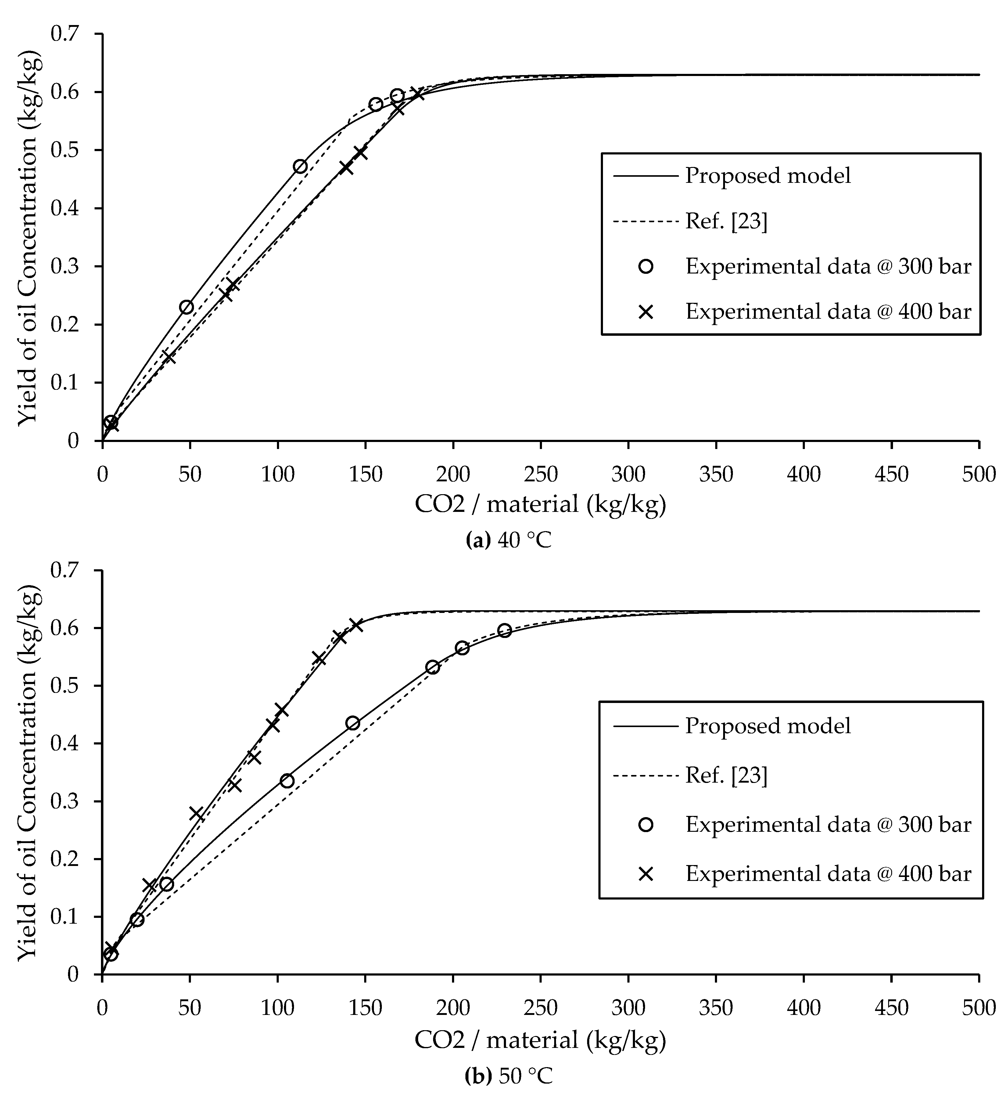
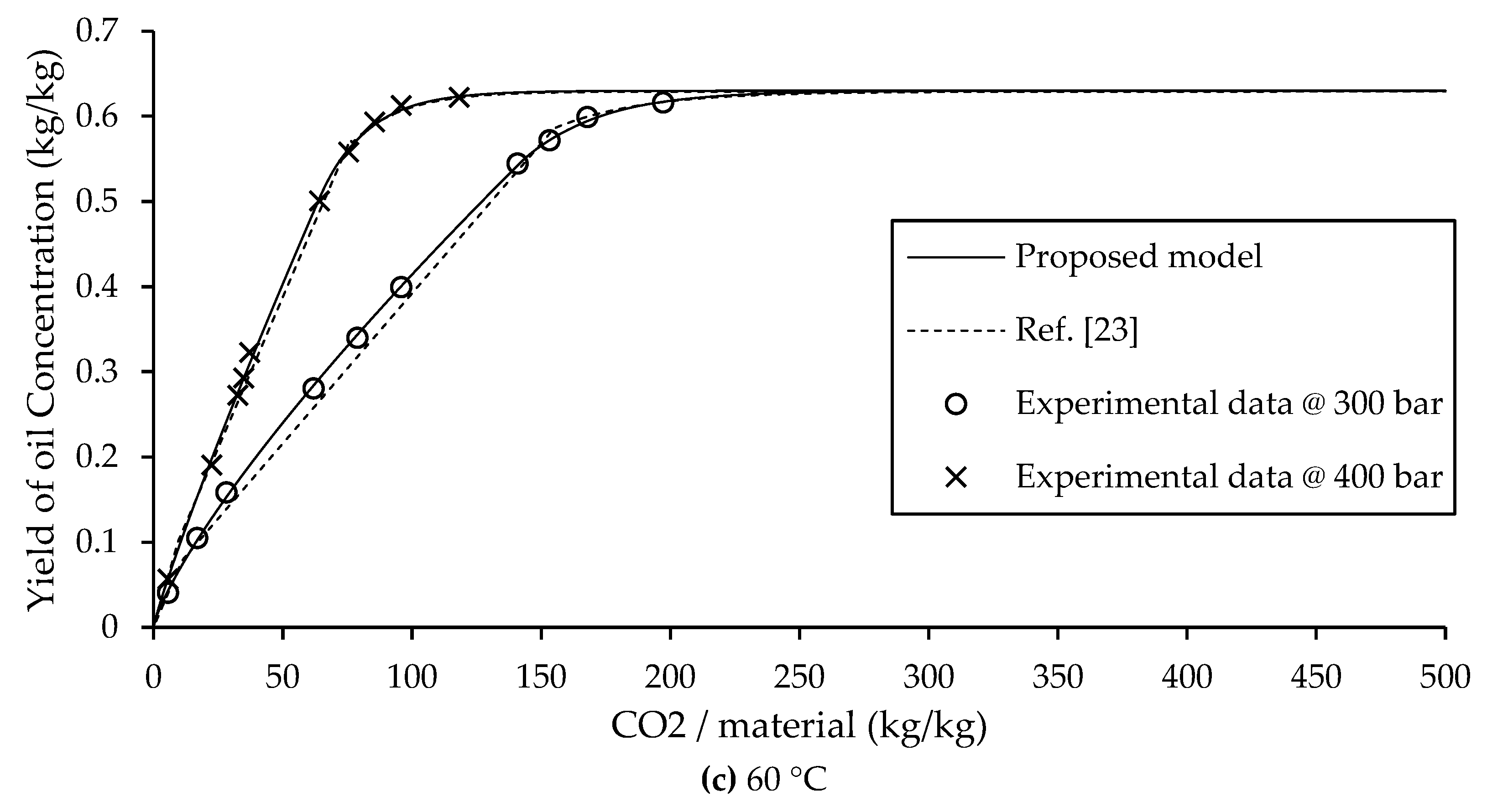

Table 1.
Parameters “a” and “b” are used in power law equation.
| Temperature | Pressure | a | b |
| 40 | 300 | 0.008808 | 0.8427 |
| 400 | 0.00511 | 0.918 | |
| 50 | 300 | 0.00978 | 0.7631 |
| 400 | 0.008491 | 0.8605 | |
| 60 | 300 | 0.01103 | 0.7872 |
| 400 | 0.01229 | 0.8921 |
Table 2.
Parameters of RSM equation for “a” and “b”.
| Coefficient | a | b |
| p0 | 0.009757 | 0.7655 |
| p1 | -0.001242 | 0.09253 |
| p2 | 0.001111 | -0.02775 |
| p12 | 0.002479 | 0.0148 |
| p22 | 0.000174 | 0.0482 |
Table 3.
Equation for predict yield.
| Authors | Equation of Fast extraction zone | Equation of Slow extraction zone |
| A. Mouahid [23] |
e = qys for q < q1 e = q1ys+(q-q1)Kxt for q1 < q < qc |
e = xu[1-C1exp(-C2q)] for q > qc |
| This study | e = a(t)b for t < tc | for t > tc |
Table 4.
Error of 1D simulation.
| Temperature (°C) | Pressure (bar) | Model fit from experimental data (RMSE) |
Model fit from RSM equation (RMSE) |
BIC model (RMSE) |
| 40 | 300 | 0.68% | 0.82% | 1.86% |
| 400 | 0.44% | 0.45% | 0.56% | |
| 50 | 300 | 0.96% | 1.05% | 3.24% |
| 400 | 1.26% | 1.31% | 1.30% | |
| 60 | 300 | 0.32% | 0.37% | 1.44% |
| 400 | 0.55% | 0.56% | 1.09% |
Disclaimer/Publisher’s Note: The statements, opinions and data contained in all publications are solely those of the individual author(s) and contributor(s) and not of MDPI and/or the editor(s). MDPI and/or the editor(s) disclaim responsibility for any injury to people or property resulting from any ideas, methods, instructions or products referred to in the content. |
© 2025 by the authors. Licensee MDPI, Basel, Switzerland. This article is an open access article distributed under the terms and conditions of the Creative Commons Attribution (CC BY) license (http://creativecommons.org/licenses/by/4.0/).
Copyright: This open access article is published under a Creative Commons CC BY 4.0 license, which permit the free download, distribution, and reuse, provided that the author and preprint are cited in any reuse.


