Submitted:
05 July 2025
Posted:
07 July 2025
You are already at the latest version
Abstract
Mobile charging robots (MCRs), essentially high-voltage batteries mounted on mobile platforms, offer a flexible solution for electric vehicle (EV) charging, particularly in environments like supermarket parking lots with photovoltaic (PV) generation. Unlike fixed charging stations, MCRs must be strategically dispatched and recharged to maximize operational efficiency and revenue. This study investigates a Model Predictive Control (MPC) approach using Mixed-Integer Linear Programming (MILP) to coordinate MCR charging and movement, accounting for the additional complexity that EVs can park at arbitrary locations. The performance impact of EV arrival and demand forecasts is evaluated, comparing perfect foresight with data-driven predictions using Long Short-Term Memory (LSTM) networks. A slack variable method is also introduced to ensure timely recharging of the MCRs. Results show that incorporating forecasts significantly improves performance compared to no prediction, with perfect forecasts outperforming LSTM-based ones due to better-timed recharging decisions. The study highlights that inaccurate forecasts—especially in the evening—can lead to suboptimal MCR utilization and reduced profitability. These findings demonstrate that combining MPC with predictive models enhances MCR-based EV charging strategies and underlines the importance of accurate forecasting for future smart charging systems.
Keywords:
Smart Charging
; Electric Vehicles
; Mobile Charging Robot
; DC Charging
; Model Predictive Control
; Long Short-Term Memory Network
; Energy Management
1. Introduction
In order to meet the climate goals set by the Paris Agreement and to reduce greenhouse gas emissions, a transformation of the mobility and transport sector is essential. The increasing importance of E-mobility is already evident [1]. A major challenge associated with E-mobility is the development and management of charging infrastructure. While users demand charging solutions that are convenient, reliable, and fast, charge point operators (CPOs) prioritize return-on-investment (ROI), and grid operators must ensure grid stability.
The growing adoption of electric vehicles (EVs) has also highlighted the significance of public charging infrastructure. According to the International Energy Agency [2], public charging solutions are expected to play a crucial role in the global EV ecosystem. These solutions complement home and fleet charging options by addressing the needs of EV users in urban and high-traffic areas. Various approaches have been proposed to account for the diverse interests of stakeholders. Smart charging and bi-directional charging strategies are gaining prominence in fleet management and home charging scenarios. In public and semi-public settings, battery storage concepts are increasingly utilized to minimize the need for grid reinforcement while still delivering high charging power and fast charging capabilities. However, a fundamental challenge remains: although stationary battery-supported charging solutions provide flexibility to the grid, they do not offer the same level of flexibility to users. If all charging ports are occupied, users are unable to charge their vehicles immediately or may have to return later.
The deployment of mobile charging robots, such as the GINI robot introduced by Wessel et al. [3], presents several advantages over stationary solutions. These mobile robots enhance flexibility in charging location, potentially improving user satisfaction by reducing wait times and optimizing charging infrastructure utilization. Moreover, they can help balance the load by charging their own batteries during off-peak hours and discharging stored energy during peak demand periods, thereby alleviating grid strain. Nevertheless, mobile charging robots involve higher initial investment and operational costs compared to stationary alternatives. While they have the potential to increase revenue by serving a greater number of vehicles, the financial viability of such systems must be carefully assessed.
Faßbender et al. [4] introduced a simulation environment that models charging infrastructure, grid connections, and user behavior. This environment facilitates the evaluation of MCRs within a public charging context. Built upon the OpenAI Gym framework [5], the simulation environment is modular and extensible, incorporating a rule-based charging controller as a baseline for comparison with advanced charging strategies. In this work, an advanced charging strategy is presented. For this purpose, optimization-based approaches are considered as they are able to provide a systematic and efficient solution to the charging management problem by taking into account the objective and constraints of the system. A short overview of the state-of-the-art in charging management is provided in the following.
A review of optimization-based approaches for EV charging management reveals two predominant methodologies. The first models the system as a stochastic problem, often using constrained Markov Decision Processes (MDPs). Huang et al. [6] decompose the EV charging management problem in a microgrid and solve it via stochastic programming. Huang et al. [7] and Huang et al. [8] apply MDP formulations with dedicated solution methods. Similarly, Fallah-Mehrjardi et al. [9] employs multi-stage stochastic programming, while Yang et al. [10] propose a stochastic MPC based on multi-scenario sampling. Nguyen and Choi [11] introduce a distributionally robust MPC for energy management with V2G and V2V capabilities. These methods often lead to high computational costs, necessitating scenario-based reformulations that require offline pre-computation.
The second predominant approach involves the implementation of deterministic optimization, frequently in conjunction with an MPC approach as presented by Ju et al. [12], Yang et al. [13,14] and D’Amore et al. [15]. The underlying problem is mostly formulated as MILP, if an optimization for individual EVs is desired [12,14]. The MPC approach requires accurate predictions, but only few publications such as [16,17] provide approaches for it. In addition to the initial forecasts, a comprehensive approach requires updates based on the actually observed EV charging demands and connection times.
The aforementioned literature, addresses the charging management problem, but does not consider MCRs. An optimization under consideration of MCRs is presented by Ju et al. [12]. However, the optimization targets a cost analysis and not a real-time controller and hence is not conducted in a receding horizon fashion. Further, the robot considered is mobile in nature, but does not appear to carry a battery storage, which is a key feature of the MCRs considered here.
This work will focus on deterministic optimization and provide the following contributions:
- Adaption of optimization problem for MPC-based charging management with mobile charging robots (MCRs)
- Forecast model based on long short-term memory (LSTM) networks for EV arrivals
- Evaluation of the MPC controller in the simulation environment and comparison of performance with perfect forecast, LSTM based forecast and terminal penalty
2. Materials and Methods
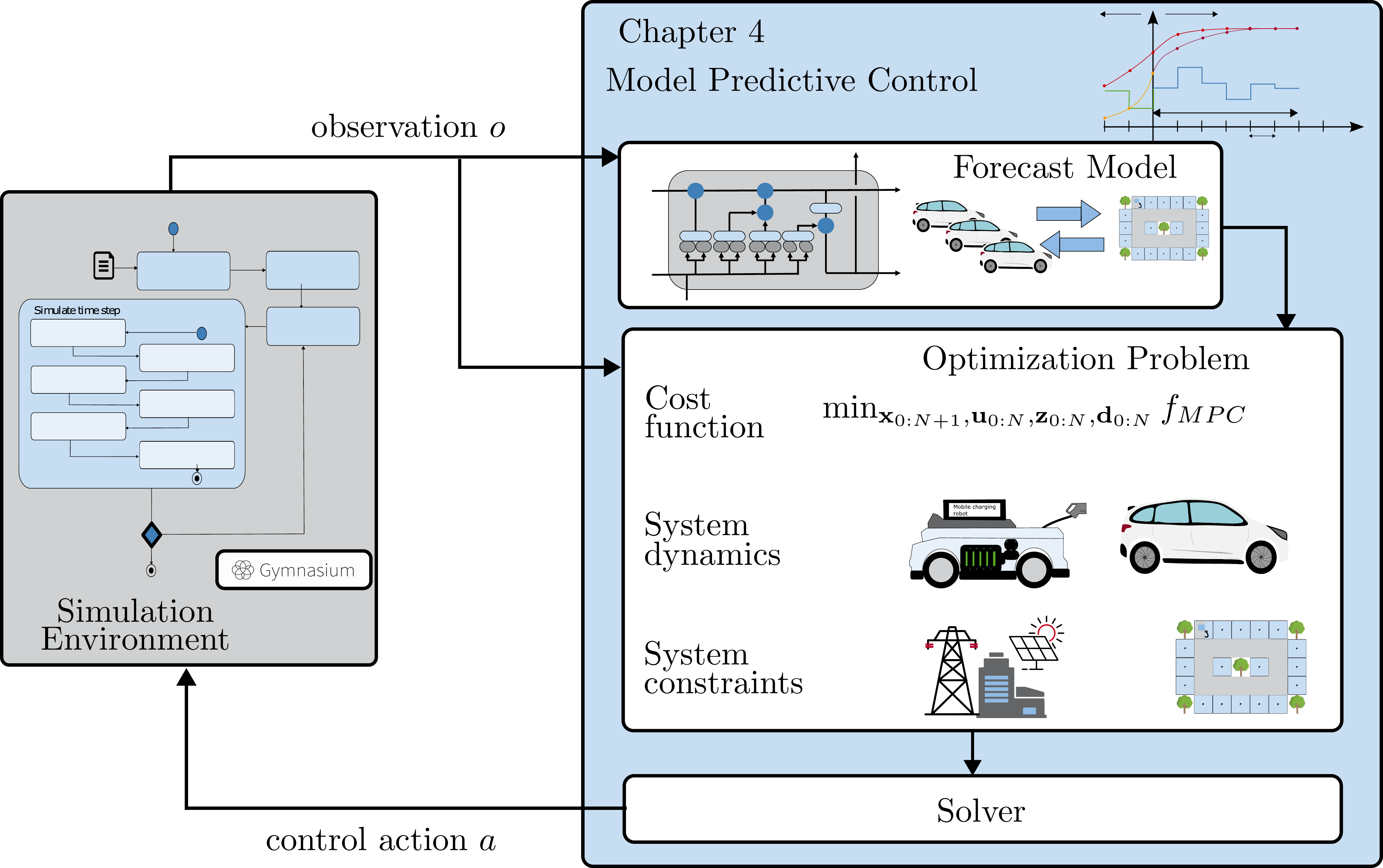
In this section, the methodology is presented. Firstly, the formulation of the mixed-integer linear optimization problem for the MPC controller is introduced. Consecutively, the limitations of the basic formulation, without considering an explicit forecast model, are highlighted. Two approaches are presented, how to deal with the limitations. Firstly, the optimization formulation is extended to provide a motivation to recharge during idling times for the MCRs. Secondly, the forecast model is introduced and the training process elaborated.
All preliminary analysis within this section as well as the comparison within the result section is conducted within the simulation environment presented by Faßbender et al. [4]. The simulation environment considers a parking area and the grid connection point with a building load, photovoltaic and the charging stations. The MCRs are able to recharge at the charging stations. All arriving EVs park at a parking spot and request a MCR for charging. An overview of the key elements of the simulation environment is provided in Figure 1.
The parking area is modeled as a grid of parking fields, where the EVs can park. The MCRs are able to move between the parking fields and the charging station. The power balance is shown in Figure 1 (b). The building load is supplied by the grid and the PV array. The charging stations are connected to the grid and the MCRs are able to charge at them. The MCRs are also able to discharge their stored energy into the grid. The controller (in this case the MPC) can be used to provide set-points for the charging power at the charging stations and for the power with which the MCRs charge an EV. Further the controller can set target fields for the MCRs to move to. In the given setup only MCRs are recharged at CSs and EVs are only recharged by the MCRs. An EV could also be charged directly at the CS. Although, this case is not considered in this work. The configuration used throughout this work can be found in Table 1.
2.1. Optimization Problem for MPC
To formally define the optimization problem, we first introduce the following indices, variables and conventions:
- Prediction horizon index , denoting the discrete step within the prediction horizon . The “absolute” time step index based on the current time would be .
- Mobile Charging Robot (MCR) index , identifying the specific MCR under consideration.
- Charging station index , referring to a specific charging station or charger location.
- Parking field index , indicating the designated parking field under consideration.
- Binary variables: All binary variables are indicated by use of the symbol . indicates the MCR r is located at CS c. The abbreviation “mtc” is used to denote “move to charger”. indicates the MCR r is located at parking field f. The abbreviation “mtp” is used to denote “move to parking field”.
- Sign convention for continuous variables: The continuous variables describing power satisfy .
The OP formulation is implemented using Pyomo [18]. Pyomo is an open source software package for formulating and solving large-scale optimization problems.
The optimization objective is defined through a cost function that may incorporate terminal costs, state-dependent penalties, control effort, and costs associated with continuous control variables. In this specific application, the primary goal is to maximize profit. Consequently, the revenue generated by charging EVs using MCRs is taken into account as described in Eq. 1, where the fixed selling price is multiplied by the total energy delivered by the MCRs. Conversely, the energy procurement cost is based on the time-varying electricity price and the amount of energy obtained from the grid, as shown in Eq. 2. It is assumed that the price profile across the optimization horizon is known in advance. Since the formulation requires a minimization problem, the profit — being the difference between revenue and cost — is represented by multiplying the net cost term by (see Eq. 3).
The cost function is subject to a set of constraints and the system’s dynamic behavior, which will be detailed in the subsequent sections. All constraints presented are enforced at each time step within the prediction horizon, i.e., for every . For readability, the time index will be omitted in the notation unless its inclusion enhances clarity.
As a first constraint, the system must satisfy the power balance at the grid connection point. At each time step , this balance is enforced as defined in Eq. 4. To properly account for the direction of energy flow in the cost formulation, it is necessary to distinguish between the power drawn from the grid and the power fed into the grid . For this purpose, a binary variable and corresponding auxiliary equations are introduced, as shown in Eqs. 5–7.
Simultaneous charging from and feeding power back to the grid is not permitted. A direct modeling of this behavior using the binary variable in Eq. 5 would, however, introduce nonlinearity into the system. To preserve linearity, the big-M formulation is adopted, as proposed in [19]. By incorporating Eq. 6 and Eq. 7 with a sufficiently large constant (set here to ), it is guaranteed that only one of the two auxiliary variables representing grid power flow is active at any time step. This approach ensures that the model remains a mixed-integer linear program.
Each MCR must be located at exactly one field, which can either be a parking spot or a charging spot, as stated in Eq. 8. Furthermore, each field can only be occupied by a single robot at any given time, as enforced by the constraints in Eq. 9 and Eq. 10.
The power capabilities of both the MCRs and the EVs are also bounded and subject to their respective location. Accordingly, the following constraints apply for each MCR r:
If an MCR is connected to a charger, its charging power is constrained by the charger’s maximum capability, as defined in Eq. 11. Additionally, the MCR’s own maximum charging capability imposes a further limit, as given in Eq. 12. When not connected to a charger, the discharging power of the MCR, denoted by , must not exceed its maximum discharging power (see Eq. 13).
Discharging by an MCR is only meaningful if it is co-located with an EV on a parking field. This relationship is modeled using Eq. 14 and Eq. 15. Specifically, Eq. 14 allows the total discharging power to be distributed across all parking locations, while Eq. 15 ensures that discharging occurs exclusively at the location where both the MCR and an EV are present.
Since Eq. 15 introduces a nonlinear relationship, it is relaxed using the Big-M technique. This yields a set of linear constraints, given in Eq. 16–18, which approximate the original condition while preserving the problem’s linear structure.
Power delivery to an EV is only permitted if an EV is currently present or is expected to arrive at a given prediction step . This condition is enforced through Eq. 19.
The change in the energy state of the MCRs is determined by the difference between the charging power and the discharging power , integrated over time, and added to the previous energy state , as described in Eq. 22.
For the EVs, a similar approach is applied, but only the charging power is considered. The energy requirement represents the difference in energy needed at field f to reach the desired state of charge.
As part of the receding horizon optimization approach, at each time step , an observation o is received from the environment. This observation serves as the basis for updating the optimization problem formulation. As indicated in Eq. 23, the energy request for an EV at the current time step k (i.e., ) depends on this state. Additionally, the availability of EVs must also be updated. While the requested energy can be directly obtained from the environment, the availability for the current time step is known. The future availability — and therefore the duration of stay — is estimated based on the average historical stay duration. It is important to note that, in this initial version of the MPC controller, no explicit forecasting is applied. Only the EVs currently present in the parking area are considered in the optimization problem, and no assumptions are made regarding the arrival of new EVs within the prediction horizon.
2.2. Limitations of the Initial Approach
The proposed MPC will be tested over a representative two-day period, from 00:00 on 2nd June 2023 to 24:00 on 3rd June 2023. The results will be analyzed, and strategies for improving and extending the MPC will be derived.
For solving the OP, the Gurobi solver [20] is used. It should be noted that, particularly when dealing with multiple MCRs and longer prediction horizons, solving the problem exactly using the default solver settings is not feasible due to the large problem size and complexity. Consequently, less stringent settings have been applied, as summarized in Appendix A.
The resulting trajectory from applying the MPC controller outlined in section 2.1 to the simulation environment is shown in Figure 2. A prediction horizon of 96 steps, each lasting 5 minutes, was applied.
In the top graph (a), the power balance, including contributions from the charging stations (CSs), the building, and the PV array, is shown. Over the two-day period, 26 recharging events are identified by the spikes in , which also affect the grid power . In the bottom graph (e), the number of EVs present in the parking area is depicted. It can be observed that a maximum of five EVs are present at any given time, with the highest occupancy occurring between 12:00 h and 18:00 h on both days. Notably, EV arrivals are sparse during the nighttime hours. In graph (c), the State of Charge (SoC) of the MCR is shown. Upon the arrival of the first EVs, the MCR discharges down to 20% SoC. Subsequently, the SoC fluctuates between 10% and 50%, reflecting the brief charging and discharging periods. Even during the night, when no EVs arrive for several hours, the SoC remains around 40%. The cost structure, based on accumulated revenue from energy sold and electricity costs , is displayed in plot (b). It is observed that during the first day, temporarily exceeds ; however, after 19:00 h, as EVs are no longer present and building power persists through the night, remains above . The increase in is significantly higher on the first day compared to the second day, primarily due to the starting SoC of 100% and higher, more stable PV power. By the end of the second day, the difference between and results in a profit of €-15.29.
Several aspects of the strategy implemented by the MPC controller are unsatisfactory. The following key observations should be highlighted:
- No recharging without EVs present: In general the MCR only recharges if EVs are present, which is strategically not a good time, because until the MCR is recharged the EVs might have left. Especially during the period between 20:00 h and 04:00 h there are no EVs at the parking area. Therefore, the MCR could recharge. Due to the structure of the optimization problem, where recharging is only attractive if an EV is present to which the charged energy could be sold, this does not happen.
- No “smart” charging: It is observed that, in most cases, the MCR operates at a high power level of approximately 50 kW. However, the charging times do not correspond to periods of low energy costs (refer to plot (d)) or periods of high PV power. It is hypothesized that if charging times and power were to be synchronized with electricity prices and PV power, costs could be reduced.
In summary, the observations suggest that the MPC controller is limited in its ability to anticipate future revenue, primarily due to its inability to account for potential revenue from EVs not currently present at the parking area.
To address these shortcomings, two alternative approaches are proposed. The first approach introduces a penalty for not recharging during idle periods, incentivizing more consistent operation. The second approach incorporates a forecasting model to predict future EV arrivals, utilizing Long Short-Term Memory (LSTM) networks. The training process and integration of this forecasting model into the MPC controller are described in detail.
2.3. Penalty for Not Recharging
One of the main drawbacks identified in the basic MPC approach is its inability to recharge during extended periods of inactivity. To address this, the OP formulation is extended to encourage the controller to initiate recharging, ideally during times when no EVs are present at the parking area.
The solution implementation requires the following specifications:
- Mobile Charging Robots (MCRs) should recharge even if there are no EVs present at the parking area currently or within the prediction horizon. Thus, not recharging should incur higher (virtual) costs compared to recharging.
- The charging of an EV should still take priority over the MCR recharging itself.
In light of the specified requirements, a penalty term (Eq. 25 and Eq. 26) is introduced, which extends the cost function outlined in Eq. 3.
The penalty term is added to the original cost function . It is computed based on the slack variable and a penalty parameter . The slack variable is incorporated into Eq. 27.
The slack variable represents the difference between the total energy of the MCR battery and the actual energy of the MCR at the end of the prediction horizon . This variable, in conjunction with the cost function, penalizes not reaching a 100% SoC by the end of the horizon. It is important to carefully consider the value of . If the penalty for deviation from 100% SoC is set too high, the MCR would prioritize charging even when EVs are available that could be charged. Conversely, if the penalty is set too low, the cost of purchasing energy from the grid would remain the dominant factor. Therefore, the parameter is defined dynamically based on the current electricity price and the selling price , as shown in Eq. 28- Eq. 30.
First, it is ensured that the penalty is greater than the maximum price over the horizon, , as shown in Eq. 28 and Eq. 29. Here, can be chosen as a very small value relative to , for example €0.01. Next, Eq. 30 ensures that the penalty does not exceed the potential revenue from charging EVs. Thus, it is set below the selling price in case the preliminary calculated penalty cost is greater .
The terminal penalty method implicitly assumes that if no EV is present, recharging the MCR is the best possible strategy. While this is typically the case in practice, this method does not account for smart charging with (forecasted) knowledge of future EV arrivals. Therefore, the following section introduces a second approach that incorporates forecasting.
2.4. LSTM Forecasting for MPC
The following section outlines the methodology for forecasting EV arrivals over a prediction horizon. Long Short-Term Memory (LSTM) networks are commonly used for forecasting EV behavior, and they are well-suited for this application since they can continuously update predictions based on the observed input. A significant challenge in this context is the lack of real-world data from charge points with actual MCRs. The available dataset from a supermarket parking area is limited and does not fully align with the simulated use case. To address this, a two-step approach is applied. First, an LSTM model is trained using a large dataset from a different use case (an office building with numerous charging stations) to demonstrate the general applicability of the approach. Then, an artificial dataset is generated from the available supermarket dataset to further train the model.
The LSTM forecasting model is designed to make predictions for a large time period based on a single input step. In this case, the prediction horizon of the MPC is set to 8 hours, corresponding to 96 steps, with a time step size of 5 minutes. At each input step five pre-processed features are provided, derived from three raw values. The date-related data is encoded using sin/cos encoding to maintain continuity and avoid artificial “jumps”. In sin/cos encoding, for instance, days of the week (ranging from zero to six, representing Monday to Sunday) are mapped to a sine and cosine period. An overview of the input features and output is provided in Table 2.
In Figure 3 the results from training with the ACN dataset [21] is displayed.Although the training loss decreases more significantly and steadily compared to the validation loss, improvements can be observed in both sets.
The prediction performance on the test set is illustrated in Figure 4, where results for three different days and three different starting times are shown.
In graph (a), the prediction is conducted at 04:00 h on 24-02-2020. The input consists of the sin/cos encoded day of the week and time of day. Additionally, the input for the accumulated EVs is zero, as no EVs have connected to the charging stations up to that point. At around 05:00 h, EVs begin to arrive, and between 06:00 h and 08:00 h, there is a sharp increase in the number of connected EVs. The forecast tracks this increase very precisely; however, the final value of 56 EVs at 12:00 h is slightly underestimated (48 EVs predicted). For the second date, between 06:00 h and 14:00 h, the prediction quality improves further, though a slight underestimation persists. For the third day, where the prediction is made at 11:00 h for the following 8 hours, the forecast slightly overestimates the number of connected EVs.
Overall, the performance of the model appears satisfactory for the examined cases. However, performance could likely improve by adding more input features, such as a label for holidays or the time of year. As this work focuses on investigating potential improvements to the base MPC controller, the approach is now applied to the supermarket parking area with MCR.
For the transfer of the approach, a synthetic dataset is created. To achieve this, the distribution of arrivals from a real-world charging location dataset is considered, and a standard deviation is applied to this distribution. Subsequently, the distribution is scaled, and data is sampled for a whole year from this distribution.
Exemplary results on a test dataset, which is not part of the training data, are shown in Figure 5. In graph (c), for the third prediction interval, the value at the end of the prediction horizon is slightly underestimated (24 real and 20 in forecast). However, in general, the forecasting performance appears to be satisfactory.
Note that the applied approach should only serve as a reference to investigate how the base MPC controller can be improved. For a comprehensive forecasting approach, at least two shortcomings have to be investigated further:
- Dataset: Within the synthetic dataset, there is an assumption regarding how the data is distributed, which might not account for the actual distribution observed in a real dataset. This would need careful investigation and suitable data, ideally coming from an actual field trial with MCRs.
- Input Features: The input features of the LSTM are selected as a minimum set. For comprehensive forecasting, more input features would need to be applied. For example, it can be assumed that at holidays, fewer people charge at a supermarket.
In this chapter the MPC controller was introduced with focus on formulation of the OP. The limitations of the base approach were analyzed. Subsequently, two approaches to improve the base MPC controller have been presented. The first approach introduces a terminal penalty to incentivize recharging of the MCR even if no EVs are present. The second approach incorporates a forecasting model based on LSTM networks to predict future EV arrivals. The next section will present the results from applying these two approaches to the simulation environment and compare them with the base MPC controller and an MPC controller with perfect forecast.
3. Results
In the last section the MPC with the underlying MILP was introduced. The limitations of applying the raw MPC controller were discussed and two approaches to improve the controller were presented. Consequently, in this section, the results from applying the different approaches are compared. In order to understand the limitations of the two approaches, especially looking at the sensitivity to unprecise forecasts, a run with perfect forecast is presented as well. In this context perfect forecast means, that the MPC controller has full insight about the arrival and departure time of all EVs within the prediction horizon. Further the requested energy by these EVs is assumed to be known. Contrary, with the LSTM forecast model, only the arrival time is forecasted. The stay duration is forecasted as the historical average and corrected if a EV leaves earlier or stays longer. The requested energy assumed to be known precisely, once an EV arrives. This assumption is considered reasonable, as the European DC charging communication standard [22] specifies that the EV is responsible for communicating its requested energy for the initiated charging session.
3.1. Terminal Penalty
The results from adding this penalty to the OP are depicted in Figure 6.
It can be observed that the desired behavior of recharging during night is achieved, which also leads to a less negative profit. Due to , which enforces recharging no smart charging behavior can be observed. For example, if the MCR had recharged after 02:00 h instead of already fully recharging at 20:00 h on the previous day, the price and hence the overall cost would have been reduced. Nevertheless, results indicate that for the given problem the approach with using a terminal penalty, can be a viable option, especially in cases where the focus is one availability rather than smart charging capabilities.
3.2. Perfect Forecast as Reference
In order to get an understanding how a strategy with full foresight would operate, another simulation run is performed, where the MPC controller is provided with perfect forecast. The run with perfect forecast is shown in Figure 7. It can be observed that the MPC controller now charges extensively during the night, right before the first EVs arrive at 4:00 h and the electricity price is very low. Similarly, this can be observed on the first day before the price rises at 18:00 h and on the second day at 14:00 h, where the price is low.
The final revenue with the perfect forecast is significantly higher compared to the base strategy (€140.70 compared to €88.27) and a positive net profit of €14.64 is received.
3.3. LSTM Forecasting
In Figure 8 the base MPC controller has been extended with the LSTM forecasting and applied to the simulation environment.
The same configuration as in the previous runs has been selected. The major difference compared to the perfect forecast reference is, that at the first day after 18:00 h, it is not discharged as much as seen with the perfect forecast and the SoC stays at 100 % SoC during night. This is due to a miss-prediction of an EV arriving late. Nevertheless, the performance is significantly improved compared to the base approach and also shows higher profit compared to the penalty strategy (€7.85 vs. €-1.15).
It can be concluded that both presented approaches improve upon the base approach. The LSTM based approach offers more potential for charging during times with low cost or high PV penetration, but relies on the forecast quality.
4. Discussion
The presented methodolgy allows extending MPC based charging management to the utilization of MCRs. In contrast to charging management with stationary charging infrastructure, not only the CSs are considered, but the model considers all parking spot fields. Hence, the model allows not only controlling the charging power but also the movement of the MCRs in an optimized fashion. For a computational feasible model, the non-linearities are linearized and the big-M method is used. As a suitable strategy requires some assumptions about the future, especially the arrival of EVs, two approaches have been proposed. The first approach relies on a terminal penalty. It performs better than the base approach, but has still some limitations. These become apparent, when comparing the results with the perfect forecast. It can be seen that with the perfect forecast, major recharging of the MCR is performed at the times where the electricity price is low (First day at 14:00 h, second day at 03:00 h and 14:00 h). This is not the case with the terminal penalty. The recharging here is performed as soon as the MCR is not needed for charging EVs, but not necessarily at the times when the electricity price is low.
The approach with LSTM forecast shows a further improvement compared to the terminal penalty approach, but due to the misspredictions, the performance is still not as good as the perfect forecast. At the lowest electricity prices during noon of the first and second day, the MCR is recharged, but with the LSTM approach, the recharging is done in the evening of the first day instead of during the night, at the time when the price is lowest. This highlights that the LSTM approach is still sensitive to misspredictions, especially in regard to the EVs arriving in the evening.
As the exact number of EVs and the time of arrival of the last EV of the corresponding day, is impossible to forecast precisely, this limitation is difficult to overcome. However, it might be feasible to optimize over a number of scenarios. For example, when having adequat statistics of the likelihood of more EVs arriving after the current time (e.g. 19:00), the MPC could optimize over the scenarios with weighted probabilities. This would increase the complexity of the problem, but could lead to a more robust solution. Additionally, allowing for bidirectional charging of the MCRs could improve the performance. In case of a missprediction in the evening, the MCR could still feed back the energy later at high price level and recharge at a low price.
The presented MPC framework effectively integrates forecasting with real-time updates, but certain limitations remain, which are summarized here. The accuracy of energy request and stay duration predictions is constrained by the reliance on historical averages. Additionally, the MILP formulation requires simplifications to maintain computational efficiency, leading to the omission of SoC-dependent efficiencies and power limits. The exclusion of field distances may result in suboptimal MCR positioning in large parking areas. Furthermore, the AI-based forecast model was validated using a dataset that differs from the actual MCR use case, necessitating further validation with more representative data.
Despite these limitations, the developed methods provide a strong foundation for further advancements, such as extending MCR functionalities for grid support and refining prediction models with more tailored datasets.
Author Contributions
Conceptualization, M. F; methodology, M. F; software, M. F; validation, M. F., N. R. and C. W.; formal analysis, M. F.; investigation, M. F.; resources, J.A.; data curation, M.F.; writing—original draft preparation, M.F.; writing—review and editing, M.F., N.R., C.W., M.E., J.A.; visualization, M.F.; supervision, M.E., J.A.; project administration, M.F.; funding acquisition, M.E, J.A. All authors have read and agreed to the published version of the manuscript.
Funding
This research was funded by German Federal Ministry for Economic Affairs and Climate Action (BMWK) grant number 01MV21019A.
Data Availability Statement
EV-Charging-Points-Simulator’s source code is available in its official GitHub repository: https://github.com/mechatronics-RWTH/EV-Charging-Points-Simulator. The data presented in this study are available on request from the corresponding author, but can also be generated with the source code provided.
Conflicts of Interest
The authors declare no conflicts of interest.
Abbreviations
The following abbreviations are used in this manuscript:
| CS | Charging Station |
| EV | Electric Vehicle |
| MCR | Mobile Charging Robot |
| PV | Photovoltaic |
| LSTM | Long Short-Term Memory |
| MPC | Model Predictive Control |
| MILP | Mixed Integer Linear Programming |
| OP | Optimization Problem |
| SoC | State of Charge |
| AI | Artificial Intelligence |
Appendix A
The following table provides an overview of the Gurobi solver settings used in our optimization experiments. Each setting is configured to influence specific aspects of the solver’s behavior to achieve desired performance characteristics.

Table A1.
Gurobi Solver Settings and Descriptions
| Setting | Value | Description |
|---|---|---|
| MIP Gap | 0.1 | Specifies the relative optimality gap tolerance. The solver will stop when the gap between the best integer solution found and the best bound on the objective function is within 10%. |
| Time Limit | 600 | Sets a limit on the total time (in seconds) that the solver can spend on solving a problem. In this case, it is set to 10 minutes. |
| Presolve | 2 | Controls presolve aggressiveness. A value of 2 indicates aggressive presolve, which attempts extensive simplifications before solving. |
| Node Limit | 500 | Limits the number of branch-and-bound nodes that are explored during optimization to avoid excessive computation time. |
| Heuristics | 0.5 | Adjusts heuristic search effort level; a value of 0.5 increases heuristic searches, potentially finding good solutions faster but not necessarily improving exactness. |
References
- Mobility and Transport. Europeans are generally positive towards e-mobility, 2024.
- International Energy Agency. Global EV Outlook 2024, 2024.
- Wessel, P.; Faßbender, M.; Gerz, J.; Andert, J. Designing a Prototype of a Mobile Charging Robot for Charging of Electric Vehicles. In Proceedings of the SAE Technical Paper Series; Wessel, P., Faßbender, M., Gerz, J., Andert, J., Eds.; SAE International400 Commonwealth Drive: Warrendale, PA, United States, 2024. SAE Technical Paper Series. [Google Scholar] [CrossRef]
- Faßbender, M.; Rößler, N.; Eisenbarth, M.; Andert, J. An Electric Vehicle Charging Simulation to Investigate the Potential of Intelligent Charging Strategies. [CrossRef]
- Towers, M.; Kwiatkowski, A.; Terry, J.; Balis, J.U.; de Cola, G.; Deleu, T.; Goulão, M.; Kallinteris, A.; Krimmel, M.; KG, Arjun.; et al. Gymnasium: A Standard Interface for Reinforcement Learning Environments.
- Huang, Q.; Yang, L.; Jia, Q.S.; Qi, Y.; Zhou, C.; Guan, X. A Simulation-Based Primal-Dual Approach for Constrained V2G Scheduling in a Microgrid of Building. IEEE Transactions on Automation Science and Engineering 2023, 20, 1851–1863. [Google Scholar] [CrossRef]
- Huang, Q.; Yang, L.; Hou, C.; Zeng, Z.; Qi, Y. Event-Based EV Charging Scheduling in a Microgrid of Buildings. IEEE Transactions on Transportation Electrification 2023, 9, 1784–1796. [Google Scholar] [CrossRef]
- Huang, Q.; Jia, Q.S.; Guan, X. A Multi-Timescale and Bilevel Coordination Approach for Matching Uncertain Wind Supply With EV Charging Demand. IEEE Transactions on Automation Science and Engineering 2017, 14, 694–704. [Google Scholar] [CrossRef]
- Fallah-Mehrjardi, O.; Yaghmaee, M.H.; Leon-Garcia, A. Charge Scheduling of Electric Vehicles in Smart Parking-Lot Under Future Demands Uncertainty. IEEE Transactions on Smart Grid 2020, 11, 4949–4959. [Google Scholar] [CrossRef]
- Yang, W.; Fang, H.; Xu, D.; Jiang, B.; Shi, P. A Stochastic Model Predictive Control Based Energy Management Approach for Microgrids with Electric Vehicles. IEEE Transactions on Transportation Electrification 2024, 1. [Google Scholar] [CrossRef]
- Nguyen, H.T.; Choi, D.H. Distributionally Robust Model Predictive Control for Smart Electric Vehicle Charging Station With V2G/V2V Capability. IEEE Transactions on Smart Grid 2023, 14, 4621–4633. [Google Scholar] [CrossRef]
- Ju, Y.; Zeng, T.; Allybokus, Z.; Moura, S. Robo-Chargers: Optimal Operation and Planning of a Robotic Charging System to Alleviate Overstay. IEEE Transactions on Smart Grid 2024, 15, 770–782. [Google Scholar] [CrossRef]
- Yang, L.; Geng, X.; Guan, X.; Tong, L. EV Charging Scheduling Under Demand Charge: A Block Model Predictive Control Approach. IEEE Transactions on Automation Science and Engineering 2024, 21, 2125–2138. [Google Scholar] [CrossRef]
- Yang, Y.; Yeh, H.G.; Nguyen, R. A Robust Model Predictive Control-Based Scheduling Approach for Electric Vehicle Charging With Photovoltaic Systems. IEEE Systems Journal 2023, 17, 111–121. [Google Scholar] [CrossRef]
- D’Amore, G.; Cabrera-Tobar, A.; Petrone, G.; Pavan, A.M.; Spagnuolo, G. Integrating model predictive control and deep learning for the management of an EV charging station. Mathematics and Computers in Simulation 2024, 224, 33–48. [Google Scholar] [CrossRef]
- McClone, G.; Ghosh, A.; Khurram, A.; Washom, B.; Kleissl, J. Hybrid Machine Learning Forecasting for Online MPC of Work Place Electric Vehicle Charging. IEEE Transactions on Smart Grid 2024, 15, 1891–1901. [Google Scholar] [CrossRef]
- Hermans, B.; Walker, S.; Ludlage, J.; Özkan, L. Model predictive control of vehicle charging stations in grid-connected microgrids: An implementation study. Applied Energy 2024, 368, 123210. [Google Scholar] [CrossRef]
- Bynum, M.L.; Hackebeil, G.A.; Hart, W.E.; Laird, C.D.; Nicholson, B.L.; Siirola, J.D.; Watson, J.P.; Woodruff, D.L. Pyomo — Optimization Modeling in Python; Springer International Publishing: Cham, 2021; Vol. 67. [Google Scholar] [CrossRef]
- Bertsimas, D.; Tsitsiklis, J.N. Introduction to linear optimization; Athena scientific books; Dynamic Ideas and Athena Scientific: Belmont, Massachusetts, 1997; Vol. 7. [Google Scholar]
- Gurobi Optimization, LLC. Gurobi Optimizer Reference Manual; 2023. [Google Scholar]
- Lee, Z.J.; Li, T.; Low, S.H. ACN-Data: Analysis and Applications of an Open EV Charging Dataset. In Proceedings of the Proceedings of the Tenth International Conference on Future Energy Systems, 2019, e-Energy ’19.
- ISO 15118-2:2014; Road Vehicles – Vehicle to Grid Communication Interface – Part 2: Network and Application Protocol Requirements. International Organization for Standardization: Geneva, Switzerland, 2014. https://www.iso.org/standard/55366.html.
Figure 1.
Overview of simulation environment: (a) Parking area where MCRs and EVs are located. (b) Power balance within the simulation environment.
Figure 1.
Overview of simulation environment: (a) Parking area where MCRs and EVs are located. (b) Power balance within the simulation environment.
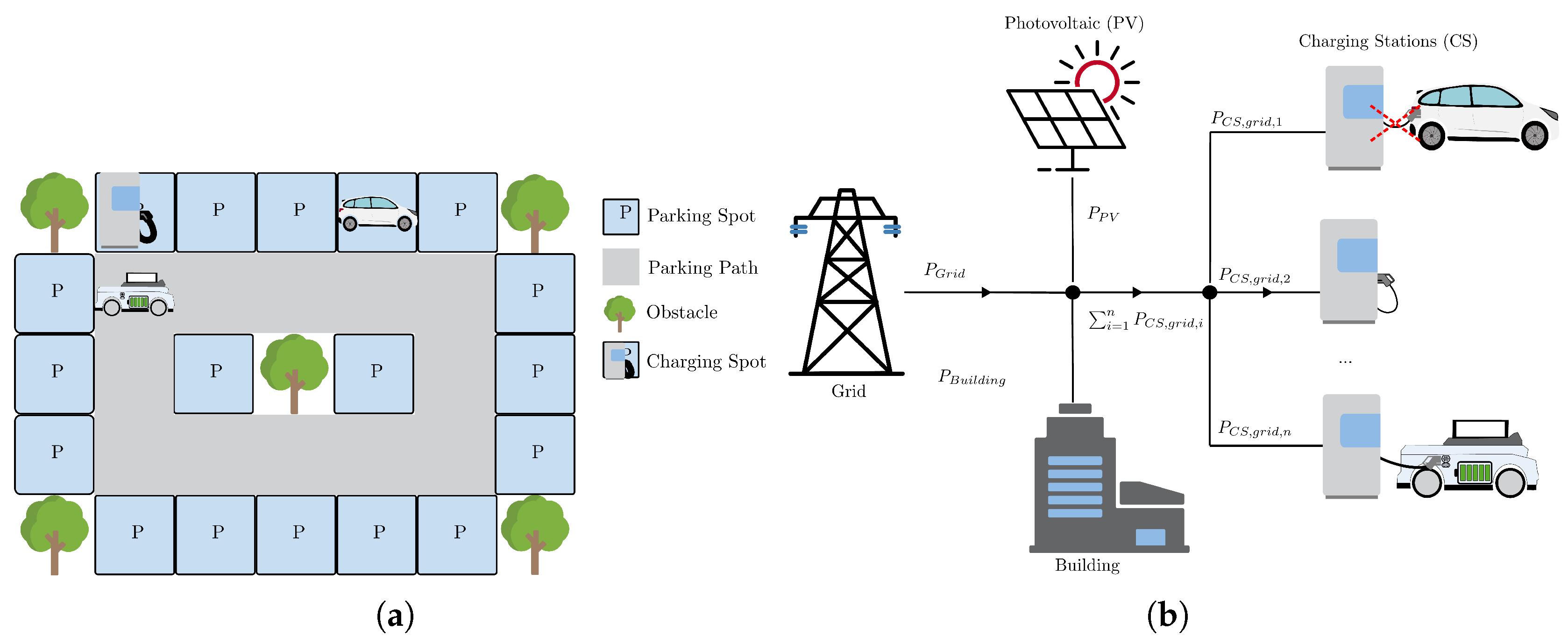
Figure 2.
MPC controller without forecast model and horizon of 96 steps (8 hours); (a) power contributions at charge point (b) accumulated cost and revenue (c) SoC of MCR (d) electricity price (e) number of EVs at charge point. Final profit €-15.29 (Cost €103.56 , Revenue €88.27 )
Figure 2.
MPC controller without forecast model and horizon of 96 steps (8 hours); (a) power contributions at charge point (b) accumulated cost and revenue (c) SoC of MCR (d) electricity price (e) number of EVs at charge point. Final profit €-15.29 (Cost €103.56 , Revenue €88.27 )
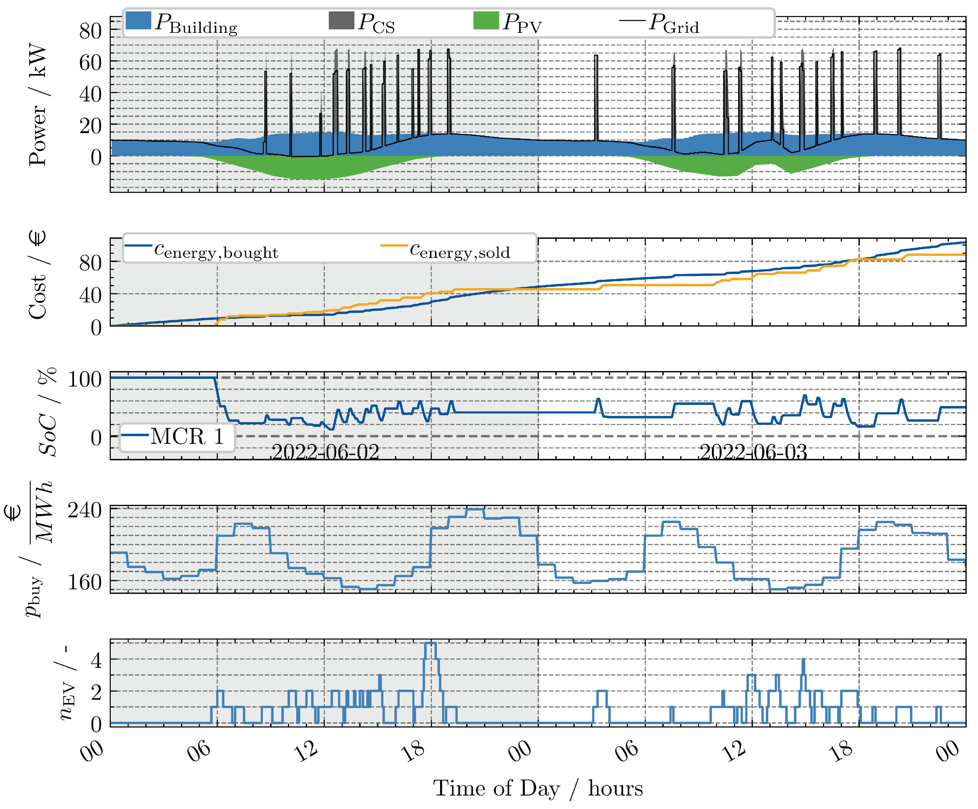
Figure 3.
Training Loss LSTM
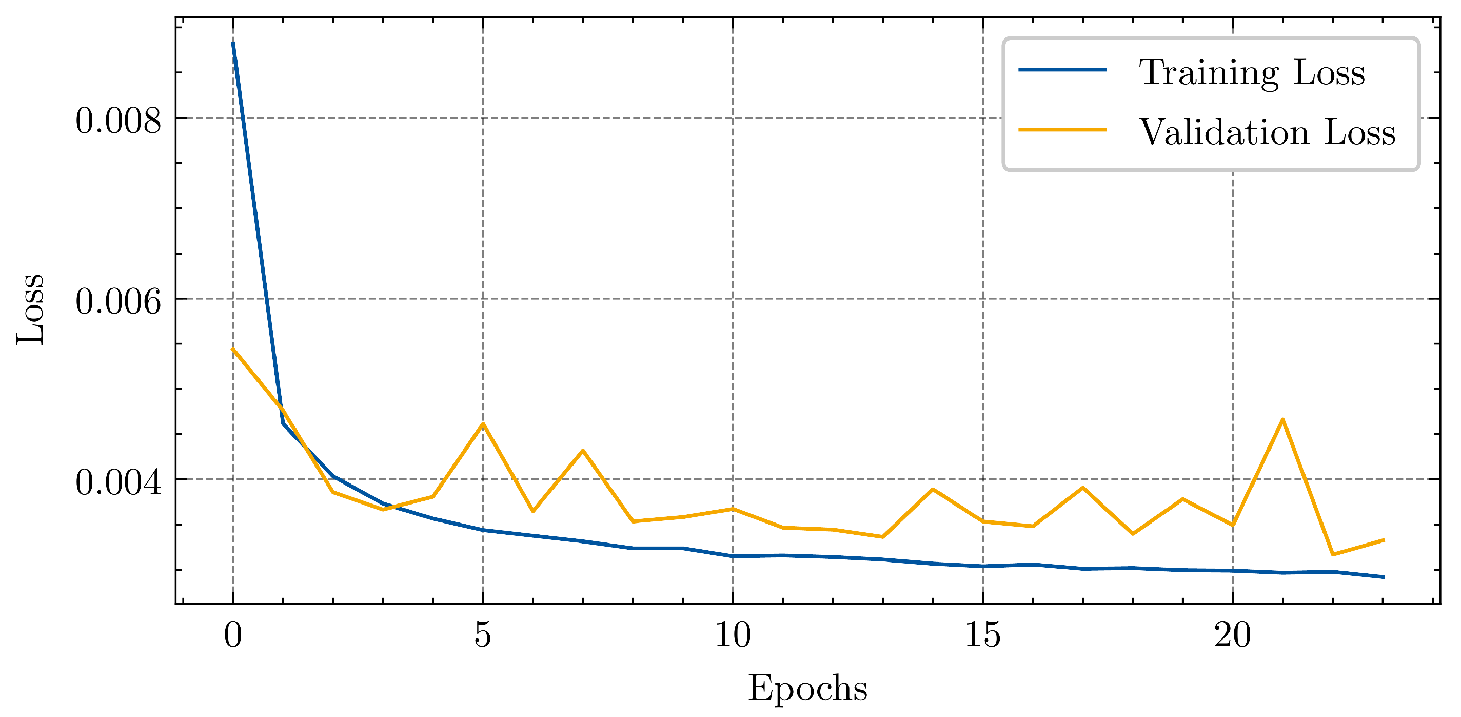
Figure 4.
Exemplary prediction with test set for ACN dataset with 8 hours of prediction horizon (a) Mo 24-02-2020 4:00 h - 12:00 h; (b) Mo 03-02-2020 06:00 h - 14:00 h; (c) Tu 21-01-2020 11:00 h - 19:00 h
Figure 4.
Exemplary prediction with test set for ACN dataset with 8 hours of prediction horizon (a) Mo 24-02-2020 4:00 h - 12:00 h; (b) Mo 03-02-2020 06:00 h - 14:00 h; (c) Tu 21-01-2020 11:00 h - 19:00 h
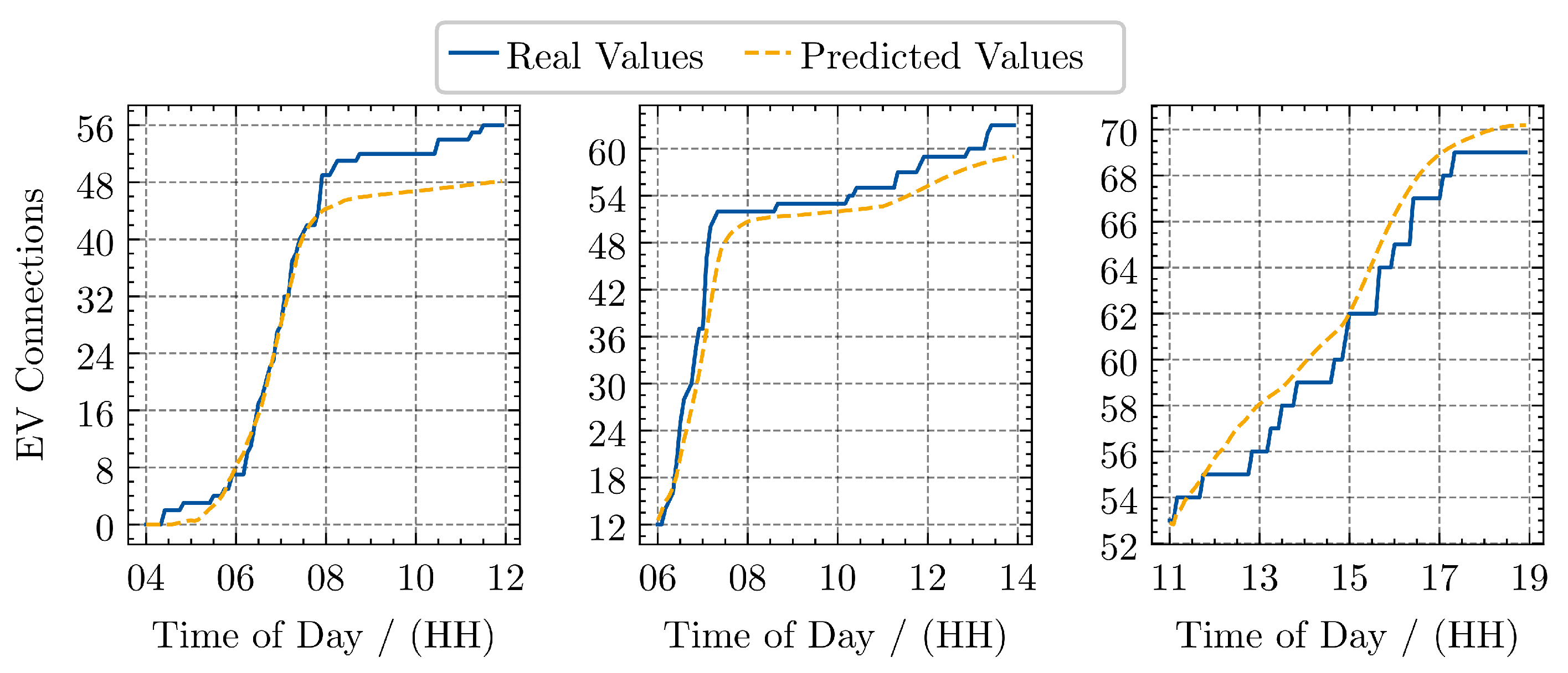
Figure 5.
Exemplary prediction with test set for synthetic supermarket dataset with 8 hours of prediction horizon (a) Fr 01-12-2023 4:00 h - 12:00 h; (b) Mo 07-12-2023 06:00 h - 14:00 h; (c) Sa 12-12-2023 11:00 h - 19:00 h
Figure 5.
Exemplary prediction with test set for synthetic supermarket dataset with 8 hours of prediction horizon (a) Fr 01-12-2023 4:00 h - 12:00 h; (b) Mo 07-12-2023 06:00 h - 14:00 h; (c) Sa 12-12-2023 11:00 h - 19:00 h
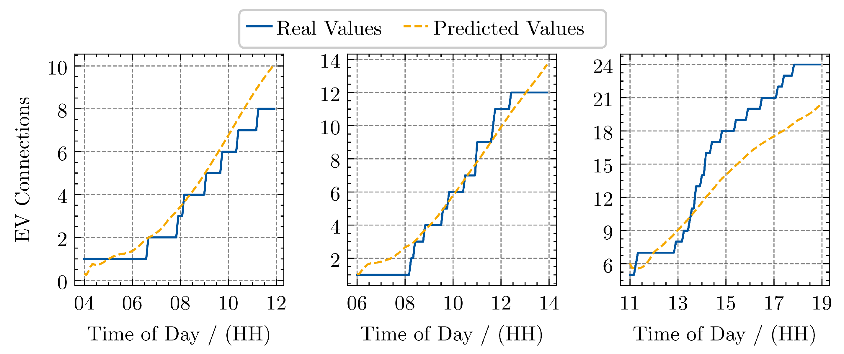
Figure 6.
Without explicit prediction, terminal cost - horizon 10 steps (50 minutes);(a) power contributions at charge point (b) accumulated cost and revenue (c) SoC of MCR (d) electricity price (e) number of EVs at charge point. Final profit €-1.15 (Cost: €116.26, Revenue: €115.11 )
Figure 6.
Without explicit prediction, terminal cost - horizon 10 steps (50 minutes);(a) power contributions at charge point (b) accumulated cost and revenue (c) SoC of MCR (d) electricity price (e) number of EVs at charge point. Final profit €-1.15 (Cost: €116.26, Revenue: €115.11 )
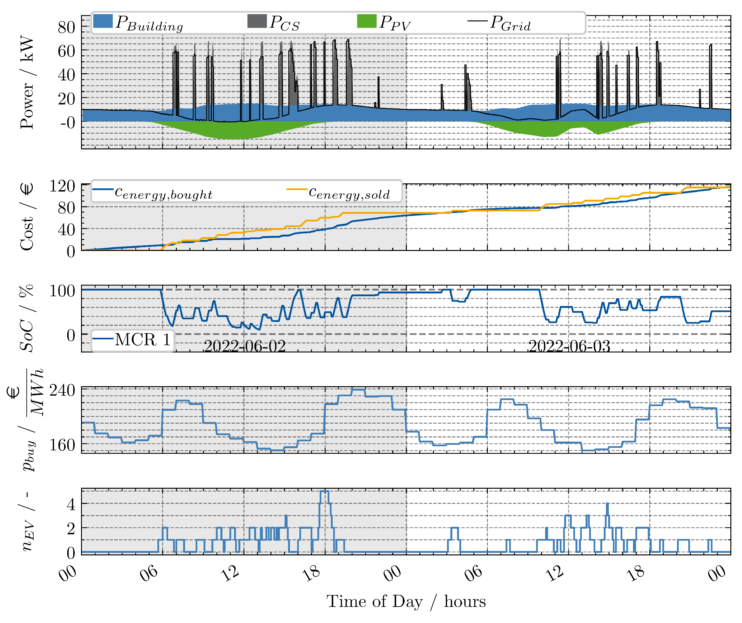
Figure 7.
MPC with perfect forecast and horizon of 96 steps (8 hours); (a) power contributions at charge point (b) accumulated cost and revenue (c) SoC of MCR (d) electricity price (e) number of EVs at charge point. Final profit €14.64 (Cost: €126.06, Revenue: €140.70 )
Figure 7.
MPC with perfect forecast and horizon of 96 steps (8 hours); (a) power contributions at charge point (b) accumulated cost and revenue (c) SoC of MCR (d) electricity price (e) number of EVs at charge point. Final profit €14.64 (Cost: €126.06, Revenue: €140.70 )
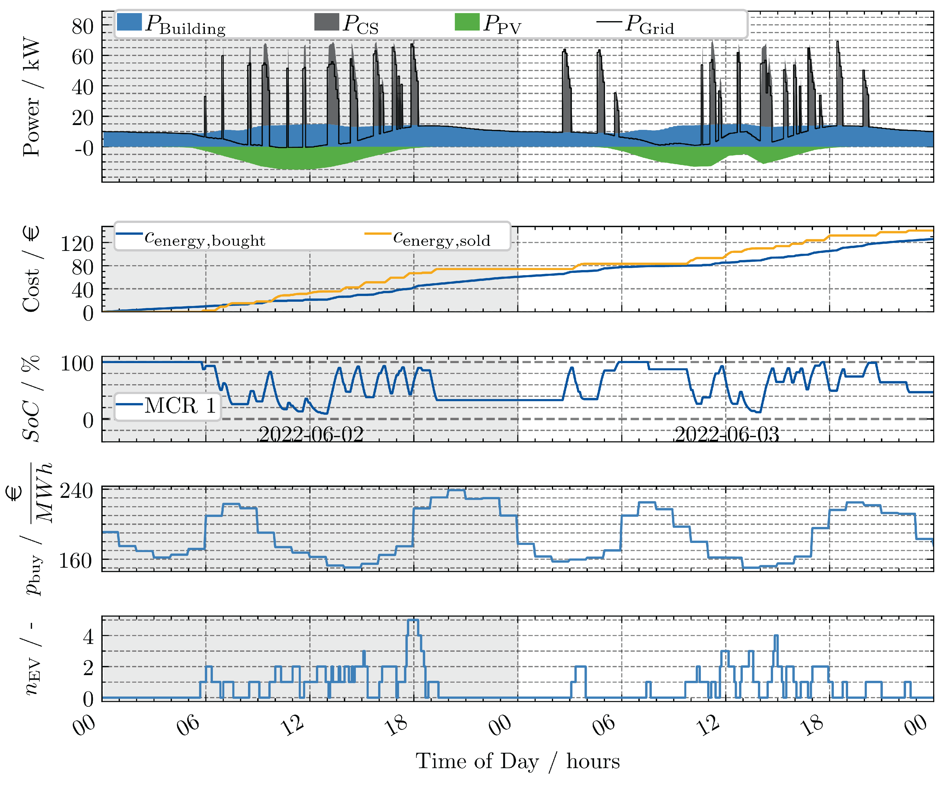
Figure 8.
LSTM Prediction with horizon of 96 steps (8 hours): (a) power contributions at charge point (b) accumulated cost and revenue (c) SoC of MCR (d) electricity price (e) number of EVs at charge point. Final profit: €7.85 (cost €124.71, revenue: €132.56)
Figure 8.
LSTM Prediction with horizon of 96 steps (8 hours): (a) power contributions at charge point (b) accumulated cost and revenue (c) SoC of MCR (d) electricity price (e) number of EVs at charge point. Final profit: €7.85 (cost €124.71, revenue: €132.56)
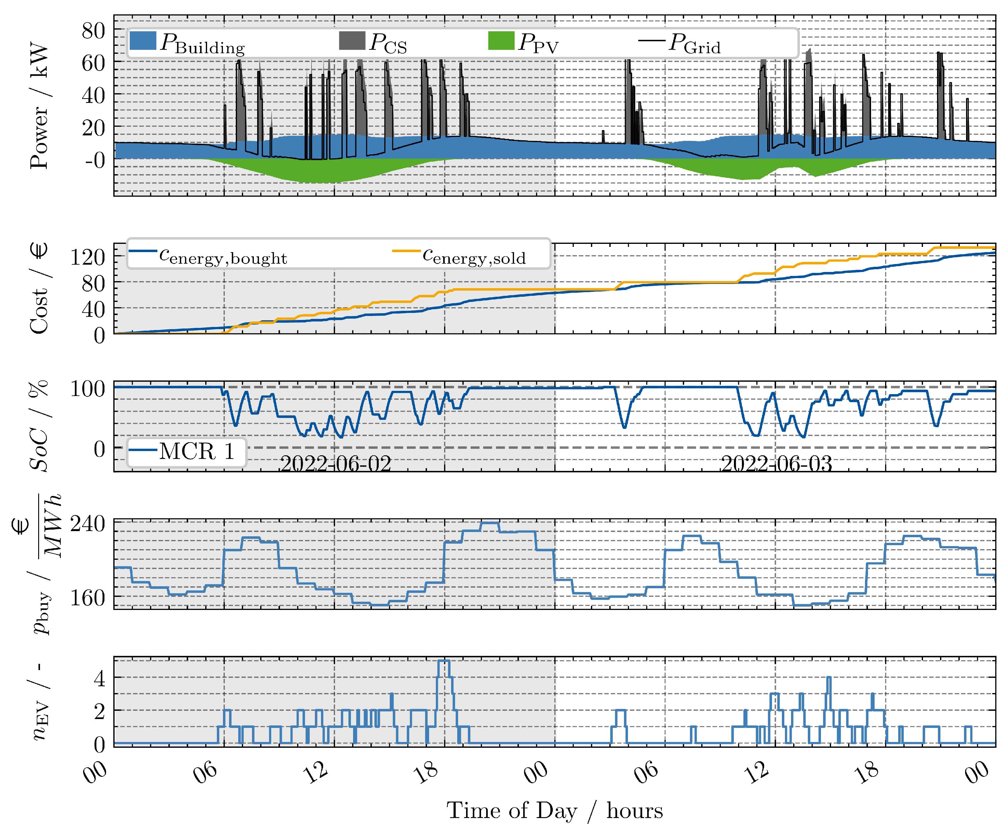
Table 1.
Environment configuration for analysis
| Parameter | Description | Value |
|---|---|---|
| Number of CS on parking area | 1 | |
| Maximum charging power of the CS | 50 kW | |
| Yearly consumption of supermarket building | 200000 | |
| Peak power of installed PV array | 20 | |
| Average arriving EVs per hour | 1 | |
| Number of MCR in the environment | 1 | |
| Number of parking fields in environment | 8 |
Table 2.
Input (x) and Output () from LSTM
| Variable | Raw Value | Processing | Processed Variable |
|---|---|---|---|
| Time of Day (ToD) | Sin/Cos Encoding: | , | |
| Day of Week (DoW) | Sin/Cos Encoding | , | |
| Accumulated arrived EVs | normalized accumulated arrived EVs | ||
| Accumulated arrived EVs | normalized accumulated arrived EVs |
Disclaimer/Publisher’s Note: The statements, opinions and data contained in all publications are solely those of the individual author(s) and contributor(s) and not of MDPI and/or the editor(s). MDPI and/or the editor(s) disclaim responsibility for any injury to people or property resulting from any ideas, methods, instructions or products referred to in the content. |
© 2025 by the authors. Licensee MDPI, Basel, Switzerland. This article is an open access article distributed under the terms and conditions of the Creative Commons Attribution (CC BY) license (http://creativecommons.org/licenses/by/4.0/).
Copyright: This open access article is published under a Creative Commons CC BY 4.0 license, which permit the free download, distribution, and reuse, provided that the author and preprint are cited in any reuse.


