
Submitted:
28 January 2026
Posted:
30 January 2026
You are already at the latest version
Abstract
To investigate the closedness of the universe, we introduce a novel theoretical model to explore its geometry, treating it as the crust of a four-dimensional sphere. Building upon the FLRW model and considering alternative cosmological scenarios, the study examines the motion of light in the fourth dimension to infer the universe's curvature. The approach involves mathematical modeling of spiral light trajectories, a theoretical framework for the nature of time across quantum and cosmic scales, and the determination of the universe's four-dimensional radius using Hubble's law. The model predicts the existence of mirror points and provides calculations of their positions relative to Earth under various parameters. The observational predictions calculated in this paper are measurable and verifiable.
Keywords:
closed universe
; mirror points
; fourth dimension
; light propagation
1. Introduction
This paper presents a theory and then examines its results by calculating the path of light in the fourth dimension. According to the FLRW (Friedmann-Lemaître-Robertson-Walker) model, if the density of the universe exceeds the critical density , then the universe is geometrically closed [1,2,3]. The current calculated value for is approximately equal to one [4]. Certain cosmological models, such as those involving phantom energy, inhomogeneous cosmological models, additional matter formation, backreaction models, and future evolution of the universe, suggest that the current estimates of the universe’s density may be incorrect or subject to revision [5,6,7,8,9,10,11,12,13,14,15,16,17,18,19,20,21,22,23,24,25,26,27,28,29,30,31,32,33,34,35,36,37,38]. This could be important given possible future refinements in calculating the density of the universe. This paper attempts to consider a general model for the closed universe that is consistent with previously validated models describing cosmic phenomena such as general relativity, Hubble calculations and cosmological measurements [39,40,41].
A three-dimensional sphere has a two-dimensional surface (or crust). Similarly, a circle is two-dimensional, with its circumference being one-dimensional. In general, the boundary, or crust, of an object is one dimension lower than the object itself. Therefore, the crust of a four-dimensional sphere is a three-dimensional object. For two-dimensional beings living on the two-dimensional surface of a three-dimensional sphere, their universe appears flat and cannot be curved from their perspective. If the universe is closed, it appears flat to us. In this paper, the closed universe is modeled as the crust of a four-dimensional sphere, with the time axis aligned parallel to the sphere’s radius. This paper proposes an approach to understanding the universe’s curvature by analyzing the motion of light in the fourth dimension [43].
To investigate the motion of light in the fourth dimension, it is necessary to model the spiral motion based on physical quantities. Therefore, Section 2.1 is dedicated to mathematical modeling. In Section 2.2 and Section 2.3, a coherent theory regarding the nature of time across quantum (small-scale) and cosmic (large-scale) dimensions is proposed, respectively. In Section 2.4, we evaluate the effect of gravity on space-time according to the presented model. In Section 2.5, the radius of the universe’s four-dimensional sphere by applying Hubble’s law is determined. Moreover, the theory proposed in this model predicts the existence of mirror points in the universe. In the results section, based on different values for the parameters in the model, the positions of the mirror points and the farthest points in space relative to the Earth have been calculated.
2. The Model
2.1. Modeling Spiral Motion
In this section, we introduce a model for generating spiral motion in two dimensions. We assume that an object moves on a circle with a constant velocity B. Simultaneously, the radius of the circle increases over time at a constant rate V. To derive the equation of motion for this object, we first compute its angular velocity as follows:
where R(t) represents the radius of the circle as a function of time:
The angular displacement of the object can be obtained by integrating the angular velocity with respect to time, given by:
Utilizing Equations (2) and (3), we derive the parametric form of the object’s equations of motion as follows:
The polar equation for the golden spiral is as follows [42]:
where is the golden ratio. To facilitate a clearer comparison with equations (4) and (5), and to enable more effective plotting, we express equation (6) in its parametric form:
Now we present plots of the object’s equation of motion at a constant velocity V=1 across varying speeds of parameter B, compared to the golden spiral depicted in Figure 1, and this demonstrates that when the ratio of the velocity of B to V is equal to , the resulting pattern closely approximates the Fibonacci golden spiral. Additionally, observing the diagrams from left to right in Figure 1, it is evident that increasing the velocity of B results in a greater curvature in the object’s motion. The key condition to demonstrate that an equation of motion describes a golden spiral is as follows [42]:
To verify condition (9) for Equations (4) and (5) at and , we select the arbitrary points as illustrated in Figure 2 (left). Also equation (9) was analyzed for the case where B and V are both equal to one. In this scenario (B=V), the result of the equation (9) is equal to 4.8. Consequently, for B=V=1, the equation of motion can be expressed in Figure 2 (right):
The Table 1 presents the specifications of the four selected points from Figure 2 (left), which are located along the object’s path, along with an review of Condition (9) as follows:
As shown in Table 1, the ratios obtained from the points are close to the value of . Therefore, in future calculations, we will employ Equations (4) and (5), using the velocity ratio for calculation on the Golden Spiral.
In the following section, we will explore the mechanisms of time at both the quantum (small-scale) and cosmic (large-scale) levels.
2.2. The Mechanism of Time
This section introduces a model for the nature of time. While the universe is typically described in three spatial dimensions, with time as the fourth perpendicular dimension, we simplify our discussion by considering space as one-dimensional for clarity.
According to Figure 3, consider two objects, A and B, moving through space. Object A moves at a slow velocity, while object B travels at the speed of light. Consequently, the smallest particles of object B cover a distance of one Planck length in each Planck time interval. In contrast, this is not the case for object A, whose particles move much more slowly.
As shown in Figure 3, in this model, the 3D crusts in the fourth dimension that are parallel to each other. The smallest volume in the universe is a cube with a side length of one Planck length. A quantum model for the nature of time is proposed, where the information of each cube at a given Planck time is transferred to the next crust via an intermediate particle, which we have named Y. When an object moves faster, its movement in the fourth dimension becomes more inclined because the information of each cube associated with that object is transferred to the neighboring cube in the subsequent crust. The oblique motion of light in the fourth dimension results from its extremely high speed. Consequently, the angle formed during this motion corresponds to the angle within Einstein’s light cone. Since no particle can travel faster than the speed of light, information from a cube in one crust cannot be transmitted to more distant cubes in the next crust. This limitation can be exemplified by the restricted interaction of the intermediate particle Y, similar to the asymptotic freedom observed in gluons. Just as a gluon transfers color charge between quarks, a hypothetical Y particle could transfer information between two parallel crust. This information can be considered the smallest unit of energy, with the arrangement of these fundamental units giving rise to various basic structures. It is possible that an object’s high kinetic energy can trigger the activation of oblique movement of the intermediate particle Y. The size of particle Y in Figure 3 is hypothetical, and this particle functions as an intermediary between two parallel spaces, characterized by a metric distinct from that of conventional space.
In this work we adopt a minimal and conservative realization of the mediator Y as a gauge-singlet scalar field whose coupling to the local information current is modulated by a preferred timelike background . This choice preserves local gauge invariance of the Standard Model sector, keeps the field-theoretic structure simple, and allows a clear implementation of one-way (past→future) information transfer via retarded propagation. We take the mediator Y to be electrically neutral (a gauge singlet) to avoid direct minimal couplings to Standard Model gauge fields. This choice simplifies the effective action and greatly reduces experimental and cosmological constraints, allowing us to focus on the information-transfer phenomenology. The effective Lagrangian used in the main text is
when varying the action one must account for boundary terms arising from the derivative coupling ; here we assume either compact support for variations or boundary conditions that render these surface terms negligible. The Lagrangian is invariant under Standard Model gauge transformations and under spatial rotations in the rest frame defined by . In Equation (10) denotes the local scalar density of the Planck-cube information, is a unit timelike vector field selecting the local time direction, and is an effective, energy-dependent coupling. In natural units () the interaction term must have mass dimension four, with , and , one finds . The factor ensures that the coupling is sensitive to the local temporal flow and therefore to the sign of time derivatives, while the use of the retarded Green’s function for enforces causality and one-way information transfer. At the beginning of Section 2.2, we explained how a suitable choice of reproduces the phenomenology: for low local kinetic energy K, the effective radial transfer is negligible (near-orthogonal transfer), whereas as K approaches relativistic values, the coupling increases and the effective inclination of information transfer approaches the light-cone limit (). Full propagator expressions and numerical estimates are given in Appendix A.
We note that imposing a single-tick (Planck-time) activation of the mediator naturally places its characteristic mass at the Planck scale. Requiring the Compton time to be of order yields . This choice confines the mediator’s temporal dynamics to the Planck tick and, together with an effective damping , strongly suppresses propagation beyond the immediately subsequent crust. Because in this regime approaches the quantum-gravity scale, we treat the present construction as an effective parametrisation valid up to a Planck cutoff and explicitly state the associated caveats (see Appendix B). The characteristics of the Y particle, as obtained from the calculations in Section 2.2, are shown in Table 2.
2.3. General Relativity
In our model the of the hypersphere is identified with the cosmological scale factor. We therefore adopt the closed FLRW line element and set the scale factor [49]. The present treatment is an effective description valid up to a Planck cutoff; when mediator parameters approach the Planck scale we explicitly note the limitations of the EFT. Below we give the metric, the relevant geometric quantities, the Einstein equations in Friedmann form, and short guidance on how to include the model’s matter / mediator contributions in the stress–energy tensor. Appendix C collects the retarded-propagator remarks together with the full set of intermediate geometric expressions for reproducibility: Christoffel symbols, Ricci tensor and scalar, and the complete Einstein tensor.
Metric and Identification
We use signature and coordinates . The closed FLRW metric reads In the text we therefore identify the model radius with the cosmological scale factor: .
Energy–Momentum Ansatz
As a first, minimal choice we model the matter content by a perfect fluid (or by effective fluid components that collect contributions from fields in the model):
The matter content is modelled as an effective perfect fluid with energy density and pressure . If the mediator field contributes dynamically, its homogeneous energy density and pressure (spatially averaged on scales larger than the crust microstructure) are [46,47]
and one sets , .
Key Geometric Identities (Compact Form)
For the metric above the nonzero Christoffel symbols relevant to the homogeneous dynamics include
and the Ricci components and scalar reduce (for the homogeneous background) to
where denotes the metric on the unit 3-sphere and spatial indices run over .
Einstein Equations and Friedmann Form
The Einstein field equations with cosmological constant are
For the closed FLRW metric these reduce to the Friedmann equations
together with the continuity equation (consequence of ):
These equations determine the dynamics of once and are specified.
How to Include Model Components in
Below are three practical options; choose the one that best matches the physical interpretation you adopt in the manuscript.
- 1.
- Effective perfect fluid. Treat the crust and its internal degrees of freedom as an effective homogeneous fluid with and . Insert these into the Friedmann equations and solve for .
- 2.
- Explicit scalar mediator contribution. If the mediator is dynamical and approximately homogeneous on cosmological scales, include and given above. If is strongly localized to crust microstructure, average appropriately and include only the coarse-grained contribution.
- 3.
- Shell / embedding effects. If the 3-dimensional crust is best modelled as a thin shell embedded in a higher-dimensional geometry, use Gauss–Codazzi relations and Israel junction conditions to derive an effective surface stress tensor that modifies the 4D dynamics (see Appendix C).
Remarks on Interpretation and Validity
- Identifying places the model squarely within standard cosmology for a closed universe; this allows direct comparison with observational constraints once and p are specified.
- The presence of a preferred timelike background explicitly breaks boost invariance; experimental constraints on Lorentz violation summarized in the Standard-Model Extension (SME) literature require that any low-energy Lorentz-violating effects be sufficiently suppressed, and we therefore assume such effects are Planck-suppressed or otherwise below current bounds [44].
- If mediator parameters or masses approach the Planck scale, the effective field theory treatment must be qualified: state explicitly any Planck cutoff and the regime of validity.
- If the crust carries intrinsic surface energy or tension, the embedding / junction approach is recommended to capture extrinsic curvature effects.
If the density of the universe exceeds from the critical density, then the universe is closed. In this case, the three-dimensional space of the universe can be thought of as a crust of four-dimensional sphere. Because Figure 3 depicts a very small scale, this curvature is not readily apparent.
However, in Figure 4, which illustrates the universe on a larger scale, the curvature of this space crust is visible as part of the encompassing four-dimensional sphere.
As illustrated in Figure 4, the light traveling from a galaxy to Earth follows the curved path marked in red, rather than the green path.
Therefore, the oblique motion of light in the fourth dimension at the quantum scale results in a corresponding oblique motion of light at the cosmic scale.
2.4. The Effects of Gravity on Spacetime
This section explores how gravity influences time. According to Figure 5, if we consider that the crust of three-dimensional space is curved along the time axis by placing a massive celestial body in space, then this crust expands towards the center of the four-dimensional sphere. This means that objects near this massive celestial body, are behind in time than other objects on this crust.
In Figure 5, we assume that a black hole is created in space at time (R) after the Big Bang (W) and disappears at time (P). In this case, the black hole bends spacetime around itself, which brings the crust closer to the center of the sphere. This causes time to run slower for objects near the black hole.
2.5. Evaluating Light Curvature
In this section, the motion of light on the surface of a growing four-dimensional sphere is evaluated based on the equations obtained from the Section 2.1. First, the current crust expansion rate is measured. So the arc length of a growing circle with radius and central angle is given by . Therefore, the crust growth rate is calculated as follows:
therefore, the farther an object is from Earth, the greater its escape velocity, since it subtends a larger central angle. So if we equate this relationship with Hubble’s relationship, we can calculate the radius of the four-dimensional sphere. If we assume that an asteroid is located one light year from Earth, its escape velocity from Earth for is given by the following equation:
Since the value of is equal to one light year, we obtain the radius of the four-dimensional sphere by equating equations (18) and (19), as follows:
The radius of the universe’s four-dimensional sphere for different parameter changes is calculated, as illustrated in the Table 3.
In Table 3, the values are in (). Also, the pertains to the golden spiral described in Section 2.1 and indicates the behavior of light traveling in the fourth dimension as modeled based on golden spiral. While the unit of R in Table 3 is the light year, it represents the axis of the fourth dimension, which, as shown in Figure 4, is perpendicular to space. Therefore, R effectively corresponds to a measure of time, with the unit of years. Therefore, the values in Table 3 represent the age of the universe corresponding to various parameter changes. The green cell in the Table 3 indicates the value closest to the measured age of the universe [41].
There are points in the four-dimensional space-time sphere of the universe that have two properties: first, they have a phase difference with respect to the Earth equal to integer multiples of , and second, if light emerges from the points of this spatial crust, it reaches Earth in current crust according to the path of the light spiral. To simplify notation, I have named these points "mirror points". For this reason, these points are named ’mirror points,’ because when a person stands between two mirrors, he can see both front and behind of himself simultaneously. In Figure 6, we depict the position of the first mirror point relative to Earth, based on calculations performed with Mathematica.
In Figure 6 (left), two light rays originating from a celestial body in the ancient crust (blue) are illustrated. The age of this crust is about 606 million years after Big Bang, determined from the universe’s age, which is indicated in green in Table 3. In fact, a powerful space telescope capable of zooming this far could capture images of the celestial object from two different perspectives: one from the front and another from the behind of the celestial object.
In Figure 6 (right), we have placed a hypothetical cube at a mirror point, on each face of this cube, the letters A, B, C, D, E and F are written. If a telescope in Earth’s orbit observes such a distance, depending on the telescope orientation position, it will see a different letter from this cube. In other words, by rotating the telescope around itself, it can see the image of the rotation of the cube.
Now we want to find the number of rotation of light within the four-dimensional sphere of the universe that it has traveled to reach us from one year after the Big Bang to the present.
In Figure 7, points C and E are mirror points, while point A has a phase difference of relative to point E. When zooming in graph, you’ll notice that the same shape is drawn inward from E point, creating a repeating pattern to inner. Using the plotting tool in Mathematica, The R ratios were calculated for the points in the Figure 7 until the approached 1. The corresponding values of these ratios are determined as follows:
The number of cycles observed with the drawing tool in Mathematica ranged from 3 to 4 cycles. However, to precisely determine its value, we apply Equation (21) as follows:
If we consider to represent one year after the Big Bang, then the number of cycles for become =(3.722). Since the number of mirror points is twice the number of rotations (excluding point A itself), the total number of mirror points at these parameter values is 7.
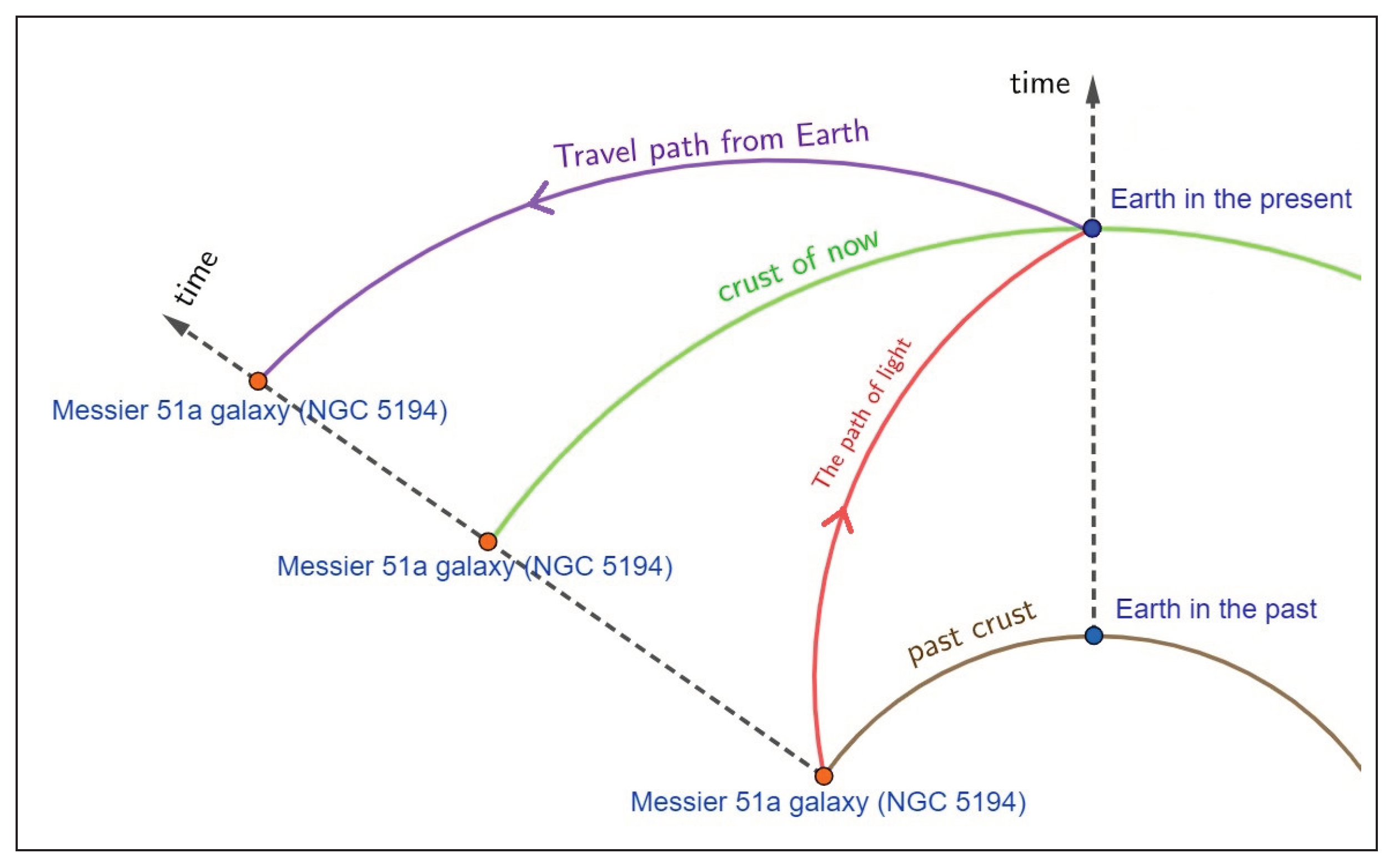
According to Figure 8, the brown, red, green, and purple arcs represent the spatial distance between Earth (when light from the galaxy began to radiate) and the Messier 51a galaxy, the path that the light from the Messier 51a galaxy traveled in the fourth dimension to reach Earth, the spatial distance between Earth (when light was received) and the Messier 51a galaxy, the distance that a person from Earth would have to travel at the speed of light to reach the Messier 51a, respectively. The brown path represents the distance used by astronomers as the criterion for an object’s distance from Earth, while the green path is the object’s actual distance from Earth.
The measured distance of the Messier 51a galaxy from Earth is 23.5 million light years (brown path), so the distance between Earth in the present and Earth in the past is 23.5 million years (dashed line). Table 4 lists the actual distance from Earth to Messier 51a (green path) and the light-speed travel distance to reach this galaxy for .
As shown in Table 4, Messier 51a galaxy is approximately 39,000 light-years farther away than it appears. If the angle between a celestial body and the Earth on the 4D sphere exceeds , the body approaches the Earth from the opposite side of the 4D sphere. Consequently, it is possible for the body’s position to coincide with the Earth’s current location but at a past time, causing the length of the green curve to be zero. This would imply that the body was at Earth’s present location before the Earth formed or reached its current position.
In the following section, we determine the number of mirror points and their respective locations for various parameter values within the model.
3. Results
In the previous section, we did not analyze the model for values of R less than one year, because, in the early stages of the universe, light had enough time to traverse the crust of entire four-dimensional sphere of the cosmos within just a few years. This greatly increased the likelihood of photons colliding with matter, making it improbable for us to observing the universe’s earliest moments. According to this model, the early universe remains invisible to our eyes appearing dark and yet is exceedingly luminous from itself perspective.
In Table 5 the age of the mirror points by year () are calculated based on different values of the universe age, which are given in Table 3 and the calculations in Section 2.5.
For Table 5, we selected only those values of the universe age from Table 3, that are not inconsistent with cosmological observations and less than 13 billion years. As can be seen in Table 5, the density of mirror points is higher in the early times. And light has performed most of its cycles in the beginning of the universe.
Since if we move in a closed universe in one arbitrary direction at a speed in a straight line, after a while we will return to our original position from the opposite direction, therefore the point on the current crust that is farthest from Earth () in 3D space, lies beyond the four-dimensional sphere, and its distance from Earth is . This means that if an object moves in a straight line through space at a constant speed, it will approach the Earth when it passes this point (). This means that space is closed. The volume of the current universe () can be obtained from surface area of 4D sphere . But, the volume of 4D sphere () is obtained from the formula , which represents the total volume of the universe’s spacetime [43]. All the values resulting from these calculations are given in Table 6:
4. Conclusion
In this paper, a suitable physical modeling was obtained for the golden spiral and the movement of light at (B=V). The presented model aligns well with Einstein’s light cone concept and accurately reflects the influence of gravity on spacetime within the framework of general relativity. The presented model effectively bridges the concept of time at both the quantum (small-scale) and cosmic (large-scale) levels. Since hypothetical particles Y are exchanged between two parallel universes, they can be interpreted as a new force that holds the two planes of the universe together. According to the values obtained from Table 3, it can be concluded that the idea of light moving in the fourth dimension according to the golden spiral is not correct. Rather, light moves in the fourth dimension at (B=V). This conclusion is reinforced by the correlation between the values in Table 3 and the observed measurements of the universe’s age. The mechanism of expansion of the space-time crust in this model is in good agreement with the Hubble’s law. The model presented in this paper predicts mirror points, which will make this model verifiable. According to Table 4, celestial objects with angles to Earth less than are farther away than their apparent distances suggest. The verification of this model involves observing that when a powerful telescope looks at celestial body located at mirror points positions relative to Earth, the images of celestial body will rotate accordingly as the telescope rotates around its own axis.
Data Availability Statement
The Mathematica files and data supporting the results are available at here.
Appendix A. Retarded Propagator
(Retarded propagator, Compton wavelength and sample coupling)
Appendix A.1. Retarded Propagator for a Massive Scalar
The retarded Green’s function for a massive scalar field in flat spacetime (on a quantum scale for particle Y) is defined by
In momentum space the retarded propagator is written as
with the prescription enforcing the retarded boundary condition. For a spatial separation r and time difference the propagator contains the causal support inside the light cone and, for , exhibits Yukawa suppression . In the layered crust picture the amplitude for information transfer between adjacent crusts separated by is proportional to
evaluated with and for nearest-neighbour transfer.
Note that, by the local flatness theorem, the flat-space retarded Green’s function used in Appendix A provides a valid order-of-magnitude approximation for mediator propagation whenever the relevant wavelengths and separations satisfy . In our benchmark choices ( and ) this condition holds and the flat approximation is justified.
Appendix A.2. Compton Wavelength and Order of Magnitude Estimates
The Compton wavelength of the mediator sets the effective radial range of transfer:
Using the Planck length and the Planck mass (equivalently ), one finds
so that choosing confines transfer essentially to the same Planck cube or immediate neighbour, while somewhat below allows coupling across a few adjacent crusts. The Yukawa suppression factor for separation is
giving for and for .
Appendix A.3. Sample Energy Dependent Coupling
To model the observed phenomenology that higher local kinetic energy K increases the inclination of transfer, we introduce a smooth, bounded coupling
with a convenient choice
or, if a sharper threshold is desired,
where is the characteristic kinetic energy scale (e.g. a fraction of the local rest energy) and controls the steepness. With these choices (negligible coupling at low kinetic energy) and for (saturated coupling at high kinetic energy). The effective discrete radial step introduced in the main text can be parametrized as
and the inclination angle follows from the discrete relation
so that for and one recovers ().
Appendix A.4. Numerical Example
Choose representative parameters , , equal to the rest energy scale of the Planck cube and . For a near-lightlike local motion we have and , giving . For nonrelativistic the coupling is suppressed and , yielding . These order-of-magnitude estimates demonstrate that the scalar + timelike background construction can reproduce the desired two-regime behaviour while remaining minimal and gauge-safe. Detailed numerical integration of in the curved embedding metric and a full parameter scan are left to future work and can be provided on request.
Appendix B. Mass and Temporal Damping of the Mediator ϕ Y
The requirement that the mediator Y transfers information only to the immediately subsequent time crust (separation ) constrains its characteristic temporal scales. Two quantities control the temporal behaviour: the Compton time
and an effective damping (width) that parametrises temporal suppression of propagation between ticks. Requiring that the field be active on the single-tick timescale but suppressed for multi-tick transfer leads to the order-of-magnitude conditions
Using gives , i.e. (Planck mass). Numerically,
With the temporal suppression factor per tick is , and for two ticks , so transfer beyond the nearest neighbour is strongly suppressed.
In a simple effective description one may include the damping by promoting the mass term to a complex pole in the retarded propagator. The retarded Green’s function in momentum space then reads
and causal support is preserved by the prescription. For nearest-neighbour transfer we evaluate the amplitude with and set by the layered geometry; the Yukawa-like temporal/spatial suppression ensures negligible amplitude for when and .
Caveat.
Choosing and in the Planck regime places the mediator in the domain where quantum gravitational effects may be important; the present effective treatment should therefore be regarded as a phenomenological parametrisation valid up to the Planck cutoff.
Appendix C. Geometric Derivations
(geometric derivations, Gauss–Codazzi and Israel junctions)
Appendix C.1. Full Geometric Components
We use the closed FLRW metric with scale factor :
Nonzero Christoffel Symbols
The nonvanishing Christoffel symbols (coordinate basis) are
Ricci Tensor Components
For the homogeneous background the nonzero components of the Ricci tensor are
Ricci Scalar
The Ricci scalar is
Einstein Tensor Components
The Einstein tensor has the nonzero background components
Checks and remarks
- Substituting into Einstein’s equations yields the Friedmann equation
- The spatial components above are related to the acceleration equation and reproduce
- The listed Christoffel symbols, Ricci components and Einstein tensor are the standard background expressions for the closed FLRW metric; they can be reproduced symbolically (e.g. with Mathematica/Maple/Sage) by inputting the metric .
Appendix C.2. Full Christoffel, Ricci and Einstein Tensor (Background)
The full set of nonzero Christoffel symbols, Ricci tensor components and the Einstein tensor for the metric can be generated symbolically (e.g. with Mathematica or Maple) [48]. For reproducibility we list the background results used in the main text:
Substituting into Einstein’s equations yields the Friedmann equations quoted above.
Appendix C.3. Gauss–Codazzi and Israel Junction Conditions (Shell Embedding)
If the 3-dimensional crust is treated as a thin shell embedded in a higher-dimensional manifold, the intrinsic and extrinsic geometry are related by Gauss–Codazzi:
where is the extrinsic curvature of the shell and are tangent vectors. The Israel junction conditions for a thin shell with surface stress tensor read [45]
where denotes the jump of extrinsic curvature across the shell. These relations allow one to derive an effective surface energy–momentum contribution and to compute its backreaction on the bulk Friedmann dynamics. For a spherically symmetric shell the algebra simplifies and one obtains modified Friedmann equations with surface terms.
Implementation Notes
- To reproduce the intermediate symbolic steps, run a symbolic CAS (Mathematica, Maple, or Sage) on the metric and export the Christoffel, Ricci and Einstein tensors.
- If you adopt the embedding / junction approach, state the higher-dimensional background explicitly (ambient metric) and compute the extrinsic curvature for the chosen embedding surface.
- When comparing with observations, convert to conventional cosmological units (Mpc, Gyr) and compute standard observables (Hubble parameter , comoving distance, angular diameter distance).
References
- Friedman, A. Z. Phys. 1922, 10, 377–386. [CrossRef]
- Lemaitre, G. Nature. 1931, 127, 706. [Google Scholar] [CrossRef]
- Peebles, P. J. E. Princeton University Press, 2020, ISBN 978-0-691-20981-4.
- Aghanim, N.; et al. [Planck], Astron. Astrophys. A6 [erratum: Astron. Astrophys. 652 (2021);[astro-ph.CO]. 2020, arXiv:1807.06209641, C4. [Google Scholar] [CrossRef]
- Nojiri, S.; Odintsov, S. D. Phys. Rept [gr-qc]. 2011, arXiv:1011.0544505, 59–144. [CrossRef]
- Buchert, T. Gen. Rel. Grav. arXiv [gr-qc]. 2000, arXiv:gr32, 105–125. [Google Scholar] [CrossRef]
- Harlow, D.; Usatyuk, M.; Zhao, Y. arXiv [hep-th]. arXiv:2501.02359.
- Suvorov, A. G. Phys. Rev. D [gr-qc]. 2025, arXiv:2412.06696111(no.2), 023508. [CrossRef]
- Kamionkowski, M.; Toumbas, N. Phys. Rev. Lett. 1996, 77, 587–590. [CrossRef] [PubMed]
- Bamba, K.; Capozziello, S.; Nojiri, S.; Odintsov, S. D. Astrophys. Space Sci. [gr-qc]. 2012, arXiv:1205.3421342, 155–228. [CrossRef]
- Celerier, M. N. Astron. Astrophys. [astro-ph]. 2000, arXiv:astro353, 63–71. [Google Scholar]
- Linde, A. D. [arXiv:hep-th/0211048 [hep-th]].
- Alnes, H.; Amarzguioui, M.; Gron, O. Phys. Rev. D 2006, 73, 083519. [CrossRef]
- Bolejko, K.; Celerier, M. N.; Krasinski, A. Class. Quant. Grav. [astro-ph.CO]. 2011, arXiv:1102.144928, 164002. [Google Scholar] [CrossRef]
- Rasanen, S. JCAP [astro-ph]. 2006, arXiv:astro11, 003. [CrossRef]
- Cespedes, S.; de Alwis, S. P.; Muia, F.; Quevedo, F. Phys. Rev. D [hep-th]. 2021, arXiv:2011.13936104(no.2), 026013. [CrossRef]
- Ratra, B. Phys. Rev. D [astro-ph.CO]. 2017, arXiv:1707.0343996(no.10), 103534. [CrossRef]
- Nappi, C. R.; Witten, E. Phys. Lett. B [hep-th]. 1992, arXiv:hep293, 309–314. [CrossRef]
- Clarkson, C.; Ellis, G.; Larena, J.; Umeh, O. Rept. Prog. Phys. [astro-ph.CO]. 2011, arXiv:1109.231474, 112901. [CrossRef]
- Guth, A. H.; Steinhardt, P. J. Spektrum Wiss 1984, 7, 80–94.
- Dabrowski, M. P.; Stachowiak, T.; Szydlowski, M. Phys. Rev. D [hep-th]. 2003, arXiv:hep68, 103519. [CrossRef]
- Dutta, S.; Maor, I. Phys. Rev. D [gr-qc]. 2007, arXiv:gr75, 063507. [CrossRef]
- Weinberg, S. John Wiley and Sons; 1972; ISBN 978-0-471-92567-5, 978-0-471-92567-5. [Google Scholar]
- Caldwell, R. R.; Kamionkowski, M.; Weinberg, N. N. Phys. Rev. Lett. 2003, 91, 071301. [CrossRef]
- Kolb, E. W.; Turner, M. S. Front. In Phys.; Taylor and Francis, 1990; Volume 69, pp. 1–547. ISBN 978-0-429-49286-0, 978-0-201-62674-2. [Google Scholar] [CrossRef]
- Ford, L. H. Phys. Rev. D 1976, 14, 3304–3313. [CrossRef]
- Ellis, G. F. R.; P. McEwan, W. R.; Stoeger, S.J.; Dunsby, P. Gen. Rel. Grav. [gr-qc]. 2002, arXiv:gr34, 1461–1481. [CrossRef]
- Vogelsberger, M.; Genel, S.; Springel, V.; Torrey, P.; Sijacki, D.; Xu, D.; Snyder, G. F.; Nelson, D.; Hernquist, L. Mon. Not. Roy. Astron. Soc. [astro-ph.CO]. 2014, arXiv:1405.2921444(no.2), 1518–1547. [CrossRef]
- Nojiri, S.; Odintsov, S. D. eConf C0602061 [hep-th]. 2006, arXiv:hep06. [CrossRef]
- Handley, W. Phys. Rev. D [astro-ph.CO]. 2021, arXiv:1908.09139103(no.4), L041301. [CrossRef]
- Gratton, S.; Lewis, A.; Turok, N. Phys. Rev. D 2002, 65, 043513. [CrossRef]
- S. Kalyana Rama. Phys. Lett. B [hep-th]. 1999, arXiv:hep457, 268–274. [CrossRef]
- Burgarth, D.; Facchi, P. arXiv [quant-ph]. arXiv:2506.03254.
- Sami, M.; Toporensky, A. Mod. Phys. Lett. A [gr-qc]. 2004, arXiv:gr19, 1509. [CrossRef]
- Lesgourgues, J.; Tram, T. JCAP [astro-ph.CO]. 2014, arXiv:1312.269709 032. [CrossRef]
- Cline, J. M.; Jeon, S.; Moore, G. D. Phys. Rev. D [hep-ph]. 2004, arXiv:hep70, 043543. [CrossRef]
- Carr, B. J.; Kohri, K.; Sendouda, Y.; Yokoyama, J. Phys. Rev. D [astro-ph.CO]. 2010, arXiv:0912.529781, 104019. [CrossRef]
- Bezerra, V. B.; Klimchitskaya, G. L.; Mostepanenko, V. M.; Romero, C. Phys. Rev. D 2011, 83, 104042. [CrossRef]
- A. Einstein. Annalen Phys. 49 (1916)(no.7), 769–822. [CrossRef]
- Hubble, E. Proc. Nat. Acad. Sci. 1929, 15, 168–173. [CrossRef] [PubMed]
- Spergel, D. N.; et al. [WMAP]. Astrophys. J. Suppl. 2003, 148, 175–194. [Google Scholar] [CrossRef]
- Chasnov, J. R. Int. J. Math. Sci. [math.NA]. 2016, arXiv:1601.0000010, 123–145. [CrossRef]
- Arfken, G. B.; Weber, H. J.; Harris, F. E. Academic Press, 7th edition; 2011. [Google Scholar]
- Tasson, J. D. Symmetry [gr-qc]. 2016, arXiv:1610.053578, 111. [CrossRef]
- W. Israel, Nuovo Cim. B 44S10 (1966). erratum: Nuovo Cim. B 48 (1967). 1, 463. [CrossRef]
- Liddle, A. R. arXiv [astro-ph]. arXiv:astro.
- Paranjape, A.; Singh, T. P. Gen. Rel. Grav. 2008, 40, 139–157. [CrossRef]
- Brizuela, D.; Martin-Garcia, J. M.; Mena Marugan, G. A. Gen. Rel. Grav. [gr-qc]. 2009, arXiv:0807.082441, 2415–2431. [CrossRef]
- Mukhanov, V. F.; Feldman, H. A.; Brandenberger, R. H. Phys. Rept 1992, 215, 203–333. [CrossRef]
Figure 1.
Plotting the spiral motion of an object with varying speeds B and V=1, in comparison to the golden spiral.
Figure 1.
Plotting the spiral motion of an object with varying speeds B and V=1, in comparison to the golden spiral.

Figure 2.
Comparison of the Golden Spiral with its physically modeled alternative (left), and of motion with constant velocity parameters versus its modeled counterpart (right).
Figure 2.
Comparison of the Golden Spiral with its physically modeled alternative (left), and of motion with constant velocity parameters versus its modeled counterpart (right).
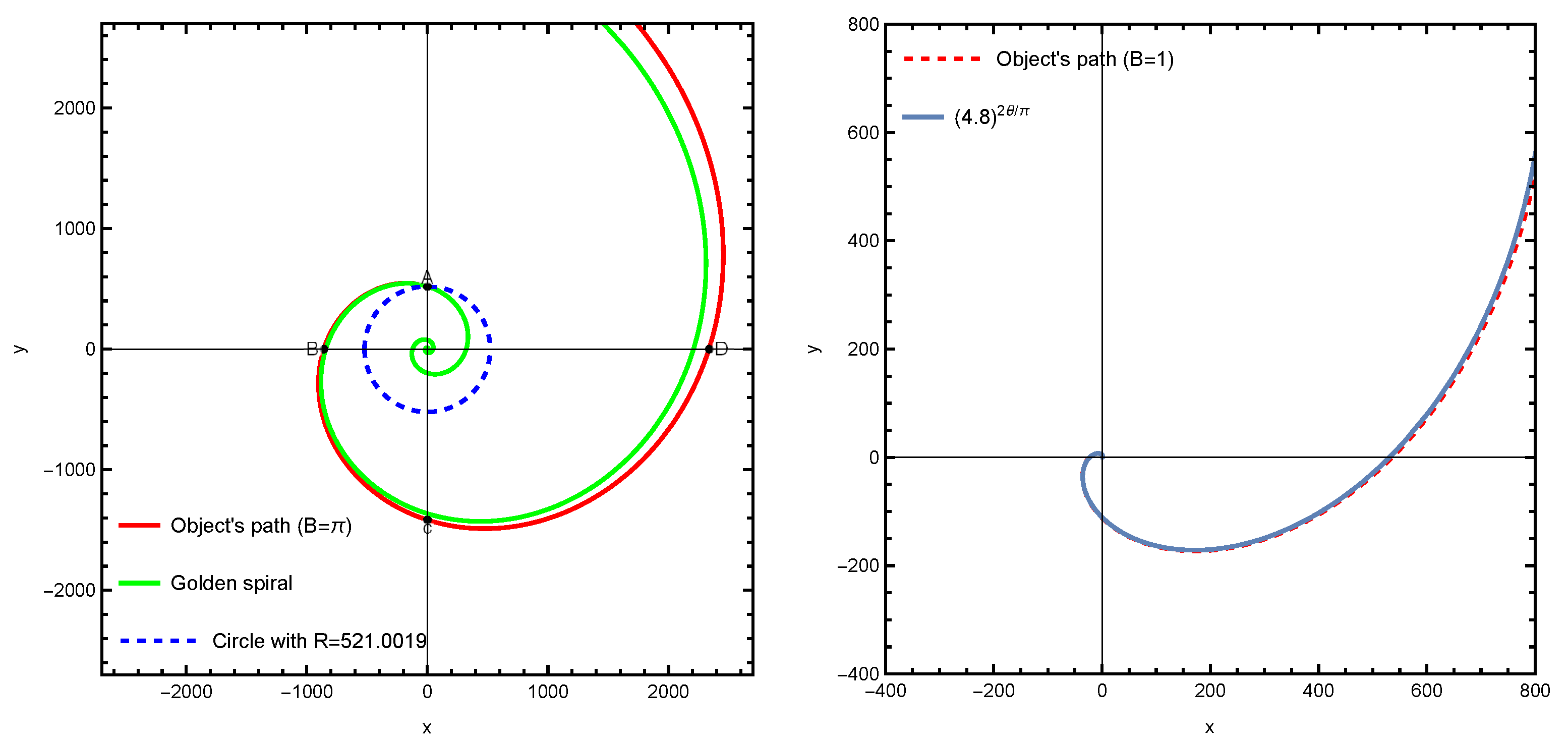
Figure 3.
Illustration of the time mechanism for the 3D space crust at the quantum scale and its comparison with Einstein’s light cone.
Figure 3.
Illustration of the time mechanism for the 3D space crust at the quantum scale and its comparison with Einstein’s light cone.
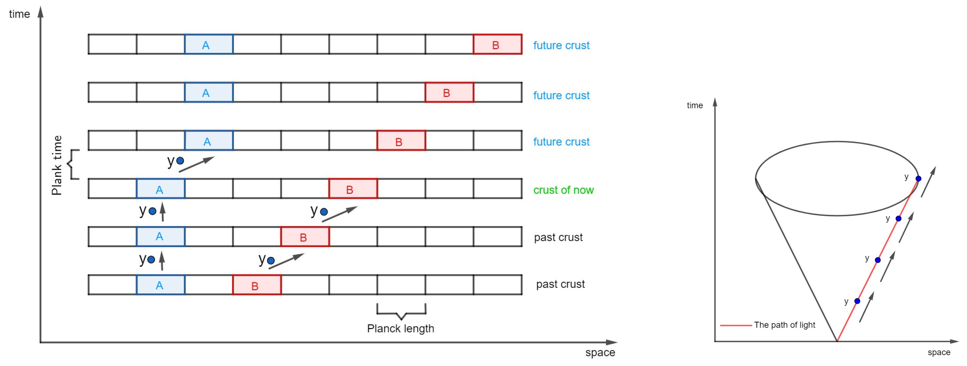
Figure 4.
The curvature of the light path from a distant galaxy within the four-dimensional sphere of the universe as it reaches Earth.
Figure 4.
The curvature of the light path from a distant galaxy within the four-dimensional sphere of the universe as it reaches Earth.
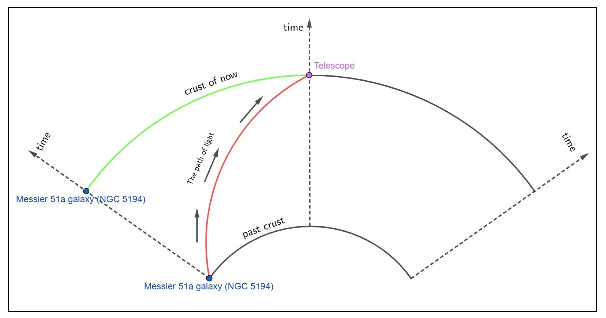
Figure 5.
The curvature of the space crust throughout the birth (R point) and death (P point) phases of a black hole within the four-dimensional sphere of the universe.
Figure 5.
The curvature of the space crust throughout the birth (R point) and death (P point) phases of a black hole within the four-dimensional sphere of the universe.
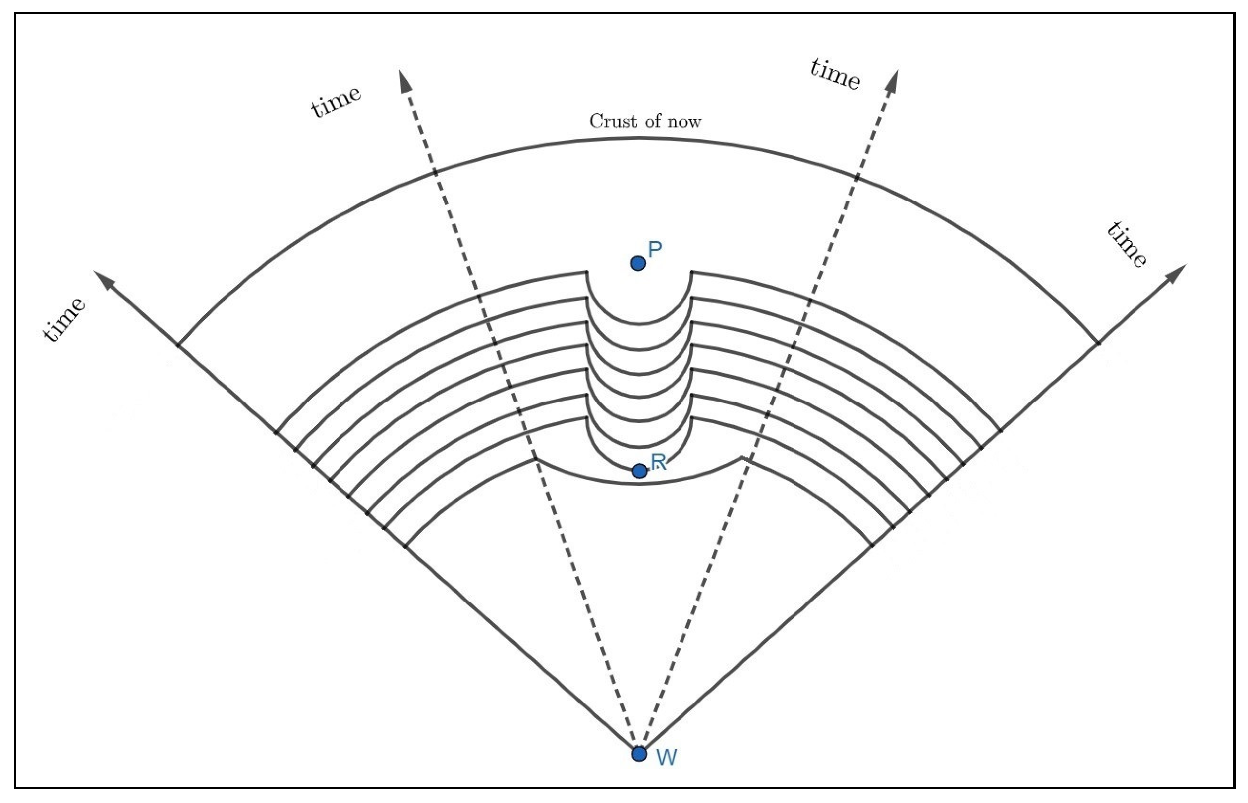
Figure 6.
The position of the first mirror point relative to Earth within the four-dimensional sphere of the universe.
Figure 6.
The position of the first mirror point relative to Earth within the four-dimensional sphere of the universe.
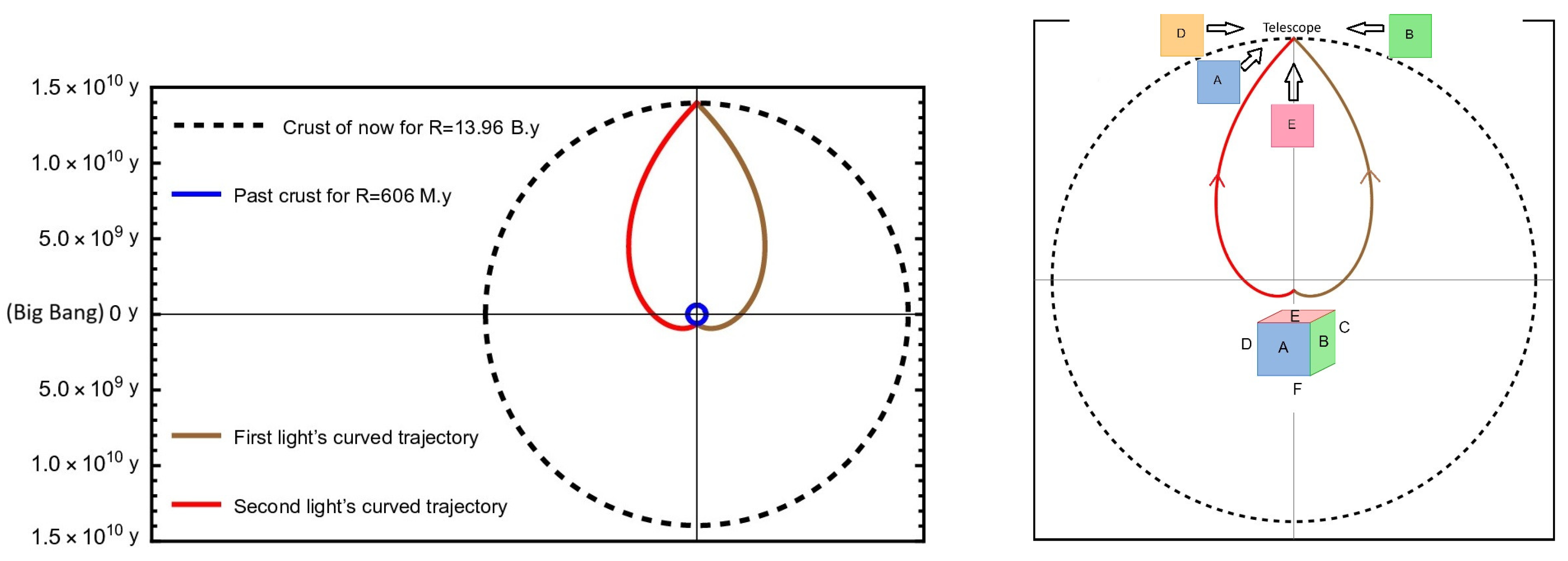
Figure 7.
The positions of four points, each with a phase difference of , during the final complete cycle of light reaching Earth within the four-dimensional sphere of the universe.
Figure 7.
The positions of four points, each with a phase difference of , during the final complete cycle of light reaching Earth within the four-dimensional sphere of the universe.
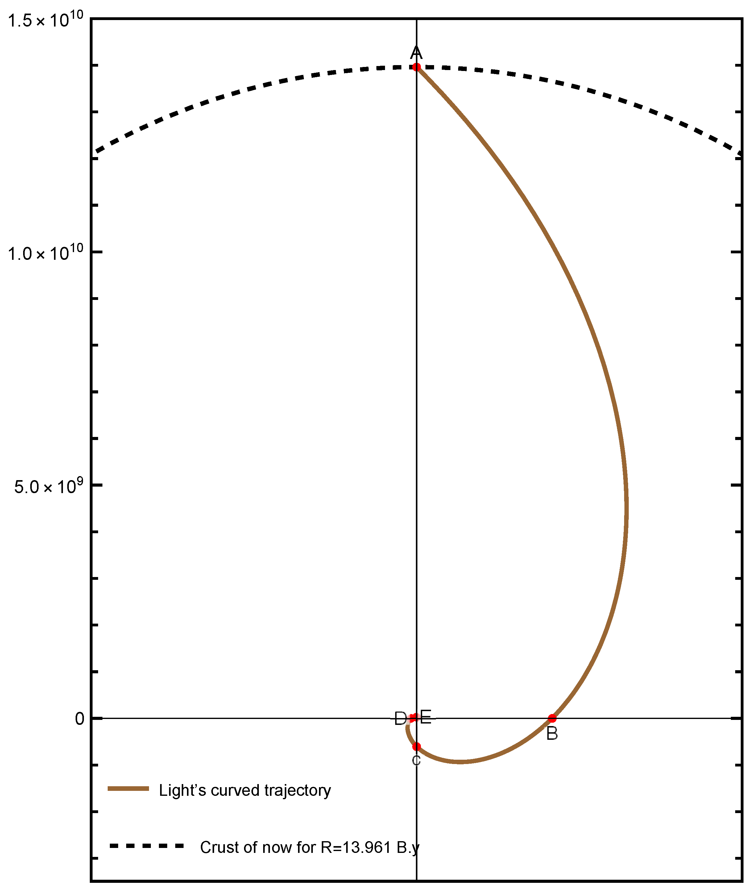
Figure 8.
Time-dependent distance between Earth and Messier 51a, depicted by colored arc segments.

| Points | ||
|---|---|---|
| A | 521 | 1.648 |
| B | 859 | 1.650 |
| C | 1418 | 1.643 |
| D | 2330 | - |
Table 2.
Benchmark properties for the mediator Y when modelled as a gauge-singlet scalar.
| Property | Value (SI) | Value (natural units) |
|---|---|---|
| Electric charge | 0 C | 0 (gauge singlet) |
| Spin | 0 | |
| Mass (benchmark) | ||
| Compton time | ||
| Effective temporal damping |
Table 3.
Variation of the Universe’s Radius Corresponding to Different Hubble Constant Values.
Table 4.
Various spatial distances of Messier 51a from Earth in light years.
| Path | Color | Spatial distance |
|---|---|---|
| Distance observed by telescope | brown | |
| Real distance at now | green | |
| Traveling distance | purple |
Table 5.
The time of mirror points after the Big Bang for results of in Table 3.
Table 5.
The time of mirror points after the Big Bang for results of in Table 3.
| 53382 | 49569 | ||
| 2008 | |||
Table 6.
The values of (), () and () for results of in Table 3.
Table 6.
The values of (), () and () for results of in Table 3.
Disclaimer/Publisher’s Note: The statements, opinions and data contained in all publications are solely those of the individual author(s) and contributor(s) and not of MDPI and/or the editor(s). MDPI and/or the editor(s) disclaim responsibility for any injury to people or property resulting from any ideas, methods, instructions or products referred to in the content. |
© 2026 by the authors. Licensee MDPI, Basel, Switzerland. This article is an open access article distributed under the terms and conditions of the Creative Commons Attribution (CC BY) license (http://creativecommons.org/licenses/by/4.0/).
Copyright: This open access article is published under a Creative Commons CC BY 4.0 license, which permit the free download, distribution, and reuse, provided that the author and preprint are cited in any reuse.


